A Self-Learning Based Preference Model for Portfolio Optimization

Abstract

An investment in a portfolio can not only guarantee returns but can also effectively control risk factors. Portfolio optimization is a multi-objective optimization problem. In order to better assist a decision maker to obtain his/her preferred investment solution, an interactive multi-criterion decision making system (MV-IMCDM) is designed for the Mean-Variance (MV) model of the portfolio optimization problem. Considering the flexibility requirement of a preference model that provides a guiding role in MV-IMCDM, a self-learning based preference model DT-PM (decision tree-preference model) is constructed. Compared with the present function based preference model, the DT-PM fully considers a decision maker’s bounded rationality. It does not require an assumption that the decision maker’s preference structure and preference change are known a priori and can be automatically generated and completely updated by learning from the decision maker’s preference feedback. Experimental results of a comparison show that, in the case that the decision maker’s preference structure and preference change are unknown a priori, the performances of guidance and fitness of the DT-PM are remarkably superior to function based preference models; in the case that the decision maker’s preference structure is known a priori, the performances of guidance and fitness of the DT-PM is approximated to the predefined function based model. It can be concluded that the DT-PM can agree with the preference ambiguity and the variability of a decision maker with bounded rationality and be applied more widely in a real decision system.

1. Introduction

In recent years, the rapid development of China’s economy has increasingly improved people’s quality of life. A growing number of people are unwilling to bear their idle funds that have been depreciated by inflation, and participate in investment for financial management. For a positive correlation between the economic returns and the possible risks, investors tend to invest their discretionary funds in more than one financial product so as to disperse potential risks. Correspondingly, a financial management problem with portfolios has appeared. Harry Markowitz, a prominent American economist and Nobel laureate, first proposed the mean variance (MV) model [1,2] based on quantitative research, which represents the modern portfolio theory [3]. The MV model, which uses the mean and variance of existing returns to quantitatively describe the returns and risks of portfolio, has since been widely applied in the financial sector. Meanwhile, a number of different portfolio optimization models have been proposed to manage specific situations in the financial market. Among them, some models are derived by creating additional or variational objectives based on the MV model, e.g., skewness [4], volatility in the portfolios [5], mean absolute deviation [6], minimax [7], and value at risk [8,9]; some by incorporating additional constraints into the MV model, e.g., boundaries [10], cardinality [11], and transaction costs [12], or by relaxing existing constraints, such as weight from non-negativity to negativity [13]; and some by being extended before their suitability in a dynamic market, such as a prediction-based portfolio optimization model that can predict each stock’s future return [14]. Since these portfolio optimization models are almost multi-objective and are very difficult to solve efficiently using mathematical programming and exact methods [15,16], further attention has been paid to the metaheuristic algorithms that have displayed high performance levels in solving multi-objective optimization problems in other fields. These algorithms include the niched Pareto genetic algorithm II (NPGA-II) [17], the strength Pareto evolutionary algorithm 2 (SPEA2) [18], the multi-objective evolutionary algorithm based on decomposition (MOEA/D) [19], particle swarm optimization (PSO) [20], an artificial bee colony (ABC) [21], a biased-randomized iterated local search algorithm [22], and so on.

However, the outcome of a metaheuristic algorithm used for a portfolio optimization model is a Pareto front, which comprises numerous non-dominated solutions. In reality, an investor will not be interested in only some of them in accordance with his/her preferences. Generally, because it is not possible for an investor to select the one solution from such numerous solutions that is in his/her best interest, an interactive multi-criteria decision making (IMCDM) method is required. An IMCDM is composed of three parts: a search engine, the preference information and a preference model [23]. The search engine is responsible for generating non-dominated solutions, and normally adopts evolutionary multi-objective algorithms (EMO) due to their excellence in parallel computation. Based on a set of non-dominated solutions, a decision maker (DM) articulates his/her preference information. For the preference information, a preference model is built and used to guide the EMO in searching for the next generation of solutions.

Nearly all of the aforementioned EMOs have been extended to be applied in different IMCDMs and have achieved outstanding performances; the readers are referred to [24,25,26,27,28] for detailed reviews.

There are two types of preference information presented in the literature, quantitative and qualitative. The quantitative preference information includes reference points [29,30,31] or goal point [32], weights [32,33], reference directions [34,35], preference regions [36,37], and so on. Quantitative preference information is highly efficient in helping the IMCDM to obtain a DM’s preferred solution, but it demands a DM with high cognitive capability, which is not feasible in most cases [38,39]. The qualitative preference information is, in reality, more suitable with respect to a DM with bounded rationality [40,41]. As can be found by comparing solutions in pairs locally, the pairwise comparison is much easier for a bounded rational DM to provide his/her preferences than the other forms of qualitative preference information such as extremum selection [42,43], which requires comparing all the solutions on a global scope, and thus has been adopted by many IMCDMs [38,39,44]. Under the assumption that a DM with bounded rationality participated in an IMCDM for portfolio optimization, we adopt the pairwise comparison as the form of preference information so that our approach could cover a broader range of applications from the aspect of a DM’s cognitive capability.

In general, current IMCDMs adopt the preference model in the form of a function. The preference model uses a utility function U(y, w) to represent a user’s potential comprehensive evaluation on the objective function vector y of the multi-objective optimization problem while the user’s preference feedback results are used to update the value of the parameter vector w. The early utility functions are the weighted sum of optimization objectives [45]. Further, two novel representative utility functions are developed by Deb et al. [44], Battiti and Passerini [38], and Mukhlisullina et al. [39]. These two utility functions are the quadratic polynomial function and generic function of optimization objectives, respectively (the generic function form is determined by the kernel function preselected at the beginning of the decision). In order to manage the possible changes of user preferences in the decision-making process, Branke et al. [46] adopted the variable additive function set, which can convert the form of the utility function from a linear function to a Choquet integral function according to the complexity of user preferences in the decision process. An adaptive preference model [47] is built using a dynamic feature analysis, which can be suitable for the user preference changes in the decision making process.

Although different forms of function-based preference models are presented in IMCDMs, they are not capable of modeling the complicated preferences of a DM with bounded rationality if his/her preference structure is not known a priori and if they change unpredictably. Appropriate function forms (including the two forms adopted in variable additive function set) for the function based preference models should be predefined at the beginning of the decision-making process. These function forms imply the rational hypothesis that a DM can clearly predict his/her potential preference structure. However, the flexibility of the preference model is greatly limited by the preselected function form. Therefore, it is difficult to adapt to various changes of user preferences in the decision-making process. The recently proposed adaptive preference model is very effective in modeling a DM’s various preference changes, however, it can be only applied in a scenario where the features incorporated into the model by dynamic analysis have an equivalent impact on the DM’s preference with the optimization of the objective functions. In general, the optimization functions because the objectives of an optimization model are in principle the primary impact factors of the DM’s preference, and more important than other features.

In order to solve the portfolio optimization problem, with the objective of mitigating the restrictions of the function based preference models, this paper designs an interactive decision-making method by focusing on the research regarding a flexible and robust preference model. Considering the user’s limited cognitive capability [41,48], i.e., his/her preference structure is unlikely to be known a priori, and his/her preference may change arbitrarily in the process of decision-making process, this paper proposes a self-learning-based preference model. This model does not require any rational assumptions on the DM’s preference structure and preference changes. It can be generated and completely updated automatically and by learning the user’s preference feedback, thus, it can accommodate to a bounded rational user’s preference ambiguity at the beginning of and during variability in the decision-making process. Furthermore, the objective functions are the sole primary impact factors of the DM’s preferences, which allows the preference model to be applied through a more reasonable and general method.

Even though the MV model cannot cover all the application scenarios in the financial market, considering that as the modern portfolio theory [3], it has had a major impact on academic research and the financial industry as a whole [49], most of the portfolio optimization models are variants or extensions of this model, and recent studies showed that it is a more robust bi-objective model than other well-known models [50], this paper employed the MV model as the portfolio optimization problem with the aim that the research benefits could be extended to various applications based on or derived from it. At the same time, since so many EMOs have been studied in the literature and have been incorporated into different IMCDMs, we will select one from among those with the most successful applications in our IMCDM to be used for portfolio optimization.

The remainder of the paper is organized as follows: in Section 2, the interactive multi-criterion decision making system for portfolio optimization (MV-IMCDM) is developed; Section 3 proposes the self-learning based preference model used in MV-IMCDM; Section 4 presents the experimental results and the conclusions are summarized in Section 5.

2. Multi-Criteria Decision Making System for Portfolio Optimization MV-IMCDM

2.1. MV Model

In Markowitz’s portfolio theory, the return of the portfolio is represented by the expected rate of return, and the risk is represented by a covariance between the rates of return. Usually, the increase of the return indicates the increase of the risk. Therefore, investors should consider both return and risk simultaneously when selecting a portfolio. Markowitz’s classical portfolio MV model [1,2] can be expressed as:

$$\max \hspace{1em}{f}_1={\displaystyle \sum _{i=1}^N{\omega }_i{\mu }_i}$$

(1)

$$\min \hspace{1em}{f}_2={\displaystyle \sum _{i=1}^N{\displaystyle \sum _{j=1}^N{\omega }_i{\omega }_j{\sigma }_{ij}}}$$

(2)

$$\mathrm{s}.\mathrm{t}.{\displaystyle \sum _{i=1}^N{\omega }_i}=1$$

(3)

$$0\le {\omega }_i\le 1,i=1,\dots ,N$$

(4)

where N is the number of assets available to investors in the market, ${\mu }_i$($i=1,\dots ,N$) represents the expected rate of return of the ith asset, ${\sigma }_{\mathrm{ij}}$($i=1,\dots ,N$; $j=1,\dots ,N$) represents the covariance between the ith asset and the jth asset, ${\omega }_i$ is the decision variable which represents the investment ratio on the ith asset in the whole portfolio. Equations (1) and (2) represent the maximum return and the minimum risk of the portfolio respectively. Equation (3) indicates that the sum of the investment ratio on each asset is 1, that is, that all the existing funds are used for investment. Equation (4) requires that the investment ratio of each asset is non-negative.

As a multi-objective optimization problem, the Markowitz portfolio problem involves two objectives: return and risk. Therefore, seeking an optimal solution provides a balance and compromise between the two objectives, in order to find an efficient frontier of portfolio in the objective space. If a portfolio is efficient, then in the objective space, it must be the portfolio with the highest expected return under the same risk or the portfolio with the lowest risk under the same expected return. This is the common preference rule of investors. For portfolio a and b, if one of the following two conditions is satisfied:

$$f_2(a)\le f_2(b)\wedge f_1(a)>f_1(b)$$

(5)

$$f_1(a)\ge f_1(b)\wedge f_2(a)<f_2(b)$$

(6)

Then, portfolio a is better than portfolio b.

2.2. MV-IMCDM

In practical investments, investors have different preferences for expected risk and return. The extremely risk-aversive investor will choose the relatively safe portfolio with low risk and low return. By contrast, the risk-preferred investor will choose the investment with high risk and high return. This is the individual preference rule of investors.

In order to realize the common preference rules of investors, the portfolio is selected from the solutions produced by each generation of evolutionary computation of the EMO algorithm according to Equation (5) or (6). To realize the individual preference rules of investors, it is necessary to obtain the preference information of investors. Therefore, the interaction between user and the EMO algorithm is implemented to obtain a user’s preference feedback, then a preference model is constructed according to user’s preference feedback. The solutions generated by the algorithm are selected again according to the user’s preference model. With respect to the MV model for portfolio optimization, this paper designs the interactive multiple criteria decision making process (MV-IMCDM), as shown in Figure 1.

The MV-IMCDM system is composed of the EMO, user preference feedback (PF) and the preference model (PM). The user interacts with the EMO whenever it evolves by a certain number of generation. At this point, if the user is satisfied with the current best solution (i.e., the one with the highest rank among a set of solutions ordered by PM), the system will terminate. Otherwise, the system provides a set of solutions generated by the algorithm to the user for obtaining PF, then the PM is updated according to user’s PF. During the initial operation of EMO, because the user’s PM has not been generated, the solutions computed at each generation can only be organized according to the common preference principle. Once the user’s PM is produced, the solutions created at each generation will be organized first by the common preference principle (i.e., the non-dominance) and then by the individual preference principle (i.e., the PM). The same set of solutions will be used to calculate the evaluation index Acc of PM according to the orders provided by the PM and user’s PF, respectively.

So far, many EMO algorithms have been proposed to deal with multi-objective optimization problems. Among them, the non-dominated sorting genetic algorithm II (NSGA-II) [51] and the multi-objective evolutionary algorithm based on decomposition (MOEA/D) [52] are the two most influential methods. Studies show that they are very competitive with respect to the performance measures of proximity and diversity, an MOEA/D is better for some multi-objective optimization problems [39,53] while NSGAII is more suitable for other multi-objective optimization problems [54]. But for portfolio optimization problems [55,56,57] that are derived from the MV model, the MOEA/D outperforms the NSGA-II for the two performance measures. These portfolio optimization problems have two objectives of return and risk and very similar constraints as the MV model., The portfolio optimization problem in [57] specifically considers transaction cost in three cases: zero, fixed and proportional. This problem in the case of zero transaction cost is equivalent to the MV model. Hence, the MOEA/D is selected as the EMO algorithm of MV-IMCDM system.

As previously indicated, the user’s PF is provided based on a pairwise comparison, which is used to direct the EMO in searching for a user’s preferred solution through PM. Therefore, PM plays a key guiding role in IMCDM. The construction of PM is crucial for an MV-IMCDM design. The specific design of PM is given in the following section.

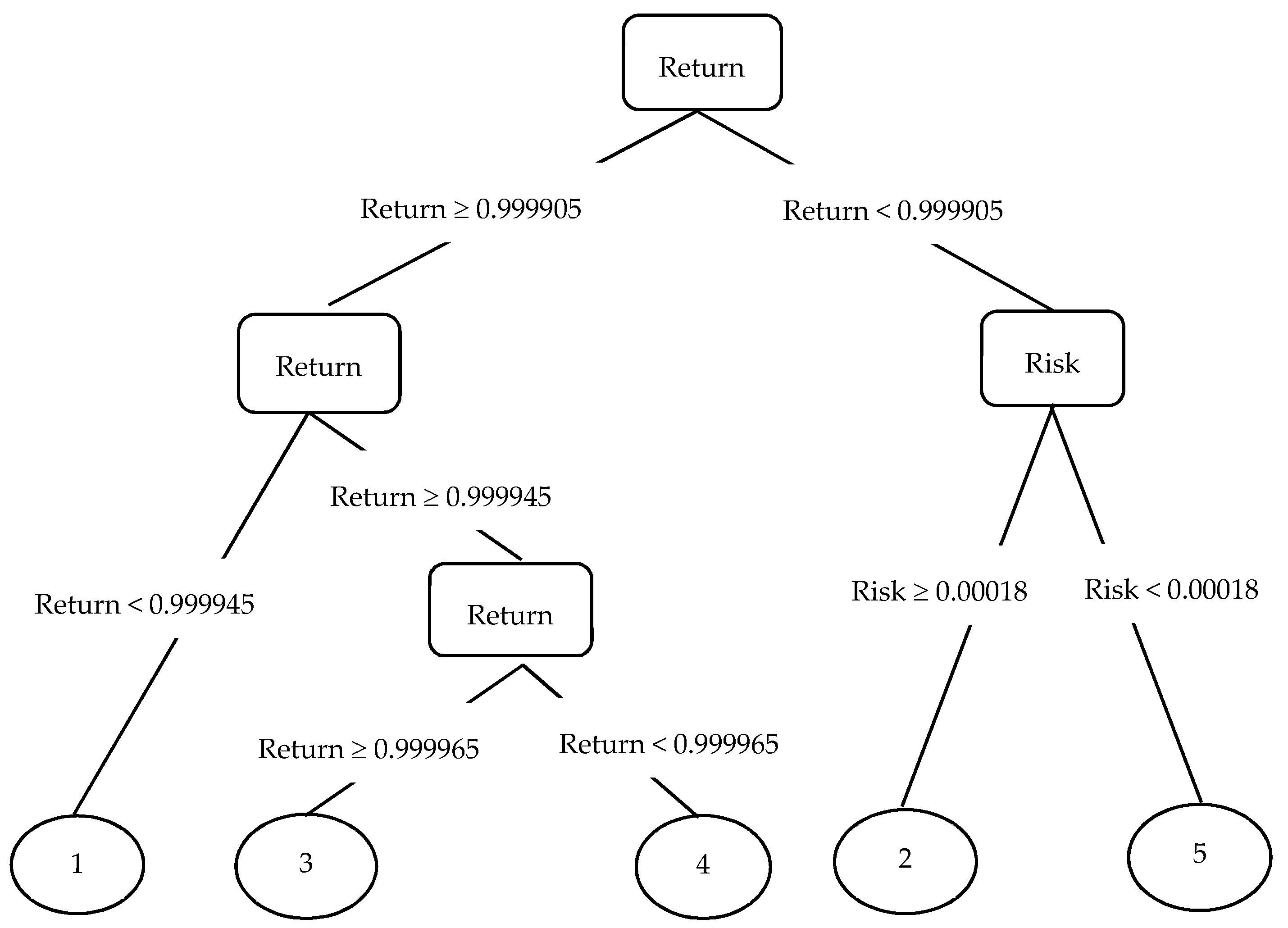
3. The Self-Learning Based Preference Model DT-PM

3.1. Construction of DT-PM

A PM is a formal description of user’s potential preferences. With the consideration of user’s bounded rationality, a PM with high flexibility can accommodate fora user’s ambiguous understanding of an optimization problem at the beginning of the decision-making process and any possible changes of a user’s preferences in the process of decision-making. Therefore, a flexible PM should have three basic characteristics:

(1) Free form:

The free form of PM can ensure the free change of the PF without limitations on any pre-defined preference structure so as to accommodate to the various potential changes of user preferences.

(2) Adaptive update:

The sole basis for building PM is the user’s PF for a set of solutions. If user’s preference changes, PM can only be updated according to user’s PF.

(3) Transparency of results:

The process of interaction between user and system is the process of improving user’s cognitive ability. A set of ordered solutions generated by the guidance of PM is an important experience for users to be able to gradually identify their potential preferences. Therefore, the PM needs to provide a transparent explanation of the produced ordered solutions.

Considering the three characteristics of a flexible PM in MV-IMCDM, this paper designs a PM based on self-learning, that is, by using the PM as a classifier. The classifier has a free form, and a set of ordered solutions obtained by the user’s PF can be used as a data set. Under a certain machine learning algorithm, the classifier is generated completely based on a data set to realize a self-adaptive update. The PM based on self-learning is shown in Figure 2.

There are many kinds of classifiers, such as neural network [58] and Bayes [59]. However, these classifiers cannot provide a transparent interpretation of the classified results. For some ensemble classifiers with remarkable performance [60], the classified results of their member classifiers are transparent. However, because the classified result is the aggregation of the member classifiers’ classification, ensemble classifiers cannot transparently explain the classified result.

Decision tree (DT) [61] is a sequence classifier, which consists of some simple logic tests. Each test compares an attribute with a real value, and each path from the root node to the leaf node represents a classification rule. Figure 3 shows a classification rule derived from a decision tree. For the MV model, each test compares an objective function (return or risk) with a real value of the solution, and each leaf node represents the class label (preference level) of the solution that conforms to a classification rule. Because the classification rule of a decision tree is similar to human reasoning processes, the classified result is straightforward to understand. It is helpful to further users’ understanding of the problem, to make users’ PF more confident, and to accelerate the convergence of the interactive decision-making process.

At present, numerous learning algorithms for creating a decision tree have been proposed [62,63], among which the CART algorithm has the advantages of simplicity, high efficiency and wide application [64]. Therefore, MV-IMCDM uses the CART learning algorithm to construct the decision tree-preference model DT-PM.

3.2. Sample Space of DT-PM

Before constructing the preference model, the sample space of the model needs to be established. The preference model is constructed according to the non-inferior solutions of different fronts generated in the algorithm evolution, and these solutions on different fronts have different distribution characteristics. Therefore, the solutions on different fronts need to be mapped to the same feature space, and the preference model is built on the samples in the space. Firstly, with regard to the MV model of the portfolio optimization problem, the return is transformed into the minimum non-negative objective (the risk objective remains unchanged):

$$\min \hspace{1em}{z}_1=1-f_1=1-{\displaystyle \sum _{i=1}^N{\omega }_i{\mu }_i}$$

(7)

$$\min z_2=f_2={\displaystyle \sum _{i=1}^N{\displaystyle \sum _{j=1}^N{\omega }_i{\omega }_j{\sigma }_{ij}}}$$

(8)

Thus, the different non-inferior solutions on the same frontier reflect the different compromises between the two objective function values of return z₁ and risk z₂, that is, the proportional relationship between z₁ and z₂. Later, the model samples z = (z₁, z₂) are defined by the proportional relationship between the objective function values of solutions z = (z₁, z₂):

$${\zeta }_j=\frac{z_j}{{\displaystyle {\sum }_j{z}_j}}$$

(9)

All samples in space $\Omega$ = $\left\{{\displaystyle {\sum }_j{\zeta }_j=1}\right\}$ follow the same characteristic distribution. In the MV model, Equation (9) establishes one-to-one mapping between different non-inferior solutions on the same front and characteristic space $\Omega$.

3.3. Guidance of DT-PM

The DT-PM, which is generated adaptively based on user’s PF, realizes the individual preference rules of investors by guiding the EMO algorithm. The guidance of DT-PM to EMO is applied in two places:

(1) Preparation for the generation of offspring individuals:

In the EMO algorithm, the offspring individuals are generated according to the parent individuals. In order to create the offspring individuals in accordance with user preferences, DT-PM is used to sort the parent individuals and select better parent individuals prepared for the recombination, to produce offspring individuals.

(2) Generation of offspring population:

Since there is no guarantee that all the offspring individuals generated each time are better than the parent individuals in the evolutionary process of EMO, in order to produce offspring population in accordance with user preferences, we need to merge the parent with the offspring individuals and sort them according to DT-PM, then select the better individuals to form the offspring population. Considering the common preference rules of investors, before using DT-PM to rank the merged individuals, we first rank them according to the criterion of non-dominance.

For an EMO algorithm, the selection of offspring population is generally based on two criteria, proximity (i.e., non-dominance) and diversity, while in our IMCDM, the selection of offspring population is based firstly on non-dominance and then on DT-PM; the preference model of DT-PM guides the EMO in our IMCDM to search for the DM’s preferred solution.

4. Experimental Evaluation

4.1. Experimental Design

The data used in the experiment are stock data of the A-share main board market in Shanghai and Shenzhen from 1 January to 31 December 2019 in RESSET [65,66]. Stocks in the same or similar industries may be affected by the same factors. For the selection of applied stock data to disperse risks, 2849 stocks in 18 different industries are randomly selected according to their categories. The expected return rate is expressed by the average monthly return rate of the selected stock calculated from 1 January to 31 December 2019.

Table A1. The 18 selected stocks and their returns.

Stock Category and Code	Company Stock Code	Company in Short	Expected Return
agriculture, forestry, husbandry, fishery (A)	002458	Yisheng Stock	0.146350
mining (B)	601899	Zijin Mining	0.035467
manufacturing (C)	600809	Shanxi Fenjiu	0.087283
electricity, heating, gas, water, supply (D)	601139	Shenzhen Gas	0.037375
architecture (E)	002140	Donghua Tech	0.038983
wholesale, retailer (F)	603708	Jiajiayue	0.041692
transportation, storage, post (G)	601111	Air China	0.026667
accommodation, catering (H)	000428	Huatian Hotel	0.007550
information (I)	600570	Hangseng Elec	0.063117
finance (J)	000001	Pingan Bank	0.052067
estate (K)	600383	Jingdi Group	0.043716
lease, business service (L)	601888	CITS	0.036816
science, technique (M)	002887	Huayang Intl	0.035520
irrigation, environment, infrastructure (N)	000069	Green Ecology	0.024300
education (P)	002607	Zhonggong Edu	0.043266
sanitation, society (Q)	300015	Aier Eye	0.059350
culture, PE, entertainment (R)	300251	Ray Media	0.043150
composite (S)	600455	Broadcom Shares	0.044383

in Appendix A shows the expected return rate of the selected stock.

The algorithm parameter settings for the MOEA/D in MV-IMCDM are inherited from [57], for which the portfolio optimization problem is the same as the MV model, except when considering the transaction cost for each asset. The MOEA/D performs better than NSGA-II not only in the case of zero transaction cost (in this case, the portfolio optimization problem is just the MV model) but also in the case of a non-zero transaction cost. These parameter settings are decided through the comparison of MOEA/D and NSGA-II for a broad range of multi-objective optimization problems included in the authors’ previous work [53], in which MOEA/D performs better than NSGA-II. The results have been referenced by the following works [67,68,69,70], which employed MOEA/D for many other multi-objective optimization problems and achieved superior performances. The algorithm parameters include population size s = 100, maximum generations max_t = 100, polynomial mutation probability $p_m$ = 1/N (N is the number of assets) and distribution index ${\eta }_m$, differential evolution crossover probability CR =1.0 and scaling factor F = 0.5, for details see [53,57]. The key parameters related to the interaction in MV-IMCDM are: maximum interaction number max_it = 20, interaction step size (the number of generations between two adjacent interactions) gen = 5 and number of solutions given to the DM for PF st = 5. These interaction parameter settings are borrowed from a pioneering and influential interactive approach, [44], which used pairwise comparison as the PF, which we also used for our MV-IMCDM.

In IMCDM, the user’s PF is simulated by a function [44,71]. As of yet, there is no common rule on the design of these simulation functions. The aim of this research is to investigate a flexible preference model that is suitable for a DM with bounded rationality, and the experimental design is to evaluate the capability of the DT-PM to capture a DM’s preference structure and preference change in any form. In order to compare with the function based preference model, a polynomial function and more complex functions will be used as an emulated DM in our MV-IMCDM. Since exponential and logarithmic functions are much more complicated in their structure than a polynomial function, and have a highly distinctive form from one other, they are used to simulate the user’s PF in addition to a polynomial function. Their parameter values are selected based on the tuning so that the return and risk have a similar impact on the DM’s preferences for portfolios. The three functions, ordered from the simplest to the most complex are as follows:

$$V(z_1,z_2)=10z_1^3+0.06z_2$$

(10)

$$V(z_1,z_2)=e^{3.1z_1}+2.64z_2$$

(11)

$$V(z_1,z_2)=-\ln (z_1)+15.625z_2$$

(12)

where $z_1$ and $z_2$ are the optimization objectives of MV model expressed in Equations (7) and (8), respectively. In order to verify the effectiveness of the DT-PM preference model in MV-IMCDM, we compare the effects of DT-PM with two representative function preference models: the linear function [45] and the general polynomial function [38,39,44]. The two function preference models are denoted as L-PM and G-PM respectively. The comparison is divided into two categories: where the user’s preference have not changed, and where changes have been made during the decision-making process. In the first case, the user’s PF is emulated by Equations (10), (11) and (12) respectively. In the second case, the user’s PF is simulated by Equations (10)–(12) successively at stages of the decision-making process.

The experimental results are evaluated by two indices. The first is the guidance index which is commonly used in IMCDM, and is measured by the distance Diff between the obtained solution by IMCDM and the user’s real preferred solution. As a DM’s preference is emulated by a function V(.), the solution on the Pareto front obtained by the EMO with the highest functional value represents a DM’s real preferred solution. Therefore, Diff is a measurement on the basis of the DM’s satisfaction with the solution produced by IMCDM. It is noted that there may be a number of solutions produced by IMCDM depending on the precision of a DM’s preference articulation. If multiple solutions are produced by IMCDM, then the representative one is selected for the computation of Diff. The second is the fitness index, which is measured by the accuracy Acc of the preference model DT-PM. For a set of non-dominated solutions, there are two class labels, one is predicted by the DT-PM which is built at a previous interaction based on the DM’s preference feedback; the other is given by the DM in terms of an emulated function V(.). The Acc is computed based on the comparison of these two class labels for the same set of non-dominated solutions. Since the predicted class label represents a DM’s preference at a previous interaction, the value of Acc can reflect a DM’s preference change between two adjacent interactions. If Acc has a lower value, it reflects a greater preference change of the DM between adjacent interactions. There are two potential reasons for this: one is that the DM is not satisfied with the produced solution under the guidance of his/her preceding preference information in the form of a preference model such as DT-PM. Throughout successive interactions, the DM can gradually correct his/her preferences until a high value of Acc is achieved. The other is that the preference model is not capable of modeling the DM’s preferences. For example, if the DM’s preference structure is quadratic polynomial, a linear preference model will not achieve a high value. So, for a situation where the same number of interactions occur, the value of Acc is a measurement of a preference model’s capability of capturing user preferences. In this paper, the indices of Diff and Acc are used for the evaluation of the proposed preference models.

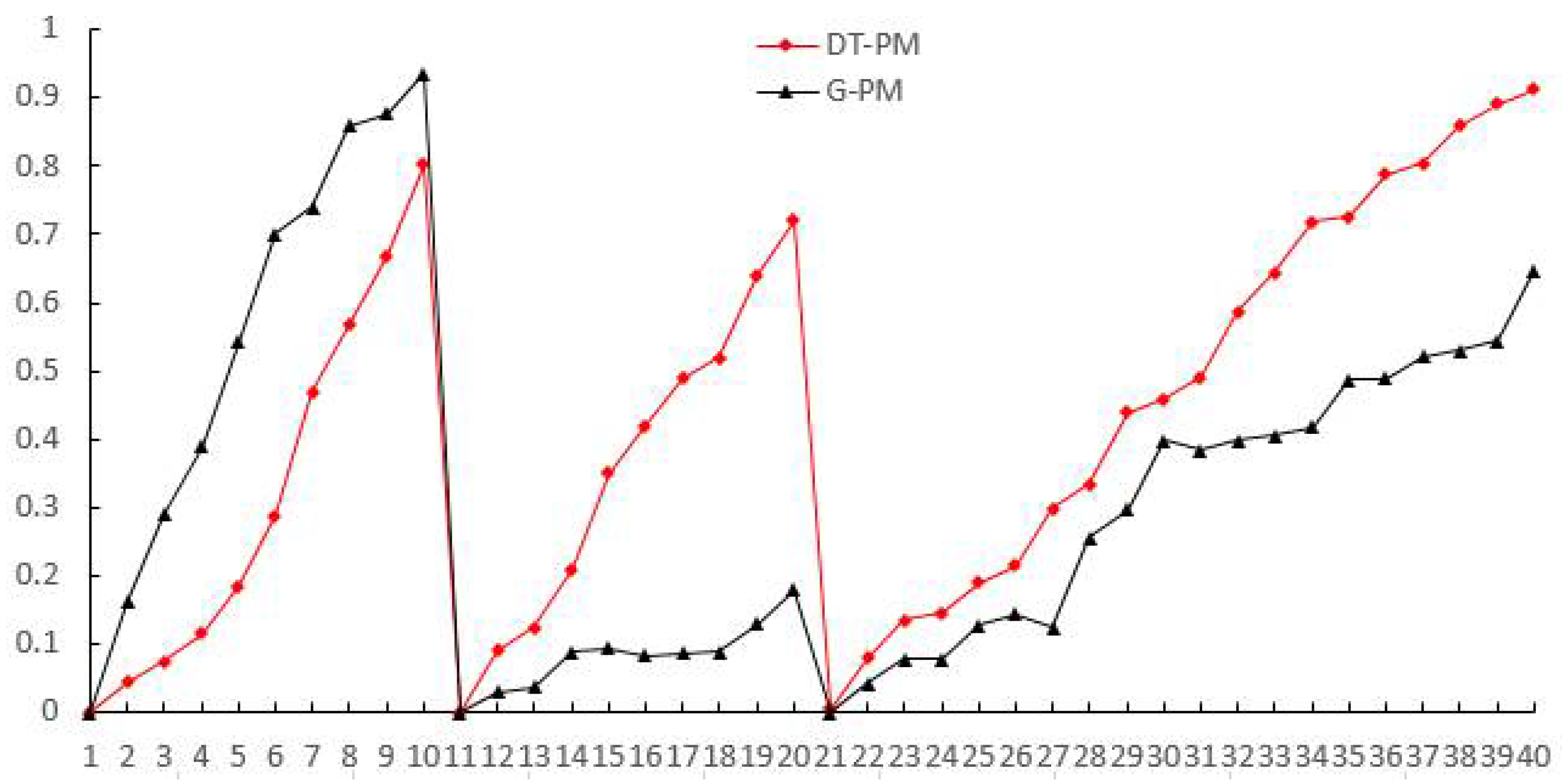
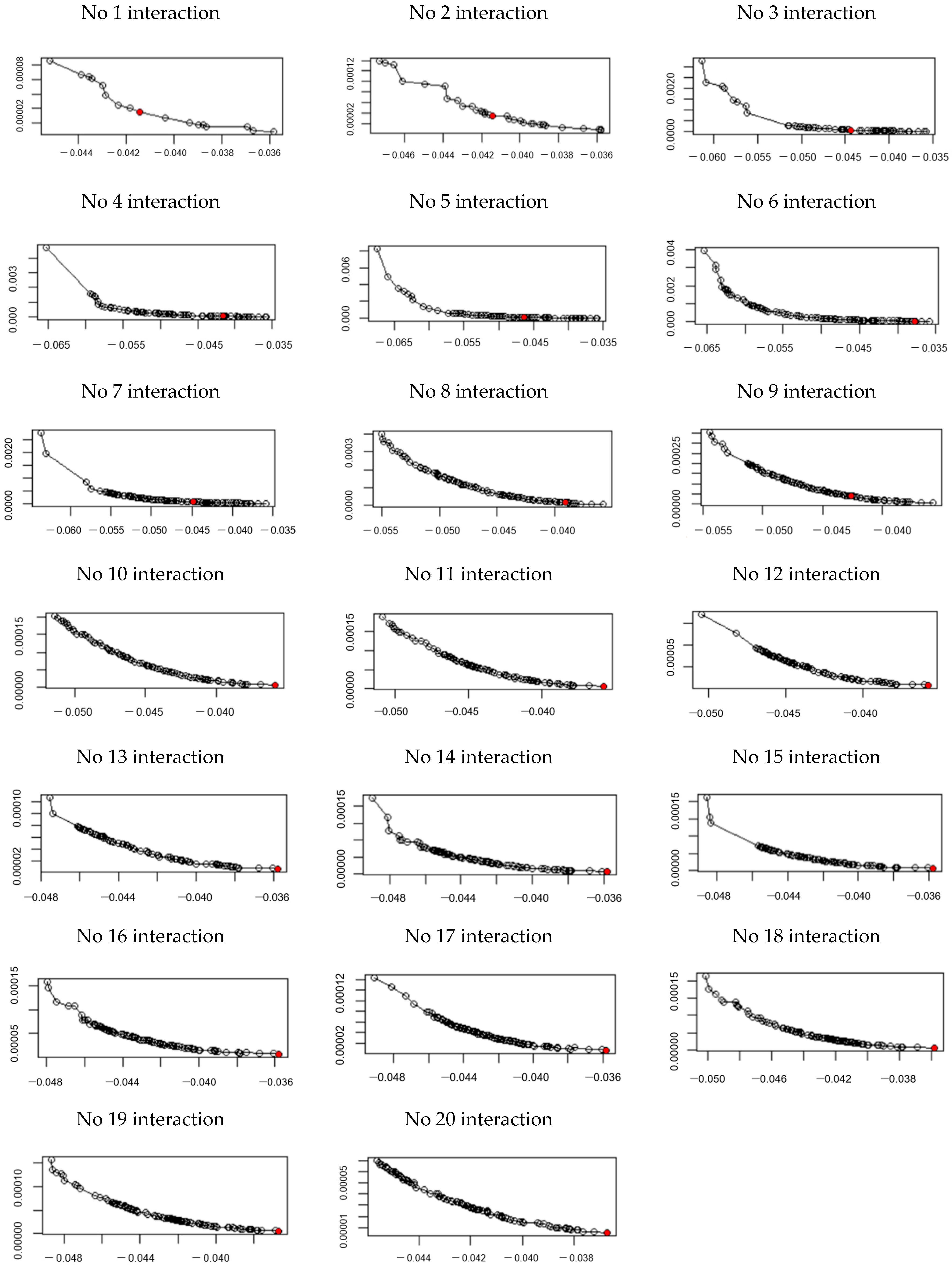
4.2. Experimental Results

The experimental results are presented in the following two cases.

(1) User’s preferences have no change:

Table 1. Comparative results based on user PF simulated by polynomial function (10).

PMs	Diff	Acc
DT-PM	28.537 × 10−9	0.913
L-PM	451.72 × 10−9	0.483
G-PM	2.054 × 10−9	0.979

,

Table 2. Comparative results based on user PF simulated by exponential function (11).

PMs	Diff	Acc
DT-PM	0.6042 × 10−9	0.929
L-PM	253.233 × 10−9	0.628
G-PM	5.726 × 10−9	0.822

and

Table 3. Comparative results based on user PF simulated by logarithmic function (12).

PMs	Diff	Acc
DT-PM	1.669 × 10−7	0.948
L-PM	236.043 × 10−7	0.554
G-PM	11.759 × 10−7	0.831

show the comparative results of three preference models based on user PF simulated by polynomial function (10), exponential function (11) and logarithmic function (12), respectively.

From Table 1, it can be seen that G-PM has the smallest Diff and the largest Acc, which indicates that the solution obtained by G-PM is closest to the user’s real preferred solution, and that G-PM has the greatest comprehensive ability to capture the user PF. This is because G-PM is a general polynomial function, which can easily adapt to the user PF simulated by polynomial function (10). The values of Diff and Acc of DT-PM are similar to those of G-PM, which indicates that DT-PM has a strong ability to adapt to polynomial functions. The values of Diff and Acc of L-PM are much worse than those of G-PM, which represents that if the preference model and the user’s preference structure are considerably different, it is difficult for the system to find a satisfactory solution.

If the user’s PF is a complex function, such as exponential function and a logarithmic function, Table 2 and Table 3 show that DT-PM provides a significant advantage over L-PM and G-PM.

(2) User’s preferences have changes:

In the interaction interval [1, 10], [11, 20] and [21, 40], the users’ preferences are simulated by polynomial function (10), exponential function (11) and logarithmic function (12) respectively.

Table 4. Comparative results under variable user preferences.

PMs	Diff	Acc
DT-PM	2.485 × 10−4	0.887
G-PM	3.722 × 10−4	0.573

shows the performance comparison of the preference models DT-PM and G-PM. It is evident that DT-PM is superior to G-PM in both Diff and Acc values.

In order to further investigate the adaptive capacity of the two preference models to the change of user preferences, we obtain their Acc values at each interaction in the decision-making process, as shown in Figure 4. In the interaction interval [1, 10], because the user’s PF is expressed by a polynomial function, G-PM shows better performance, which is consistent with the conclusion in Table 1. In the interaction intervals [11, 20] and [21, 40], DT-PM shows better performances because user’s PF is represented by a non-polynomial function (exponential function and logarithmic function), which confirms the conclusions in Table 2 and Table 3. It can also be seen from Figure 4 that when user preferences change (at the 11th and 21st interactions), the Acc values of both preference models almost drop to zero. This is because the user has a shifted preference structure simulated by an exponential function at the 11th interaction and a logarithmic function at the 21st interaction, respectively, which is fundamentally different from that simulated by a polynomial function at the 10th interaction and an exponential function at the 20th interaction, respectively. Both preference models, DT-PM and G-PM, are unable to accommodate for such a drastic preference change. It should be acknowledged that at the 1st interaction, the user’s PF is only used to initiate a preference model for which the Acc value is set to zero. Through the successive interactions, the Acc values of both preference models gradually increase. It is obvious that between two adjacent interactions, the Acc values of DT-PM recover to a higher level, which illustrates the impressive ability of DT-PM to capture a user’s arbitrary preference change.

The comparative experimental results have showed that the proposed DT-PM is highly appropriate for modeling a DM’s preference structure and preference change in any form. Under the guidance of DT-PM, the IMCDM will search for solutions in accordance with his/her preferences (via preference feedback). As a result, the frontier points are not distributed evenly but evolve into increasingly crowded clusters, the so called region of interests [72], from which the user preferred solution is determined by DT-PM. Figure A1 demonstrates the evolution of the frontier points and the user preferred solution under guidance of DT-PM in MV-IMCDM during interactions.

5. Conclusions

In this paper, in order to solve the portfolio optimization problem of the MV model, an interactive multi-criteria decision making system MV-IMCDM is designed to help users find a satisfactory portfolio. Considering the bounded rational user’s unpredictable preference structure and preference changes, a self-learning based preference model DT-PM is constructed. Compared with the commonly used functional preference model of a pairwise comparison based PF, the proposed DT-PM has several outstanding advantages: first of all, DT-PM does not require an assumption on a DM’s preference structure, it is entirely generated from a DM’s preference feedback; while for a functional preference model, a certain functional form should be predetermined a priori, which implicitly assumes that a DM’s preference structure is known and defined by the predetermined functional form. Secondly, the DT-PM is induced from a machine learning algorithm based on a DM’s feedback, and admits the DM to have a free change of his/her preferences; but since the functional form is predetermined for a functional preference model, a DM’s preference change is restricted to the range defined by the parameters in the function, which means that a DM’s preferences can have a minor change reflected by the parameter values of the function but cannot have a major change, which is reflected by the functional form. Next, the DT-PM can meet the demand of a DM with bounded rationality who uses an IMCDM, e.g., MV-IMCDM. Due to the DM’s limited background knowledge of the optimization problem such as MV, he/she may have a very vague preference at the beginning of the decision-making process, but through interactions, his/her understanding of the optimization problem may evolve in an unpredictable manner, and as a result, his/her vague preference may change in a free style. So the DT-PM is well- suited to the unpredictable evolution of a DM’s preferences in IMCDM. The functional preference model demands that the DM involved in an IMCDM to preselect a function form for his/her preferences a priori, and he/she should be much more rational in the understanding of the optimization problem as well as of his/her preferences than a DM with bounded rationality. Finally, the DT-PM can be used in a wider range of IMCDMs while it is also capable of modeling for a rational DM; but the functional preference model can only be used in an IMCDM, in which a rational DM is involved. The experimental results show that in the case of unpredictable user preferences, the guidance and appropriateness provided by a DT-PM are significantly better than in the functional preference model. Even when the preference structure is known a priori, the guidance and fitness of DT-PM can approximate the preset functional model.

Even though the DT-PM has demonstrated promising performances in MV-IMCDM, there are still investigations to be conducted while it is used to solve the challenging issues that have emerged in IMCDM with a complicated application background. In the present IMCDMs, a DM interacts with the algorithm after a certain number of generations of evolutionary computation. This interaction mechanism permits a DM to change his/her preferences at a given time during the decision-making process, which does not satisfy requirements if a DM would like to change preferences at his/her convenience. For this purpose, a more flexible interaction mechanism is to be investigated by the utilization of the DT-PM. In some IMCDMs, a group of DMs are involved in the interaction so as to avoid potentially biased preferences that may emerge in the case of only one DM. Configuring a way in which the DT-PM can be used to model a group of DM’s preferences in consensus is a very challenging problem. In view of the variants of the MV model, incorporating additional constraints, e.g., short-selling [73,74], borrowing [75,76], et al., or considering portfolios of short positions [77], exchange-traded funds (ETFs) for multi-asset-class investing [78], et al., will make the portfolio optimization model more suitable for specific application scenarios, as there is an urgent need for the DT-PM to be extended for modeling a DM’s complicated preferences in interactive approaches. In addition, while the number of non-dominated solutions of a multi-objective optimization problem such as the MV model produced at each interaction is very large, the pruning method [79] is a very effective way of generating a set with a greatly reduced number of representative non-dominated solutions; the integration of the pruning method into our MV-IMCDM is a promising research topic that presents the potential of enhancing the system’s performances.

References

1. Markowitz, H. Portfolio selection. J. Financ. 1952, 7, 77–91. [Google Scholar]
2. Markowitz, H. Portfolio Selection: Efficient Diversification of Investments; Yale University Press: New York, NY, USA, 1959. [Google Scholar]
3. Xu, N.; Yuan, C. Research on credit business operation efficiency of commercial banks based on portfolio theory. Syst. Eng. Theory Prac. 2019, 39, 1643–1650. [Google Scholar]
4. Li, X.; Qin, Z.; Kar, S. Mean-variance-skewness model for portfolio selection with fuzzy returns. Eur. J. Oper. Res. 2010, 202, 239–247. [Google Scholar] [CrossRef]
5. Ehrgott, M.; Klamroth, K.; Schwehm, C.J. An MCDM approach to portfolio optimization. Eur. J. Oper. Res. 2004, 155, 752–770. [Google Scholar] [CrossRef]
6. Konno, H.; Yamazaki, H. Mean-absolute deviation portfolio optimization model and its applications to Tokyo stock market. Manag. Sci. 1991, 37, 519–531. [Google Scholar] [CrossRef] [Green Version]
7. Young, M.R. A minimax portfolio selection rule with linear programming solution. Manag. Sci. 1998, 44, 673–683. [Google Scholar] [CrossRef] [Green Version]
8. Jorion, P. Value at Risk: A New Benchmark for Measuring Derivatives Risk; Irwin Professional Publishers: New York, NY, USA, 1996; pp. 1–624. [Google Scholar]
9. Cui, X.; Sun, X.; Zhu, S.; Jiang, R.; Li, D. Portfolio optimization with nonparametric value at risk: A block coordinate descent method. Inf. J. Comput. 2018, 30, 454–471. [Google Scholar] [CrossRef]
10. Speranza, M.G. A heuristic algorithm for a portfolio optimization model applied to the Milan stock market. Comput. Oper. Res. 1996, 23, 433–441. [Google Scholar] [CrossRef]
11. Hardoroudi, N.D.; Keshvari, A.; Kallio, M.; Korhonen, P.J. Solving cardinality constrained mean-variance portfolio problems via MILP. Ann. Oper. Res. 2017, 254, 47–59. [Google Scholar] [CrossRef]
12. Paiva, F.D.; Cardoso, R.T.N.; Hanaoka, G.P.; Duarte, W.M. Decision-making for financial trading: A fusion approach of machine learning and portfolio selection. Expert Sust. Appl. 2019, 115, 635–655. [Google Scholar] [CrossRef]
13. Kim, J.H.; Kim, W.C.; Fabozzi, F.J. Portfolio selection with conservative short-selling. Financ. Res. Lett. 2016, 18, 363–369. [Google Scholar] [CrossRef]
14. Ma, Y.; Han, R.; Wang, W. Prediction-based portfolio optimization models using deep neural networks. IEEE Access 2020, 8, 115393–115405. [Google Scholar] [CrossRef]
15. Ertenlice, O.; Kalayci, C.B. A survey of swarm intelligence for portfolio optimization: Algorithms and applications. Swarm Evol. Comput. 2018, 39, 36–52. [Google Scholar] [CrossRef]
16. Altinoz, M.; Altinoz, O.T. Systematic initialization approaches for portfolio optimization problems. IEEE Access 2019, 7, 57779–57794. [Google Scholar] [CrossRef]
17. Anagnostopoulos, K.P.; Mamanis, G. The mean-variance cardinality constrained portfolio optimization problem: An experimental evaluation of five multiobjective evolutionary algorithms. Expert Syst. Appl. 2011, 38, 14208–14217. [Google Scholar] [CrossRef]
18. García-Rodríguez, S.; Quintana, D.; Galván, I.M.; Viñuela, P.I. Portfolio optimization using SPEA2 with resampling. In Proceedings of the Intelligent Data Engineering and Automated Learning (IDEAL 2011), Norwich, UK, 7–9 September 2011; pp. 127–134. [Google Scholar]
19. He, Y.; Aranha, C. Solving portfolio optimization problems using MOEA/D and levy flight. Adv. Data Sci. Adapt. Anal. 2020, 12, 1–34. [Google Scholar]
20. Chen, C.; Zhou, Y. Robust multiobjective portfolio with higher moments. Expert Syst. Appl. 2018, 100, 165–181. [Google Scholar] [CrossRef]
21. Gao, W.; Sheng, H.; Wang, J.; Wang, S. Artificial bee colony algorithm based on novel mechanism for fuzzy portfolio selection. IEEE Trans. Fuzzy. Syst. 2019, 27, 966–978. [Google Scholar] [CrossRef]
22. Kizys, R.; Juan, A.A.; Sawik, B.; Calvet, L. A biased-randomized iterated local search algorithm for rich portfolio optimization. Appl. Sci. 2019, 9, 3509. [Google Scholar] [CrossRef] [Green Version]
23. Xin, B.; Chen, L.; Chen, J.; Ishibuchi, H.; Hirota, K.; Liu, B. Interactive multiobjective optimization: A review of the state-of-the-art. IEEE Access 2018, 6, 41256–41279. [Google Scholar] [CrossRef]
24. Branke, J.; Branke, J.; Deb, K.; Miettinen, K.; Slowiński, R. Multiobjective Optimization: Interactive and Evolutionary Approaches; Springer-Verlag: West Berlin, Germany, 2008; pp. 1–470. [Google Scholar]
25. Köksalan, M.; Wallenius, J.; Zionts, S. An early history of multiple criteria decision making. J. Multi-Criteria Decis. Anal. 2016, 20, 87–94. [Google Scholar] [CrossRef]
26. Meignan, D.; Knust, S.; Frayret, J.-M.; Pesant, G.; Gaud, N. A review and taxonomy of interactive optimization methods in operations research. ACM Trans. Interact. Intell. Syst. 2015, 5, 1–43. [Google Scholar] [CrossRef]
27. Allmendinger, R.W.; Ehrgott, M.; Gandibleux, X.; Geiger, M.J.; Klamroth, K.; Luque, M. Navigation in multiobjective optimization methods. J. Multi-Criteria Decis. Anal. 2017, 24, 57–70. [Google Scholar] [CrossRef]
28. Huber, S.; Geiger, M.J.; de Almeida, A.T. Multiple Criteria Decision Making and Aiding; Springer: West Berlin, Germany, 2019; pp. 1–309. [Google Scholar]
29. Deb, K.; Sundar, J. Reference point based multi-objective optimization using evolutionary algorithms. In Proceedings of the 8th Annual Conference on Genetic and Evolutionary Computation, Seattle, WA, USA; 2006; pp. 635–642. [Google Scholar]
30. Ruiz, A.B.; Saborido, R.; Bermúdez, J.D.; Luque, M.; Vercher, E. Preference-based evolutionary multi-objective optimization for portfolio selection: A new credibilistic model under investor preferences. J. Glob. Optim. 2020, 76, 295–315. [Google Scholar] [CrossRef]
31. Zhou-Kangas, Y.; Miettinen, K. Decision making in multiobjective optimization problems under uncertainty: Balancing between robustness and quality. OR Spectr. 2019, 41, 391–413. [Google Scholar] [CrossRef] [Green Version]
32. Hafiz, F.; Swain, A.; Mendes, E. Multi-objective evolutionary framework for non-linear system identification: A comprehensive investigation. Neurocomputing 2020, 386, 257–280. [Google Scholar] [CrossRef] [Green Version]
33. Ruiz, F.; Luque, M.; Cabello, J.M. A classification of the weighting schemes in reference point procedures for multiobjective programming. J. Oper. Res. Soc. 2009, 60, 544–553. [Google Scholar] [CrossRef]
34. Deb, K.; Kumar, A. Interactive evolutionary multi-objective optimization and decision-making using reference direction method. In Proceedings of the 9th Annual Conference on Genetic and Evolutionary Computation, London, UK, 7–11 July 2007; pp. 781–788. [Google Scholar]
35. Li, X.; He, Q.; Li, Y.; Zhu, Z. Multi-areas outstanding covering optimization method of HF network based on preference ranking elimination NSGAII algorithm. J. Electron. Inf. Technol. 2017, 8, 1779–1787. [Google Scholar]
36. Liu, R.; Wang, R.; Feng, W.; Huang, J.; Jiao, L. Interactive reference region based multi-objective evolutionary algorithm through decomposition. IEEE Access 2016, 4, 7331–7346. [Google Scholar] [CrossRef]
37. Hu, J.; Yu, G.; Zheng, J.; Zou, J. A preference-based multi-objective evolutionary algorithm using preference selection radius. Soft. Comput. 2017, 21, 5025–5051. [Google Scholar] [CrossRef]
38. Battiti, R.; Passerini, A. Brain computer evolutionary multiobjective optimization: A genetic algorithm adapting to the decision maker. IEEE Trans. Evol. Comput. 2010, 14, 671–687. [Google Scholar] [CrossRef]
39. Mukhlisullina, D.; Passerini, A.; Battiti, R. Learning to diversify in complex interactive multiobjective optimization. In Proceedings of the 10th Metaheuristics International Conference (MIC 2013), Singapore, 5–8 August 2013; pp. 230–239. [Google Scholar]
40. March, J.G. Bounded rationality, ambiguity, and the engineering of choice. Bell J. Econ. 1978, 9, 587–608. [Google Scholar] [CrossRef]
41. Larichev, O.I. Cognitive validity in design of decision-aiding techniques. J. Multi-Criteria Decis. Anal. 1992, 1, 127–138. [Google Scholar] [CrossRef]
42. Fowler, J.W.; Gel, E.S.; Köksalan, M.; Korhonen, P.J.; Marquis, J.L.; Wallenius, J. Interactive evolutionary multi-objective optimization for quasi-concave preference functions. Eur. J. Oper Res. 2010, 206, 417–425. [Google Scholar] [CrossRef]
43. Köksalan, M.; Karahan, I. An interactive territory defining evolutionary algorithm: iTDEA. IEEE Trans. Evol. Comput. 2010, 14, 702–722. [Google Scholar] [CrossRef]
44. Deb, K.; Sinha, A.; Korhonen, P.J.; Wallenius, J. An interactive evolutionary multiobjective optimization method based on progressively approximated value functions. IEEE Trans. Evol. Comput. 2010, 14, 723–739. [Google Scholar] [CrossRef] [Green Version]
45. Pascoletti, A.; Serafini, P. Scalarizing vector optimization problems. J. Optim. Theory Appl. 1984, 42, 499–524. [Google Scholar] [CrossRef]
46. Branke, J.; Corrente, S.; Greco, S.; Słowiński, R.; Zielniewicz, P. Using Choquet integral as preference model in interactive evolutionary multiobjective optimization. Eur. J. Oper. Res. 2016, 250, 884–901. [Google Scholar] [CrossRef] [Green Version]
47. Hu, S.; Li, F.; Liu, Y.; Wang, S. A self-adaptive preference model based on dynamic feature analysis for interactive portfolio optimization. Int. J. Mach. Learn. Cybern. 2020, 11, 1253–1266. [Google Scholar] [CrossRef]
48. Rubinstein, A.; Ni, X. Modeling Bounded Rationality; China Renmin University Press: Beijing, China, 2005; pp. 1–220. [Google Scholar]
49. Kolm, P.N.; Tütüncü, R.; Fabozzi, F.J. 60 Years of portfolio optimization: Practical challenges and current trends. Eur. J. Oper. Res. 2014, 234, 356–371. [Google Scholar] [CrossRef]
50. Pavlou, A.; Doumpos, M.; Zopounidis, C. The robustness of portfolio efficient frontiers: A comparative analysis of bi-objective and multi-objective approaches. Manag. Decis. 2018, 57, 300–313. [Google Scholar] [CrossRef]
51. Deb, K.; Pratap, A.; Agarwal, S.; Meyarivan, T. A fast and elitist multiobjective genetic algorithm: NSGA-II. IEEE Trans. Evol. Comput. 2002, 6, 182–197. [Google Scholar] [CrossRef] [Green Version]
52. Zhang, Q.; Li, H. MOEA/D: A multiobjective evolutionary algorithm based on decomposition. IEEE Trans. Evol. Comput. 2007, 11, 712–731. [Google Scholar] [CrossRef]
53. Li, H.; Zhang, Q. Multiobjective optimization problems with complicated pareto sets, MOEA/D and NSGA-II. IEEE Trans. Evol. Comput. 2009, 13, 284–302. [Google Scholar] [CrossRef]
54. Cuate, O.; Schütze, O.; Grasso, F.; Tlelo-Cuautle, E. Sizing CMOS operational transconductance amplifiers applying NSGA-II and MOEAD. In Proceedings of the 2019 42nd International Convention on Information and Communication Technology, Electronics and Microelectronics (MIPRO), Opatija, Croatia, 20–24 May 2019; pp. 149–152. [Google Scholar]
55. Mishra, S.K.; Panda, G.; Majhi, R. A comparative performance assessment of a set of multiobjective algorithms for constrained portfolio assets selection. Swarm Evol. Comput. 2014, 16, 38–51. [Google Scholar] [CrossRef]
56. Rajabi, M.; Khaloozadeh, H. Investigation and comparison of the performance of multi-objective evolutionary algorithms based on decomposition and dominance in portfolio optimization. In Proceedings of the 2018 International Conference on Electrical Engineering (ICEE), Mashhad, Iran, 8–10 May 2018; pp. 923–929. [Google Scholar]
57. Zhang, Q.; Li, H.; Maringer, D.G.; Tsang, E.P.K. MOEA/D with NBI-style Tchebycheff approach for portfolio management. In Proceedings of the IEEE Congress on Evolutionary Computation, Barcelona, Spain, 18–23 July 2010; pp. 1–8. [Google Scholar]
58. Zhu, H.; Pei, L.; Jiao, L.; Yang, S.; Hou, B. Review of parallel deep neural network. Chin. J. Comput. 2018, 41, 1861–1881. [Google Scholar]
59. Zhu, J.; Hu, W. Recent advances in bayesian machine learning. J. Comput. Res. Dev. 2015, 52, 16–26. [Google Scholar]
60. Wang, J.; Yang, L.; Yang, M. Multitier ensemble classifiers for malicious network traffic detection. J. Commun. 2018, 39, 155–165. [Google Scholar]
61. Grąbczewski, K. Meta-Learning in Decision Tree Induction; Springer: New York, NY, USA, 2014; pp. 1–343. [Google Scholar]
62. Safavian, S.R.; Landgrebe, D. A survey of decision tree classifier methodology. IEEE Trans. Syst. Man Cybern. 1991, 21, 660–674. [Google Scholar] [CrossRef] [Green Version]
63. Bramer, M. Principles of Data Mining/Edition 4; Springer-Verlag: London, UK, 2020; pp. 1–571. [Google Scholar]
64. Loh, W.Y. Fifty years of classification and regression trees. Int. Stat. Rev. 2014, 82, 329–348. [Google Scholar] [CrossRef] [Green Version]
65. Zhu, S.; Yan, Y. Financial Data; Tsinghua University Press: Beijing, China, 2007. [Google Scholar]
66. Resset Financial Research Database. Beijing Juyuan Resset Data Technology Co., Ltd. ed. DB/OL. Available online: http://www.resset.cn/ (accessed on 26 May 2021).
67. Pal, S.; Qu, B.; Das, S.; Suganthan, P.N. Linear antenna array synthesis with constrained multi-objective differential evolution. Prog. Electromagn. Res. 2010, 21, 87–111. [Google Scholar]
68. Basak, A.; Pal, S.; Pandi, V.R.; Panigrahi, B.K.; Mallick, M.K.; Mohapatra, A. A novel multi-objective formulation for hydrothermal power scheduling based on reservoir end volume relaxation. In Proceedings of the 2010 International Conference on Swarm, Evolutionary, and Memetic Computing, Hyderabad, India, 18–19 December 2010; pp. 718–726. [Google Scholar]
69. Li, Y.; Zhou, A.; Zhang, G. An MOEA/D with multiple differential evolution mutation operators. In Proceedings of the 2014 IEEE Congress on Evolutionary Computation (CEC), Beijing, China, 6–11 July 2014; pp. 397–404. [Google Scholar]
70. Zhou, A.; Zhang, Q.; Zhang, G. A multiobjective evolutionary algorithm based on decomposition and probability model. In Proceedings of the 2012 IEEE Congress on Evolutionary Computation, Brisbane, Australia, 10–15 June 2012; pp. 1–8. [Google Scholar]
71. Ozbey, O.; Karwan, M.H. An interactive approach for multicriteria decision making using a Tchebycheff utility function approximation. J. Multi-Criteria Decis. Anal. 2014, 21, 153–172. [Google Scholar] [CrossRef]
72. Chen, L.; Xin, B.; Chen, J.; Li, J. A virtual-decision-maker library considering personalities and dynamically changing preference structures for interactive multi-objective optimization. In Proceedings of the 2017 IEEE Congress on Evolutionary Computation (CEC), Donostia, Spain, 5–8 June 2017; pp. 636–641. [Google Scholar]
73. Jiang, Y.C.; Cheam, X.J.; Chen, C.Y.; Kuo, S.Y.; Chou, Y.H. A novel portfolio optimization with short selling using GNQTS and trend ratio. In Proceedings of the 2018 IEEE International Conference on Systems, Man, and Cybernetics (SMC), Miyazaki, Japan, 7–10 October 2018; pp. 1564–1569. [Google Scholar]
74. Teplá, L. Optimal portfolio policies with borrowing and shortsale constraints. J. Econ. Dyn. Control 2000, 24, 1623–1639. [Google Scholar] [CrossRef]
75. Fu, C.; Lari-Lavassani, A.; Li, X. Dynamic mean-variance portfolio selection with borrowing constraint. Eur. J. Oper. Res. 2010, 200, 312–319. [Google Scholar] [CrossRef]
76. Deng, X.; Li, R. A portfolio selection model with borrowing constraint based on possibility theory. Appl. Soft Comput. 2012, 12, 754–758. [Google Scholar] [CrossRef]
77. Gibbons, M.R.; Ross, S.A.; Shanken, J. A test of efficiency of a given portfolio. Econometrica 1989, 57, 1121–1152. [Google Scholar]
78. Agrrawal, P. Using index ETFs for multi-asset class investing: Shifting the efficient frontier up. J. Index Invest. 2013, 4, 83–94. [Google Scholar]
79. Petchrompo, S.; Wannakrairot, A.; Parlikad, A.K. Pruning pareto optimal solutions for multi-objective portfolio asset management. Eur. J. Oper. Res. 2021. [Google Scholar] [CrossRef]
Figure 1. Interactive multiple criteria decision making process for MV model.
Mathematics 09 02621 g001
Figure 2. Self-learning based PM.
Mathematics 09 02621 g002
Figure 3. Classification rules derived from decision tree.
Mathematics 09 02621 g003
Figure 4. Changes of the Acc values of the two models during the interaction.
Mathematics 09 02621 g004