
Attribute Selecting in Tree-Augmented Naive Bayes by Cross Validation Risk Minimization


Abstract
1. Introduction
2. Preliminaries
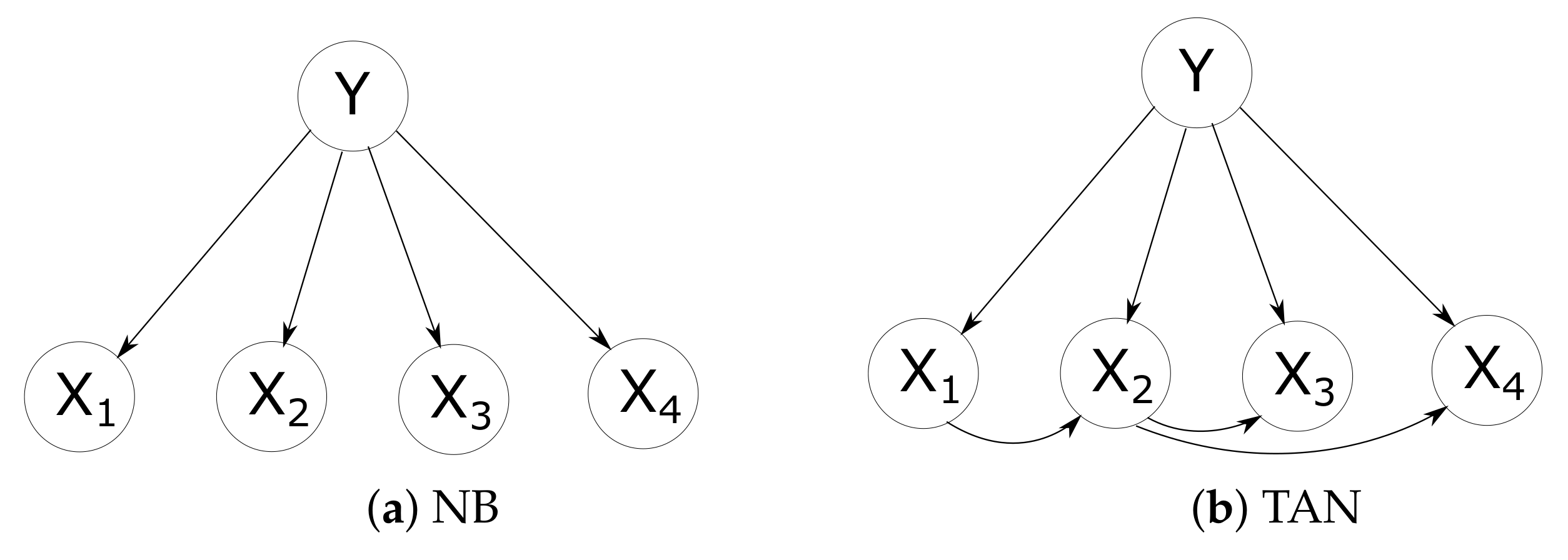
2.1. Bayesian Network Classifiers
2.2. Tree Augmented Naive Bayes
- 1.
- Compute between each pair of attributes, , from the training data.
- 2.
- Build a complete undirected graph in which the nodes are the attributes . Annotate the weight of an edge connecting to by .
- 3.
- Build a maximum weighted spanning tree.
- 4.
- Transform the resulting undirected tree to a directed one by choosing a root variable and setting the direction of all edges to be outward from it, thus getting the parent node of node .
- 5.
- Construct a TAN model by adding a node labelled by Y and adding an arc from Y to each .
3. Attribute Selective Tree-Augmented Naive Bayes
3.1. Motivation
3.2. Building Model Sequence
3.3. Ranking the Attributes
- 1.
- Mutual Information (MI) (Mutual information measures the amount of information shared by two variables. This can also be interpreted as the amount of information that one variable provides about another) is an intuitive score since it is a measure of correlation between an attribute and the class variable. Before we present the definition of mutual information, we would first present the concepts of entropy and conditional entropy. The entropy of a random variable x is defined asThe conditional entropy of X given Y isThe mutual information between X and Y is defined as the difference between the entropy and the conditional entropyThis heuristic considers a score for each attribute independently of others.
- 2.
- Symmetrical Uncertainty (SU) (Symmetrical uncertainty is the normalized mutual information. The range of symmetrical uncertainty is , where the value 1 indicates that knowledge of the value of either one completely predicts the value of the other and the value 0 indicates that the two variables are independent) [23] can be interpreted as a sort of mutual information normalized to interval [0, 1]:It is obvious that mutual information is biased in favor of attributes with more values and so large entropy. However, symmetrical uncertainty, which is normalized to the range , is an unbiased metric and ensures they are comparable and have the same effect. As a result, we can expect to obtain a more appropriate ranking of attributes based on symmetrical uncertainty.
- 3.
- Minimum Redundancy-Maximum Relevance (MRMR) criterion (MRMR, short for Minimum Reduncancy-Maximum Relevance, always tries to select the attribute which has the best trade off between the relevance to the class variable and the the averaged redundancy to the attributes already selected), which was proposed by Peng et al. [24], not only considers mutual information to ensure feature relevance, but introduces a penalty to enforce low correlations with features already selected. MRMR is very similar to Mutual Information Feature Selection (MIFS) [25], except that the latter replace with a more general configurable parameter , where k means the number of the attributes that have been selected so far, and is also the number of steps. Assume at step k, the attribute set selected so far is , while is the set difference between the original set of inputs and . The attribute returned by MRMR criterion at step is,At each step, this strategy selected the variable which has the best trade off between the relevance of X to the class Y and the averaged redundancy of X to the selected attributes .
- 4.
- Conditional Mutual Information Maximization (CMIM) (CMIM, short for Conditional Mutual Information Maximization, tries to select the attribute that maximizes the minimal mutual information with the class within the attributes already selected) proposes to select the feature whose minimal relevance conditioned to the selected attributes is maximal. This heuristic was proposed by Fleuret [26] and also later by Chen et al. [27] as direct rank (dRank). CMIM computes the mutual information of X and the class variable Y, conditioned on each attribute previously selected. Then the minimal value is retained and the attribute that has a maximal minimal conditional relevance is selected.In formal notation, the variable returned at step according to the CMIM strategy is
- 5.
- Joint Mutual Information (JMI) (JMI, short for joint Mutual Information, tries to select the attribute which is complementary most with existing attributes), which was proposed by Yang and Moody [28] and also later by Meyer et al. [29], tries to select a candidate attribute if it is complementary with existing attributes. As a result, JMI focuses on increasing the complementary information between attributes. The variable returned by JMI criterion at step isThe score in JMI is the information between the class variable and a random variable, defined by pairing the candidate X with each attribute previously selected.
3.4. Cross Validation Risk Minimization
| Algorithm 1 Training algorithm of attribute selective TAN. |
|
4. Experiments and Analysis
4.1. Experimental Methodology
- 1.
- Missing values are considered as a distinct value rather than replaced with modes and means for nominal and numeric attributes as in the Weka software.
- 2.
- Root mean squared error is calculated exclusively on the true class label. This is different from Weka’s implementation, where all class labels are considered.
4.2. Win/Draw/Loss Analysis
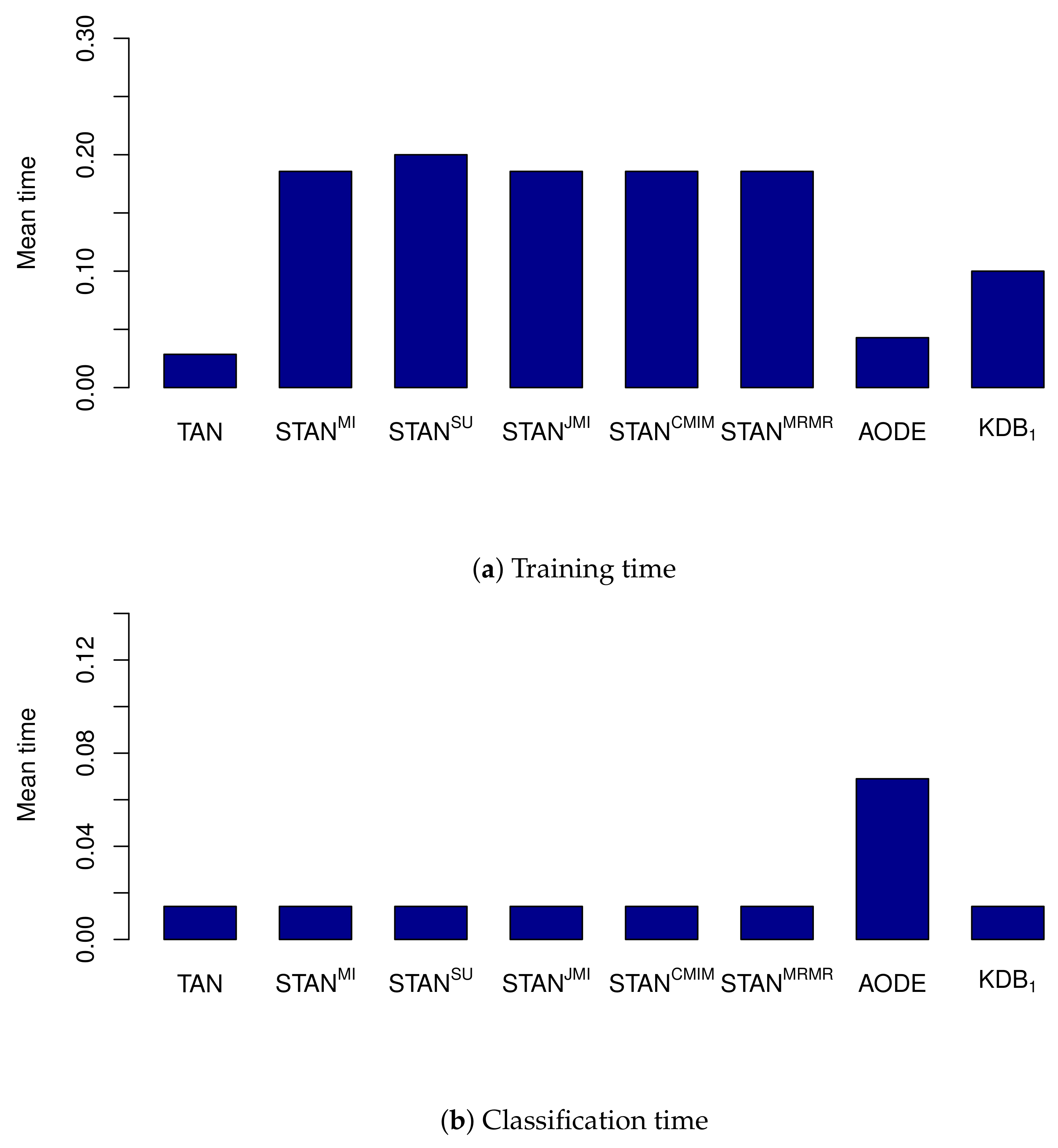
4.3. Analysis of Training and Classification Time
5. Discussion
- STAN algorithms with different ranking strategies achieve superior classification performance than regular TAN at the cost of a modest increase in training time.
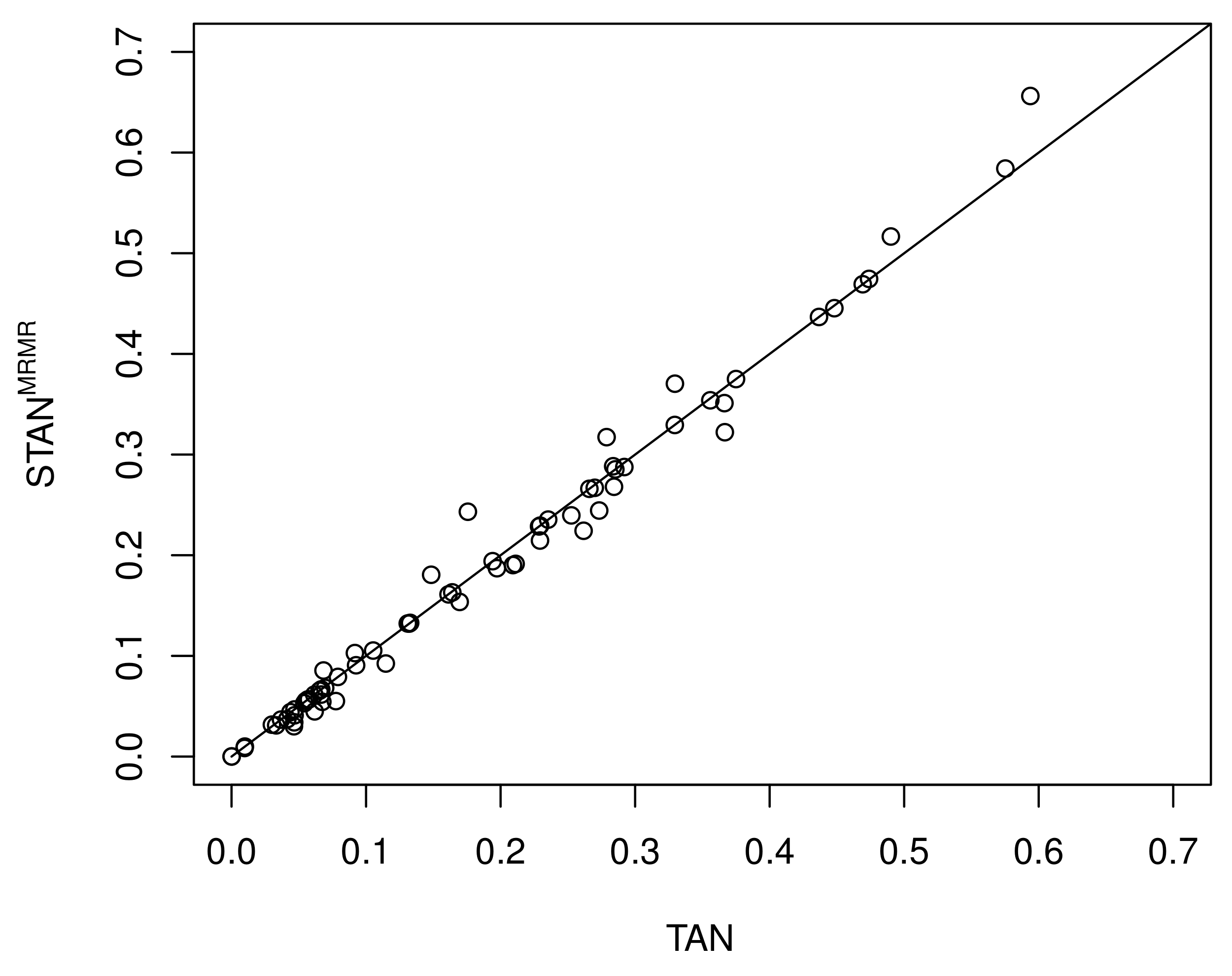
- MRMR ranking strategy achieves the best classification performance compared to other ranking strategies, and the advantage over regular TAN is significant.
- STAN with MRMR ranking strategy is comparable with AODE and superior to KDB in terms of accuracy, while requires less classification time than AODE.
Author Contributions
Funding
Institutional Review Board Statement
Informed Consent Statement
Data Availability Statement
Acknowledgments
Conflicts of Interest
Appendix A

| Dataset | TAN | STANMI | STANSU | STANJMI | STANCMIM | STANMRMR | AODE | KDB1 |
|---|---|---|---|---|---|---|---|---|
| contact-lenses | 0.3750 ± 0.3758 | 0.3750 ± 0.3425 | 0.3750 ± 0.3425 | 0.3750 ± 0.3425 | 0.3750 ± 0.3425 | 0.3750 ± 0.3425 | 0.4167 ± 0.3574 | 0.2917 ± 0.3543 |
| lung-cancer | 0.5938 ± 0.2265 | 0.6875 ± 0.2641 | 0.7188 ± 0.2502 | 0.5625 ± 0.3289 | 0.6250 ± 0.2605 | 0.6562 ± 0.2733 | 0.4688 ± 0.2885 | 0.5938 ± 0.3082 |
| labor-negotiations | 0.1053 ± 0.1234 | 0.1053 ± 0.1234 | 0.0877 ± 0.1272 | 0.1053 ± 0.1234 | 0.1228 ± 0.2090 | 0.1053 ± 0.1234 | 0.0526 ± 0.0675 | 0.1053 ± 0.1146 |
| post-operative | 0.3667 ± 0.2075 | 0.3222 ± 0.2117 | 0.3444 ± 0.2124 | 0.3111 ± 0.1663 | 0.3111 ± 0.1663 | 0.3222 ± 0.2263 | 0.3444 ± 0.1882 | 0.3444 ± 0.1748 |
| zoo | 0.0099 ± 0.0527 | 0.0099 ± 0.0527 | 0.0099 ± 0.0527 | 0.0099 ± 0.0527 | 0.0198 ± 0.0542 | 0.0099 ± 0.0527 | 0.0198 ± 0.0384 | 0.0495 ± 0.0614 |
| promoters | 0.1321 ± 0.1036 | 0.1792 ± 0.1307 | 0.1887 ± 0.1251 | 0.1792 ± 0.1280 | 0.1604 ± 0.1072 | 0.1321 ± 0.1108 | 0.1038 ± 0.0648 | 0.1321 ± 0.0891 |
| echocardiogram | 0.3664 ± 0.1549 | 0.3893 ± 0.1191 | 0.3664 ± 0.0922 | 0.3969 ± 0.0998 | 0.3969 ± 0.0998 | 0.3511 ± 0.1132 | 0.3435 ± 0.1143 | 0.3664 ± 0.1511 |
| lymphography | 0.1757 ± 0.1003 | 0.1622 ± 0.1007 | 0.1689 ± 0.1005 | 0.1622 ± 0.1007 | 0.1689 ± 0.1047 | 0.2432 ± 0.1177 | 0.1486 ± 0.0991 | 0.1757 ± 0.0791 |
| iris | 0.0667 ± 0.0632 | 0.0667 ± 0.0632 | 0.0667 ± 0.0632 | 0.0667 ± 0.0632 | 0.0667 ± 0.0632 | 0.0667 ± 0.0632 | 0.0600 ± 0.0655 | 0.0733 ± 0.0505 |
| teaching-ae | 0.4901 ± 0.1245 | 0.4901 ± 0.1245 | 0.4901 ± 0.1245 | 0.5232 ± 0.1216 | 0.5232 ± 0.1216 | 0.5166 ± 0.1436 | 0.4834 ± 0.1179 | 0.4834 ± 0.1079 |
| hepatitis | 0.1484 ± 0.1280 | 0.1548 ± 0.1246 | 0.1548 ± 0.1264 | 0.1484 ± 0.1280 | 0.1484 ± 0.1264 | 0.1806 ± 0.1236 | 0.1935 ± 0.1244 | 0.2194 ± 0.1205 |
| wine | 0.0618 ± 0.0643 | 0.0562 ± 0.0534 | 0.0562 ± 0.0534 | 0.0618 ± 0.0647 | 0.0674 ± 0.0611 | 0.0449 ± 0.0532 | 0.0281 ± 0.0404 | 0.0674 ± 0.0633 |
| autos | 0.2293 ± 0.1374 | 0.1951 ± 0.1278 | 0.2000 ± 0.1118 | 0.2098 ± 0.1067 | 0.1951 ± 0.1162 | 0.2146 ± 0.1230 | 0.2537 ± 0.1104 | 0.2293 ± 0.1374 |
| sonar | 0.2788 ± 0.0840 | 0.3029 ± 0.1086 | 0.3029 ± 0.1086 | 0.2981 ± 0.0925 | 0.2692 ± 0.1032 | 0.3173 ± 0.1301 | 0.1394 ± 0.0888 | 0.2548 ± 0.0914 |
| glass-id | 0.2617 ± 0.0944 | 0.2664 ± 0.0923 | 0.2290 ± 0.0757 | 0.2523 ± 0.0944 | 0.2523 ± 0.0944 | 0.2243 ± 0.0671 | 0.1589 ± 0.0576 | 0.2383 ± 0.0720 |
| new-thyroid | 0.0791 ± 0.0647 | 0.0791 ± 0.0647 | 0.0791 ± 0.0647 | 0.0791 ± 0.0647 | 0.0791 ± 0.0647 | 0.0791 ± 0.0647 | 0.0512 ± 0.0544 | 0.0651 ± 0.0454 |
| audio | 0.2920 ± 0.0926 | 0.3053 ± 0.0676 | 0.3053 ± 0.0676 | 0.3009 ± 0.0851 | 0.3009 ± 0.0934 | 0.2876 ± 0.0821 | 0.2301 ± 0.0649 | 0.3097 ± 0.1054 |
| hungarian | 0.1973 ± 0.0606 | 0.2041 ± 0.0613 | 0.2109 ± 0.0708 | 0.1973 ± 0.0524 | 0.1905 ± 0.0511 | 0.1871 ± 0.0789 | 0.1429 ± 0.0676 | 0.2075 ± 0.0625 |
| heart-disease-c | 0.2112 ± 0.1005 | 0.2211 ± 0.1154 | 0.2244 ± 0.1037 | 0.2178 ± 0.1020 | 0.2079 ± 0.1081 | 0.1914 ± 0.0820 | 0.1848 ± 0.1067 | 0.2178 ± 0.1428 |
| haberman | 0.2843 ± 0.1023 | 0.2778 ± 0.0868 | 0.2778 ± 0.0868 | 0.2745 ± 0.0851 | 0.2745 ± 0.0851 | 0.2680 ± 0.0985 | 0.2712 ± 0.1188 | 0.2778 ± 0.1024 |
| primary-tumor | 0.5752 ± 0.0960 | 0.5841 ± 0.1188 | 0.5841 ± 0.1188 | 0.5841 ± 0.1188 | 0.5782 ± 0.1209 | 0.5841 ± 0.1184 | 0.5162 ± 0.0984 | 0.5841 ± 0.1119 |
| ionosphere | 0.0684 ± 0.0510 | 0.0741 ± 0.0453 | 0.0769 ± 0.0448 | 0.0741 ± 0.0542 | 0.0712 ± 0.0409 | 0.0855 ± 0.0428 | 0.0826 ± 0.0405 | 0.0684 ± 0.0441 |
| dermatology | 0.0464 ± 0.0390 | 0.0383 ± 0.0345 | 0.0437 ± 0.0359 | 0.0410 ± 0.0287 | 0.0437 ± 0.0378 | 0.0301 ± 0.0282 | 0.0219 ± 0.0275 | 0.0301 ± 0.0258 |
| horse-colic | 0.2092 ± 0.0629 | 0.1875 ± 0.0524 | 0.1793 ± 0.0567 | 0.1793 ± 0.0715 | 0.1685 ± 0.0618 | 0.1902 ± 0.0604 | 0.2038 ± 0.0590 | 0.2120 ± 0.0615 |
| house-votes-84 | 0.0552 ± 0.0375 | 0.0644 ± 0.0386 | 0.0644 ± 0.0386 | 0.0552 ± 0.0315 | 0.0529 ± 0.0404 | 0.0552 ± 0.0368 | 0.0529 ± 0.0346 | 0.0690 ± 0.0353 |
| cylinder-bands | 0.3296 ± 0.0719 | 0.3833 ± 0.0730 | 0.3796 ± 0.0821 | 0.3722 ± 0.0634 | 0.3759 ± 0.0677 | 0.3704 ± 0.0774 | 0.1611 ± 0.0421 | 0.2074 ± 0.0575 |
| chess | 0.0926 ± 0.0492 | 0.0907 ± 0.0509 | 0.0907 ± 0.0509 | 0.0944 ± 0.0553 | 0.0907 ± 0.0509 | 0.0907 ± 0.0509 | 0.1053 ± 0.0631 | 0.0998 ± 0.0354 |
| syncon | 0.0300 ± 0.0249 | 0.0283 ± 0.0241 | 0.0283 ± 0.0241 | 0.0317 ± 0.0266 | 0.0267 ± 0.0235 | 0.0317 ± 0.0291 | 0.0200 ± 0.0163 | 0.0200 ± 0.0156 |
| balance-scale | 0.1328 ± 0.0156 | 0.1328 ± 0.0156 | 0.1328 ± 0.0156 | 0.1328 ± 0.0156 | 0.1328 ± 0.0156 | 0.1328 ± 0.0156 | 0.1120 ± 0.0159 | 0.1424 ± 0.0307 |
| soybean | 0.0469 ± 0.0136 | 0.0586 ± 0.0195 | 0.0571 ± 0.0180 | 0.0469 ± 0.0158 | 0.0454 ± 0.0100 | 0.0410 ± 0.0095 | 0.0542 ± 0.0184 | 0.0644 ± 0.0205 |
| credit-a | 0.1696 ± 0.0370 | 0.1667 ± 0.0394 | 0.1623 ± 0.0374 | 0.1739 ± 0.0460 | 0.1696 ± 0.0444 | 0.1536 ± 0.0377 | 0.1261 ± 0.0210 | 0.1696 ± 0.0417 |
| breast-cancer-w | 0.0415 ± 0.0273 | 0.0443 ± 0.0252 | 0.0429 ± 0.0271 | 0.0415 ± 0.0271 | 0.0386 ± 0.0207 | 0.0372 ± 0.0237 | 0.0386 ± 0.0248 | 0.0486 ± 0.0181 |
| pima-ind-diabetes | 0.2526 ± 0.0509 | 0.2487 ± 0.0416 | 0.2487 ± 0.0416 | 0.2409 ± 0.0505 | 0.2461 ± 0.0480 | 0.2396 ± 0.0550 | 0.2513 ± 0.0636 | 0.2578 ± 0.0583 |
| vehicle | 0.2837 ± 0.0603 | 0.3014 ± 0.0505 | 0.3014 ± 0.0505 | 0.3121 ± 0.0479 | 0.2837 ± 0.0570 | 0.2884 ± 0.0654 | 0.3132 ± 0.0563 | 0.3026 ± 0.0627 |
| anneal | 0.0468 ± 0.0182 | 0.0468 ± 0.0182 | 0.0468 ± 0.0182 | 0.0468 ± 0.0182 | 0.0468 ± 0.0182 | 0.0468 ± 0.0182 | 0.0735 ± 0.0232 | 0.0445 ± 0.0156 |
| tic-tac-toe | 0.2286 ± 0.0395 | 0.2286 ± 0.0395 | 0.2286 ± 0.0395 | 0.2286 ± 0.0395 | 0.2286 ± 0.0395 | 0.2286 ± 0.0395 | 0.2683 ± 0.0432 | 0.2463 ± 0.0382 |
| vowel | 0.0667 ± 0.0259 | 0.0616 ± 0.0284 | 0.0616 ± 0.0284 | 0.0646 ± 0.0270 | 0.0707 ± 0.0354 | 0.0616 ± 0.0284 | 0.0808 ± 0.0296 | 0.2162 ± 0.0272 |
| german | 0.2700 ± 0.0515 | 0.2750 ± 0.0411 | 0.2760 ± 0.0470 | 0.2770 ± 0.0653 | 0.2740 ± 0.0604 | 0.2670 ± 0.0398 | 0.2410 ± 0.0535 | 0.2660 ± 0.0634 |
| led | 0.2660 ± 0.0569 | 0.2660 ± 0.0569 | 0.2660 ± 0.0569 | 0.2660 ± 0.0569 | 0.2660 ± 0.0569 | 0.2660 ± 0.0569 | 0.2700 ± 0.0604 | 0.2640 ± 0.0603 |
| contraceptive-mc | 0.4739 ± 0.0345 | 0.4800 ± 0.0328 | 0.4779 ± 0.0318 | 0.4793 ± 0.0333 | 0.4739 ± 0.0234 | 0.4745 ± 0.0266 | 0.4671 ± 0.0455 | 0.4684 ± 0.0276 |
| yeast | 0.4481 ± 0.0360 | 0.4481 ± 0.0360 | 0.4461 ± 0.0324 | 0.4481 ± 0.0360 | 0.4481 ± 0.0360 | 0.4454 ± 0.0322 | 0.4205 ± 0.0402 | 0.4394 ± 0.0326 |
| volcanoes | 0.3559 ± 0.0250 | 0.3539 ± 0.0276 | 0.3539 ± 0.0276 | 0.3533 ± 0.0294 | 0.3533 ± 0.0294 | 0.3539 ± 0.0276 | 0.3539 ± 0.0331 | 0.3520 ± 0.0258 |
| car | 0.0567 ± 0.0182 | 0.0567 ± 0.0182 | 0.0567 ± 0.0182 | 0.0567 ± 0.0182 | 0.0567 ± 0.0182 | 0.0567 ± 0.0182 | 0.0845 ± 0.0193 | 0.0567 ± 0.0182 |
| segment | 0.0615 ± 0.0142 | 0.0610 ± 0.0133 | 0.0610 ± 0.0133 | 0.0610 ± 0.0133 | 0.0610 ± 0.0133 | 0.0615 ± 0.0130 | 0.0563 ± 0.0091 | 0.0567 ± 0.0158 |
| hypothyroid | 0.0332 ± 0.0126 | 0.0319 ± 0.0110 | 0.0322 ± 0.0098 | 0.0326 ± 0.0104 | 0.0316 ± 0.0106 | 0.0310 ± 0.0095 | 0.0348 ± 0.0118 | 0.0338 ± 0.0137 |
| splice-c4.5 | 0.0466 ± 0.0129 | 0.0349 ± 0.0089 | 0.0349 ± 0.0089 | 0.0349 ± 0.0102 | 0.0318 ± 0.0078 | 0.0340 ± 0.0088 | 0.0375 ± 0.0087 | 0.0482 ± 0.0152 |
| kr-vs-kp | 0.0776 ± 0.0228 | 0.0569 ± 0.0186 | 0.0579 ± 0.0187 | 0.0569 ± 0.0186 | 0.0607 ± 0.0145 | 0.0551 ± 0.0142 | 0.0854 ± 0.0187 | 0.0544 ± 0.0171 |
| abalone | 0.4692 ± 0.0285 | 0.4692 ± 0.0285 | 0.4692 ± 0.0285 | 0.4692 ± 0.0285 | 0.4690 ± 0.0279 | 0.4692 ± 0.0285 | 0.4551 ± 0.0214 | 0.4656 ± 0.0237 |
| spambase | 0.0696 ± 0.0106 | 0.0689 ± 0.0115 | 0.0685 ± 0.0118 | 0.0696 ± 0.0106 | 0.0689 ± 0.0112 | 0.0682 ± 0.0114 | 0.0635 ± 0.0114 | 0.0702 ± 0.0121 |
| phoneme | 0.2733 ± 0.0177 | 0.2413 ± 0.0119 | 0.2413 ± 0.0119 | 0.2413 ± 0.0119 | 0.2413 ± 0.0119 | 0.2444 ± 0.0119 | 0.2100 ± 0.0144 | 0.2120 ± 0.0123 |
| wall-following | 0.1147 ± 0.0116 | 0.0872 ± 0.0092 | 0.0872 ± 0.0092 | 0.0867 ± 0.0097 | 0.0861 ± 0.0108 | 0.0924 ± 0.0110 | 0.1514 ± 0.0101 | 0.1043 ± 0.0094 |
| page-blocks | 0.0541 ± 0.0100 | 0.0530 ± 0.0081 | 0.0530 ± 0.0081 | 0.0541 ± 0.0100 | 0.0550 ± 0.0099 | 0.0530 ± 0.0081 | 0.0502 ± 0.0066 | 0.0590 ± 0.0102 |
| optdigits | 0.0438 ± 0.0064 | 0.0441 ± 0.0064 | 0.0441 ± 0.0064 | 0.0441 ± 0.0064 | 0.0443 ± 0.0068 | 0.0441 ± 0.0067 | 0.0283 ± 0.0095 | 0.0454 ± 0.0070 |
| satellite | 0.1310 ± 0.0126 | 0.1321 ± 0.0118 | 0.1321 ± 0.0118 | 0.1318 ± 0.0126 | 0.1340 ± 0.0135 | 0.1322 ± 0.0132 | 0.1301 ± 0.0131 | 0.1392 ± 0.0135 |
| musk2 | 0.0917 ± 0.0086 | 0.1003 ± 0.0142 | 0.1073 ± 0.0165 | 0.0996 ± 0.0146 | 0.0997 ± 0.0187 | 0.1028 ± 0.0127 | 0.1511 ± 0.0101 | 0.0867 ± 0.0097 |
| mushrooms | 0.0001 ± 0.0004 | 0.0001 ± 0.0004 | 0.0001 ± 0.0004 | 0.0001 ± 0.0004 | 0.0000 ± 0.0000 | 0.0001 ± 0.0004 | 0.0002 ± 0.0005 | 0.0006 ± 0.0009 |
| thyroid | 0.2294 ± 0.0111 | 0.2294 ± 0.0111 | 0.2301 ± 0.0121 | 0.2294 ± 0.0111 | 0.2294 ± 0.0111 | 0.2294 ± 0.0111 | 0.2421 ± 0.0136 | 0.2319 ± 0.0146 |
| pendigits | 0.0576 ± 0.0064 | 0.0576 ± 0.0064 | 0.0576 ± 0.0064 | 0.0552 ± 0.0056 | 0.0544 ± 0.0058 | 0.0568 ± 0.0064 | 0.0254 ± 0.0029 | 0.0529 ± 0.0066 |
| sign | 0.2853 ± 0.0094 | 0.2853 ± 0.0094 | 0.2853 ± 0.0094 | 0.2853 ± 0.0094 | 0.2853 ± 0.0094 | 0.2853 ± 0.0094 | 0.2960 ± 0.0119 | 0.3055 ± 0.0140 |
| nursery | 0.0654 ± 0.0062 | 0.0654 ± 0.0062 | 0.0654 ± 0.0062 | 0.0654 ± 0.0062 | 0.0654 ± 0.0062 | 0.0654 ± 0.0062 | 0.0733 ± 0.0059 | 0.0654 ± 0.0061 |
| magic | 0.1613 ± 0.0076 | 0.1611 ± 0.0086 | 0.1611 ± 0.0086 | 0.1613 ± 0.0076 | 0.1613 ± 0.0076 | 0.1611 ± 0.0076 | 0.1726 ± 0.0084 | 0.1759 ± 0.0107 |
| letter-recog | 0.1941 ± 0.0085 | 0.1941 ± 0.0085 | 0.1941 ± 0.0085 | 0.1941 ± 0.0085 | 0.1941 ± 0.0085 | 0.1941 ± 0.0085 | 0.1514 ± 0.0089 | 0.1920 ± 0.0112 |
| adult | 0.1641 ± 0.0037 | 0.1609 ± 0.0040 | 0.1609 ± 0.0040 | 0.1635 ± 0.0034 | 0.1642 ± 0.0037 | 0.1631 ± 0.0045 | 0.1679 ± 0.0032 | 0.1638 ± 0.0044 |
| shuttle | 0.0097 ± 0.0013 | 0.0085 ± 0.0013 | 0.0085 ± 0.0013 | 0.0085 ± 0.0013 | 0.0085 ± 0.0013 | 0.0085 ± 0.0013 | 0.0101 ± 0.0010 | 0.0163 ± 0.0012 |
| connect-4 | 0.2354 ± 0.0050 | 0.2354 ± 0.0050 | 0.2354 ± 0.0050 | 0.2354 ± 0.0050 | 0.2354 ± 0.0050 | 0.2354 ± 0.0050 | 0.2422 ± 0.0047 | 0.2406 ± 0.0030 |
| waveform | 0.0368 ± 0.0015 | 0.0370 ± 0.0014 | 0.0370 ± 0.0014 | 0.0369 ± 0.0014 | 0.0369 ± 0.0014 | 0.0367 ± 0.0015 | 0.0343 ± 0.0008 | 0.0396 ± 0.0021 |
| localization | 0.4367 ± 0.0033 | 0.4367 ± 0.0033 | 0.4367 ± 0.0033 | 0.4367 ± 0.0033 | 0.4367 ± 0.0033 | 0.4367 ± 0.0033 | 0.4333 ± 0.0027 | 0.4642 ± 0.0040 |
| census-income | 0.0675 ± 0.0016 | 0.0585 ± 0.0020 | 0.0571 ± 0.0010 | 0.0567 ± 0.0010 | 0.0599 ± 0.0011 | 0.0544 ± 0.0015 | 0.1106 ± 0.0015 | 0.0667 ± 0.0014 |
| poker-hand | 0.3295 ± 0.0015 | 0.3294 ± 0.0015 | 0.3294 ± 0.0015 | 0.3294 ± 0.0015 | 0.3294 ± 0.0015 | 0.3294 ± 0.0015 | 0.4812 ± 0.0028 | 0.3291 ± 0.0012 |
| donation | 0.0001 ± 0.0000 | 0.0001 ± 0.0000 | 0.0001 ± 0.0000 | 0.0001 ± 0.0000 | 0.0001 ± 0.0000 | 0.0001 ± 0.0000 | 0.0002 ± 0.0000 | 0.0001 ± 0.0000 |
| Dataset | TAN | STANMI | STANSU | STANJMI | STANCMIM | STANMRMR | AODE | KDB1 |
|---|---|---|---|---|---|---|---|---|
| contact-lenses | 0.6077 ± 0.1831 | 0.5438 ± 0.2091 | 0.5438 ± 0.2091 | 0.5635 ± 0.2278 | 0.5438 ± 0.2091 | 0.5635 ± 0.2278 | 0.5226 ± 0.2221 | 0.5024 ± 0.2104 |
| lung-cancer | 0.7623 ± 0.1357 | 0.8044 ± 0.1515 | 0.7955 ± 0.1412 | 0.6807 ± 0.2643 | 0.7364 ± 0.1709 | 0.7690 ± 0.1463 | 0.6614 ± 0.2444 | 0.7523 ± 0.2928 |
| labor-negotiations | 0.2935 ± 0.1975 | 0.2988 ± 0.2081 | 0.2847 ± 0.2132 | 0.2877 ± 0.1972 | 0.3131 ± 0.2514 | 0.2915 ± 0.2033 | 0.2104 ± 0.1455 | 0.3014 ± 0.1907 |
| post-operative | 0.5340 ± 0.1393 | 0.5153 ± 0.1354 | 0.5206 ± 0.1241 | 0.5017 ± 0.1150 | 0.5017 ± 0.1150 | 0.5133 ± 0.1405 | 0.5136 ± 0.1059 | 0.5289 ± 0.1031 |
| zoo | 0.1309 ± 0.1131 | 0.1168 ± 0.1054 | 0.1168 ± 0.1054 | 0.1144 ± 0.1052 | 0.1477 ± 0.1144 | 0.1397 ± 0.1139 | 0.1344 ± 0.0935 | 0.1984 ± 0.1255 |
| promoters | 0.3264 ± 0.1659 | 0.3883 ± 0.1721 | 0.3895 ± 0.1698 | 0.3864 ± 0.1749 | 0.3702 ± 0.1647 | 0.3485 ± 0.1748 | 0.2795 ± 0.0940 | 0.3292 ± 0.1603 |
| echocardiogram | 0.5276 ± 0.1017 | 0.5144 ± 0.0890 | 0.4999 ± 0.0640 | 0.5073 ± 0.0741 | 0.5073 ± 0.0741 | 0.4986 ± 0.0693 | 0.4829 ± 0.0808 | 0.5288 ± 0.1034 |
| lymphography | 0.3813 ± 0.1227 | 0.3816 ± 0.1231 | 0.3891 ± 0.1250 | 0.3814 ± 0.1230 | 0.3874 ± 0.1175 | 0.4369 ± 0.0996 | 0.3274 ± 0.1395 | 0.3726 ± 0.1169 |
| iris | 0.2211 ± 0.1353 | 0.2211 ± 0.1353 | 0.2211 ± 0.1353 | 0.2211 ± 0.1353 | 0.2211 ± 0.1353 | 0.2211 ± 0.1353 | 0.2224 ± 0.1303 | 0.2273 ± 0.1252 |
| teaching-ae | 0.6189 ± 0.0671 | 0.6189 ± 0.0671 | 0.6189 ± 0.0671 | 0.6272 ± 0.0834 | 0.6272 ± 0.0834 | 0.6404 ± 0.0749 | 0.6105 ± 0.0684 | 0.6224 ± 0.0683 |
| hepatitis | 0.3434 ± 0.1479 | 0.3530 ± 0.1396 | 0.3409 ± 0.1326 | 0.3416 ± 0.1422 | 0.3475 ± 0.1459 | 0.3751 ± 0.1442 | 0.3711 ± 0.1079 | 0.4188 ± 0.1082 |
| wine | 0.2026 ± 0.1223 | 0.2020 ± 0.1179 | 0.2063 ± 0.1234 | 0.2142 ± 0.1218 | 0.2202 ± 0.1180 | 0.1923 ± 0.1029 | 0.1528 ± 0.1007 | 0.2210 ± 0.0927 |
| autos | 0.4725 ± 0.1291 | 0.4214 ± 0.1637 | 0.4241 ± 0.1350 | 0.4339 ± 0.1327 | 0.4312 ± 0.1356 | 0.4350 ± 0.1427 | 0.4760 ± 0.1102 | 0.4736 ± 0.1286 |
| sonar | 0.4856 ± 0.0890 | 0.5085 ± 0.1087 | 0.5085 ± 0.1087 | 0.5027 ± 0.0989 | 0.4805 ± 0.0920 | 0.5161 ± 0.1172 | 0.3349 ± 0.1109 | 0.4629 ± 0.0783 |
| glass-id | 0.4360 ± 0.0585 | 0.4504 ± 0.0608 | 0.4286 ± 0.0604 | 0.4381 ± 0.0594 | 0.4371 ± 0.0583 | 0.4170 ± 0.0587 | 0.3654 ± 0.0546 | 0.4199 ± 0.0650 |
| new-thyroid | 0.2554 ± 0.0991 | 0.2554 ± 0.0991 | 0.2554 ± 0.0991 | 0.2554 ± 0.0991 | 0.2554 ± 0.0991 | 0.2554 ± 0.0991 | 0.2221 ± 0.0850 | 0.2262 ± 0.0710 |
| audio | 0.5212 ± 0.0855 | 0.5168 ± 0.0663 | 0.5175 ± 0.0660 | 0.5151 ± 0.0803 | 0.5139 ± 0.0809 | 0.5136 ± 0.0672 | 0.4639 ± 0.0606 | 0.5294 ± 0.0939 |
| hungarian | 0.3895 ± 0.0711 | 0.3882 ± 0.0740 | 0.3816 ± 0.0684 | 0.3855 ± 0.0610 | 0.3870 ± 0.0548 | 0.3778 ± 0.0628 | 0.3506 ± 0.0845 | 0.3917 ± 0.0684 |
| heart-disease-c | 0.4177 ± 0.0861 | 0.4203 ± 0.0881 | 0.4159 ± 0.0778 | 0.4171 ± 0.0820 | 0.4152 ± 0.0810 | 0.3874 ± 0.0692 | 0.3605 ± 0.0844 | 0.4135 ± 0.0989 |
| haberman | 0.4433 ± 0.0759 | 0.4299 ± 0.0756 | 0.4299 ± 0.0756 | 0.4280 ± 0.0743 | 0.4280 ± 0.0743 | 0.4283 ± 0.0728 | 0.4402 ± 0.0820 | 0.4416 ± 0.0776 |
| primary-tumor | 0.7280 ± 0.0579 | 0.7272 ± 0.0574 | 0.7264 ± 0.0610 | 0.7272 ± 0.0574 | 0.7266 ± 0.0580 | 0.7258 ± 0.0572 | 0.6972 ± 0.0585 | 0.7250 ± 0.0589 |
| ionosphere | 0.2573 ± 0.1077 | 0.2616 ± 0.0991 | 0.2654 ± 0.0981 | 0.2596 ± 0.1044 | 0.2452 ± 0.0947 | 0.2638 ± 0.0941 | 0.2841 ± 0.0724 | 0.2434 ± 0.1047 |
| dermatology | 0.1826 ± 0.0695 | 0.1792 ± 0.0745 | 0.1786 ± 0.0719 | 0.1786 ± 0.0633 | 0.1878 ± 0.0793 | 0.1576 ± 0.0593 | 0.1145 ± 0.0617 | 0.1521 ± 0.0784 |
| horse-colic | 0.4289 ± 0.0672 | 0.3829 ± 0.0585 | 0.3714 ± 0.0569 | 0.3746 ± 0.0593 | 0.3764 ± 0.0587 | 0.3879 ± 0.0520 | 0.4029 ± 0.0709 | 0.4185 ± 0.0597 |
| house-votes-84 | 0.2181 ± 0.0792 | 0.2337 ± 0.0803 | 0.2337 ± 0.0803 | 0.2161 ± 0.0663 | 0.2123 ± 0.0789 | 0.2115 ± 0.0686 | 0.2016 ± 0.0736 | 0.2235 ± 0.0721 |
| cylinder-bands | 0.4405 ± 0.0420 | 0.4407 ± 0.0282 | 0.4393 ± 0.0280 | 0.4365 ± 0.0278 | 0.4423 ± 0.0281 | 0.4436 ± 0.0246 | 0.3656 ± 0.0451 | 0.4312 ± 0.0590 |
| chess | 0.2594 ± 0.0470 | 0.2589 ± 0.0477 | 0.2590 ± 0.0475 | 0.2613 ± 0.0495 | 0.2597 ± 0.0479 | 0.2590 ± 0.0475 | 0.2855 ± 0.0485 | 0.2671 ± 0.0384 |
| syncon | 0.1602 ± 0.0688 | 0.1608 ± 0.0807 | 0.1608 ± 0.0807 | 0.1651 ± 0.0748 | 0.1557 ± 0.0862 | 0.1617 ± 0.0800 | 0.1287 ± 0.0448 | 0.1271 ± 0.0686 |
| balance-scale | 0.3971 ± 0.0186 | 0.3971 ± 0.0186 | 0.3971 ± 0.0186 | 0.3971 ± 0.0186 | 0.3971 ± 0.0186 | 0.3971 ± 0.0186 | 0.3999 ± 0.0234 | 0.4014 ± 0.0200 |
| soybean | 0.2014 ± 0.0341 | 0.2139 ± 0.0365 | 0.2062 ± 0.0347 | 0.1914 ± 0.0294 | 0.1945 ± 0.0337 | 0.1828 ± 0.0265 | 0.2224 ± 0.0402 | 0.2206 ± 0.0436 |
| credit-a | 0.3704 ± 0.0443 | 0.3404 ± 0.0242 | 0.3377 ± 0.0396 | 0.3386 ± 0.0314 | 0.3371 ± 0.0334 | 0.3473 ± 0.0307 | 0.3164 ± 0.0387 | 0.3692 ± 0.0419 |
| breast-cancer-w | 0.1928 ± 0.0618 | 0.1877 ± 0.0544 | 0.1931 ± 0.0595 | 0.1794 ± 0.0566 | 0.1830 ± 0.0475 | 0.1746 ± 0.0527 | 0.1778 ± 0.0879 | 0.1951 ± 0.0461 |
| pima-ind-diabetes | 0.4225 ± 0.0442 | 0.4142 ± 0.0496 | 0.4142 ± 0.0496 | 0.4116 ± 0.0516 | 0.4114 ± 0.0501 | 0.4079 ± 0.0495 | 0.4071 ± 0.0438 | 0.4212 ± 0.0494 |
| vehicle | 0.4638 ± 0.0458 | 0.4691 ± 0.0389 | 0.4691 ± 0.0389 | 0.4706 ± 0.0387 | 0.4634 ± 0.0448 | 0.4611 ± 0.0425 | 0.4653 ± 0.0343 | 0.4637 ± 0.0433 |
| anneal | 0.1813 ± 0.0366 | 0.1813 ± 0.0366 | 0.1813 ± 0.0366 | 0.1813 ± 0.0366 | 0.1813 ± 0.0366 | 0.1813 ± 0.0366 | 0.2311 ± 0.0373 | 0.1815 ± 0.0330 |
| tic-tac-toe | 0.4023 ± 0.0269 | 0.4023 ± 0.0269 | 0.4023 ± 0.0269 | 0.4023 ± 0.0269 | 0.4023 ± 0.0269 | 0.4023 ± 0.0269 | 0.3995 ± 0.0212 | 0.4050 ± 0.0252 |
| vowel | 0.2316 ± 0.0407 | 0.2232 ± 0.0390 | 0.2232 ± 0.0390 | 0.2305 ± 0.0405 | 0.2366 ± 0.0481 | 0.2232 ± 0.0390 | 0.2593 ± 0.0347 | 0.4182 ± 0.0185 |
| german | 0.4389 ± 0.0476 | 0.4380 ± 0.0389 | 0.4374 ± 0.0416 | 0.4348 ± 0.0429 | 0.4385 ± 0.0354 | 0.4368 ± 0.0339 | 0.4147 ± 0.0305 | 0.4333 ± 0.0392 |
| led | 0.5000 ± 0.0376 | 0.5000 ± 0.0376 | 0.5000 ± 0.0376 | 0.5000 ± 0.0376 | 0.5000 ± 0.0376 | 0.5000 ± 0.0376 | 0.4970 ± 0.0364 | 0.4991 ± 0.0375 |
| contraceptive-mc | 0.5955 ± 0.0148 | 0.5970 ± 0.0131 | 0.5957 ± 0.0112 | 0.5969 ± 0.0132 | 0.5955 ± 0.0122 | 0.5965 ± 0.0123 | 0.5938 ± 0.0183 | 0.5923 ± 0.0164 |
| yeast | 0.6204 ± 0.0226 | 0.6204 ± 0.0226 | 0.6205 ± 0.0195 | 0.6204 ± 0.0226 | 0.6204 ± 0.0226 | 0.6201 ± 0.0188 | 0.6063 ± 0.0195 | 0.6144 ± 0.0201 |
| volcanoes | 0.5313 ± 0.0155 | 0.5324 ± 0.0146 | 0.5324 ± 0.0146 | 0.5322 ± 0.0144 | 0.5322 ± 0.0144 | 0.5324 ± 0.0146 | 0.5284 ± 0.0184 | 0.5297 ± 0.0168 |
| car | 0.2405 ± 0.0171 | 0.2405 ± 0.0171 | 0.2405 ± 0.0171 | 0.2405 ± 0.0171 | 0.2405 ± 0.0171 | 0.2405 ± 0.0171 | 0.3065 ± 0.0151 | 0.2404 ± 0.0170 |
| segment | 0.2215 ± 0.0255 | 0.2216 ± 0.0254 | 0.2216 ± 0.0254 | 0.2216 ± 0.0254 | 0.2216 ± 0.0254 | 0.2218 ± 0.0254 | 0.2069 ± 0.0143 | 0.2166 ± 0.0256 |
| hypothyroid | 0.1528 ± 0.0262 | 0.1448 ± 0.0195 | 0.1442 ± 0.0187 | 0.1467 ± 0.0187 | 0.1445 ± 0.0195 | 0.1447 ± 0.0192 | 0.1636 ± 0.0277 | 0.1517 ± 0.0268 |
| splice-c4.5 | 0.1917 ± 0.0248 | 0.1670 ± 0.0150 | 0.1670 ± 0.0150 | 0.1650 ± 0.0153 | 0.1638 ± 0.0160 | 0.1640 ± 0.0141 | 0.1720 ± 0.0211 | 0.1944 ± 0.0245 |
| kr-vs-kp | 0.2358 ± 0.0223 | 0.2249 ± 0.0218 | 0.2230 ± 0.0214 | 0.2244 ± 0.0229 | 0.2206 ± 0.0215 | 0.2220 ± 0.0200 | 0.2658 ± 0.0155 | 0.2159 ± 0.0229 |
| abalone | 0.5635 ± 0.0080 | 0.5635 ± 0.0080 | 0.5635 ± 0.0080 | 0.5635 ± 0.0080 | 0.5634 ± 0.0079 | 0.5635 ± 0.0080 | 0.5576 ± 0.0077 | 0.5638 ± 0.0081 |
| spambase | 0.2377 ± 0.0187 | 0.2370 ± 0.0194 | 0.2366 ± 0.0196 | 0.2374 ± 0.0196 | 0.2367 ± 0.0197 | 0.2365 ± 0.0196 | 0.2282 ± 0.0212 | 0.2383 ± 0.0206 |
| phoneme | 0.5048 ± 0.0133 | 0.4789 ± 0.0104 | 0.4789 ± 0.0104 | 0.4789 ± 0.0104 | 0.4789 ± 0.0104 | 0.4799 ± 0.0101 | 0.4397 ± 0.0123 | 0.4385 ± 0.0127 |
| wall-following | 0.3113 ± 0.0146 | 0.2598 ± 0.0121 | 0.2598 ± 0.0121 | 0.2602 ± 0.0142 | 0.2658 ± 0.0149 | 0.2661 ± 0.0121 | 0.3677 ± 0.0136 | 0.2968 ± 0.0145 |
| page-blocks | 0.2127 ± 0.0211 | 0.2095 ± 0.0198 | 0.2095 ± 0.0198 | 0.2127 ± 0.0211 | 0.2141 ± 0.0210 | 0.2095 ± 0.0198 | 0.2024 ± 0.0110 | 0.2168 ± 0.0173 |
| optdigits | 0.1919 ± 0.0125 | 0.1924 ± 0.0127 | 0.1924 ± 0.0127 | 0.1924 ± 0.0127 | 0.1931 ± 0.0133 | 0.1922 ± 0.0129 | 0.1542 ± 0.0236 | 0.1968 ± 0.0162 |
| satellite | 0.3396 ± 0.0173 | 0.3403 ± 0.0165 | 0.3403 ± 0.0165 | 0.3407 ± 0.0172 | 0.3424 ± 0.0177 | 0.3406 ± 0.0176 | 0.3307 ± 0.0161 | 0.3479 ± 0.0195 |
| musk2 | 0.2946 ± 0.0144 | 0.2961 ± 0.0110 | 0.2826 ± 0.0172 | 0.2982 ± 0.0115 | 0.2998 ± 0.0121 | 0.2762 ± 0.0159 | 0.3837 ± 0.0115 | 0.2847 ± 0.0153 |
| mushrooms | 0.0083 ± 0.0082 | 0.0083 ± 0.0082 | 0.0083 ± 0.0082 | 0.0083 ± 0.0082 | 0.0036 ± 0.0035 | 0.0083 ± 0.0082 | 0.0112 ± 0.0098 | 0.0188 ± 0.0155 |
| thyroid | 0.4156 ± 0.0103 | 0.4156 ± 0.0103 | 0.4158 ± 0.0106 | 0.4156 ± 0.0103 | 0.4156 ± 0.0103 | 0.4156 ± 0.0103 | 0.4334 ± 0.0109 | 0.4193 ± 0.0127 |
| pendigits | 0.2140 ± 0.0130 | 0.2140 ± 0.0130 | 0.2140 ± 0.0130 | 0.2127 ± 0.0135 | 0.2116 ± 0.0133 | 0.2138 ± 0.0134 | 0.1420 ± 0.0047 | 0.2060 ± 0.0120 |
| sign | 0.4736 ± 0.0058 | 0.4736 ± 0.0058 | 0.4736 ± 0.0058 | 0.4736 ± 0.0058 | 0.4736 ± 0.0058 | 0.4736 ± 0.0058 | 0.4835 ± 0.0042 | 0.4911 ± 0.0073 |
| nursery | 0.2194 ± 0.0068 | 0.2194 ± 0.0068 | 0.2194 ± 0.0068 | 0.2194 ± 0.0068 | 0.2194 ± 0.0068 | 0.2194 ± 0.0068 | 0.2510 ± 0.0047 | 0.2193 ± 0.0068 |
| magic | 0.3437 ± 0.0068 | 0.3438 ± 0.0072 | 0.3438 ± 0.0072 | 0.3437 ± 0.0068 | 0.3437 ± 0.0068 | 0.3435 ± 0.0072 | 0.3505 ± 0.0079 | 0.3547 ± 0.0070 |
| letter-recog | 0.4120 ± 0.0085 | 0.4120 ± 0.0085 | 0.4120 ± 0.0085 | 0.4120 ± 0.0085 | 0.4120 ± 0.0085 | 0.4120 ± 0.0085 | 0.3755 ± 0.0092 | 0.4106 ± 0.0101 |
| adult | 0.3354 ± 0.0040 | 0.3322 ± 0.0037 | 0.3322 ± 0.0037 | 0.3339 ± 0.0035 | 0.3353 ± 0.0038 | 0.3335 ± 0.0040 | 0.3476 ± 0.0035 | 0.3345 ± 0.0037 |
| shuttle | 0.0907 ± 0.0046 | 0.0865 ± 0.0046 | 0.0865 ± 0.0046 | 0.0865 ± 0.0046 | 0.0865 ± 0.0046 | 0.0865 ± 0.0046 | 0.0944 ± 0.0033 | 0.1036 ± 0.0037 |
| connect-4 | 0.4435 ± 0.0031 | 0.4435 ± 0.0031 | 0.4435 ± 0.0031 | 0.4435 ± 0.0031 | 0.4435 ± 0.0031 | 0.4435 ± 0.0031 | 0.4506 ± 0.0018 | 0.4480 ± 0.0022 |
| waveform | 0.1597 ± 0.0018 | 0.1597 ± 0.0018 | 0.1597 ± 0.0018 | 0.1595 ± 0.0021 | 0.1596 ± 0.0018 | 0.1593 ± 0.0018 | 0.1528 ± 0.0020 | 0.1684 ± 0.0051 |
| localization | 0.6321 ± 0.0014 | 0.6321 ± 0.0014 | 0.6321 ± 0.0014 | 0.6321 ± 0.0014 | 0.6321 ± 0.0014 | 0.6321 ± 0.0014 | 0.6520 ± 0.0010 | 0.6501 ± 0.0012 |
| census-income | 0.2247 ± 0.0025 | 0.2134 ± 0.0019 | 0.2104 ± 0.0019 | 0.2090 ± 0.0018 | 0.2119 ± 0.0018 | 0.2043 ± 0.0023 | 0.2932 ± 0.0020 | 0.2219 ± 0.0024 |
| poker-hand | 0.4987 ± 0.0006 | 0.4987 ± 0.0006 | 0.4987 ± 0.0006 | 0.4987 ± 0.0006 | 0.4987 ± 0.0006 | 0.4987 ± 0.0006 | 0.5392 ± 0.0006 | 0.4987 ± 0.0005 |
| donation | 0.0081 ± 0.0009 | 0.0081 ± 0.0009 | 0.0081 ± 0.0009 | 0.0081 ± 0.0009 | 0.0081 ± 0.0009 | 0.0081 ± 0.0009 | 0.0120 ± 0.0005 | 0.0082 ± 0.0009 |
References
- Duda, R.O.; Hart, P.E. Pattern Classification and Scene Analysis; John Wiley and Sons: Hoboken, NJ, USA, 1973. [Google Scholar]
- Zaidi, N.A.; Carman, M.J.; Cerquides, J.; Webb, G.I. Naive-bayes inspired effective pre-conditioner for speeding-up logistic regression. In Proceedings of the IEEE International Conference on Data Mining, Shenzhen, China, 14–17 December 2014; pp. 1097–1102. [Google Scholar]
- Domingos, P.; Pazzani, M. Beyond independence: Conditions for the optimality of the simple bayesian classifier. In Proceedings of the 13th International Conference on Machine Learning, Bari, Italy, 3–6 July 1996; pp. 105–112. [Google Scholar]
- Friedman, N.; Geiger, D.; Goldszmidt, M. Bayesian network classifiers. Mach. Learn. 1997, 29, 131–163. [Google Scholar] [CrossRef]
- Webb, G.I.; Boughton, J.R.; Wang, Z. Not so naive bayes: Aggregating one-dependence estimators. Mach. Learn. 2005, 58, 5–24. [Google Scholar] [CrossRef]
- Sahami, M. Learning limited dependence bayesian classifiers. In Proceedings of the 2nd International Conference on Knowledge Discovery and Data Mining, Portland, OR, USA, 2–4 August 1996; ACM: New York, NY, USA, 1996; pp. 335–338. [Google Scholar]
- Wang, L.; Liu, Y.; Mammadov, M.; Sun, M.; Qi, S. Discriminative structure learning of bayesian network classifiers from training dataset and testing instance. Entropy 2019, 21, 489. [Google Scholar] [CrossRef] [PubMed]
- Jiang, L.; Zhang, H.; Cai, Z.; Su, J. Learning tree augmented naive bayes for ranking. In Database Systems for Advanced Applications; Springer: Berlin/Heidelberg, Germany, 2005; pp. 688–698. [Google Scholar]
- Alhussan, A.; El Hindi, K. Selectively fine-tuning bayesian network learning algorithm. Int. J. Pattern Recognit. Artif. Intell. 2016, 30, 1651005. [Google Scholar] [CrossRef]
- Wang, Z.; Webb, G.I.; Zheng, F. Adjusting dependence relations for semi-lazy tan classifiers. In AI 2003: Advances in Artificial Intelligence; Gedeon, T.D., Fung, L.C.C., Eds.; Springer: Berlin/Heidelberg, Germany, 2003; pp. 453–465. [Google Scholar]
- De Campos, C.P.; Corani, G.; Scanagatta, M.; Cuccu, M.; Zaffalon, M. Learning extended tree augmented naive structures. Int. J. Approx. Reason. 2016, 68, 153–163. [Google Scholar] [CrossRef]
- Jiang, L.; Cai, Z.; Wang, D.; Zhang, H. Improving tree augmented naive bayes for class probability estimation. Knowl.-Based Syst. 2012, 26, 239–245. [Google Scholar] [CrossRef]
- Cerquides, J.; De Mántaras, R.L. TAN classifiers based on decomposable distributions. Mach. Learn. 2005, 59, 323–354. [Google Scholar] [CrossRef][Green Version]
- Zhang, L.; Jiang, L.; Li, C. A discriminative model selection approach and its application to text classification. Neural Comput. Appl. 2019, 31, 1173–1187. [Google Scholar] [CrossRef]
- Langley, P.; Sage, S. Induction of selective bayesian classifiers. In Proceedings of the 10th International Conference on Uncertainty in Artificial Intelligence, Nice, France, 21–23 September 2016; Morgan Kaufmann Publishers Inc., MIT: Cambridge, MA, USA, 1994; pp. 399–406. [Google Scholar]
- Zheng, F.; Webb, G.I. Finding the right family: Parent and child selection for averaged one-dependence estimators. In European Conference on Machine Learning; Springer: Berlin/Heidelberg, Germany, 2007; pp. 490–501. [Google Scholar]
- Chen, S.; Webb, G.I.; Liu, L.; Ma, X. A novel selective naive bayes algorithm. Knowl.-Based Syst. 2020, 192, 105361. [Google Scholar] [CrossRef]
- Martínez, A.M.; Webb, G.I.; Chen, S.; Zaidi, N.A. Scalable learning of bayesian network classifiers. J. Mach. Learn. Res. 2016, 17, 1–35. [Google Scholar]
- Chen, S.; Martínez, A.M.; Webb, G.I. Highly scalable attributes selection for averaged one-dependence estimators. In Proceedings of the 18th Pacific-Asia Conference on Knowledge Discovery and Data Mining, Tainan, Taiwan, 13–16 May 2014; Springer: Berlin/Heidelberg, Germany, 2014; pp. 86–97. [Google Scholar]
- Chen, S.; Martínez, A.M.; Webb, G.I.; Wang, L. Sample-based attribute selective ande for large data. IEEE Trans. Knowl. Data Eng. 2017, 29, 172–185. [Google Scholar] [CrossRef]
- Zaidi, N.A.; Webb, G.I.; Carman, M.J.; Petitjean, F.; Buntine, W.; Hynes, M.; Sterck, H.D. Efficient parameter learning of bayesian network classifiers. Mach. Learn. 2017, 106, 1289–1329. [Google Scholar] [CrossRef]
- Brown, G.; Pocock, A.; Zhao, M.J.; Lujan, M. Conditional likelihood maximisation: A unifying framework for information theoretic feature selection. J. Mach. Learn. Res. 2012, 13, 27–66. [Google Scholar]
- Yu, L.; Liu, H. Feature selection for high-dimensional data: A fast correlation-based filter solution. In Proceedings of the Twentieth International Conference on International Conference on Machine Learning, ICML’03, Washington, DC, USA, 21–24 August 2003; pp. 856–863. [Google Scholar]
- Peng, H.; Long, F.; Ding, C. Feature selection based on mutual information criteria of max-dependency, max-relevance, and min-redundancy. IEEE Trans. Pattern Anal. Mach. Intell. 2005, 27, 1226–1238. [Google Scholar] [CrossRef] [PubMed]
- Battiti, R. Using mutual information for selecting features in supervised neural net learning. IEEE Trans. Neural Netw. 1994, 5, 537–550. [Google Scholar] [CrossRef] [PubMed]
- Fleuret, F. Fast binary feature selection with conditional mutual information. J. Mach. Learn. Res. 2004, 5, 1531–1555. [Google Scholar]
- Chen, S.; Martínez, A.M.; Webb, G.I.; Wang, L. Selective AnDE for large data learning: A low-bias memory constrained approach. Knowl. Inf. Syst. 2017, 50, 475–503. [Google Scholar] [CrossRef]
- Data visualization and feature selection: New algorithms for nongaussian data. Adv. Neural Inf. Process. Syst. 2000, 12, 687–693.
- Meyer, P.E.; Schretter, C.; Bontempi, G. Information-theoretic feature selection in microarray data using variable complementarity. IEEE J. Sel. Top. Signal Process. 2008, 2, 261–274. [Google Scholar]
- Kohavi, R. The power of decision tables. In European Conference on Machine Learning; Lavrac, N., Wrobel, S., Eds.; Springer: Berlin/Heidelberg, Germany, 1995; pp. 174–189. [Google Scholar]
- Dua, D.; Graff, C. UCI Machine Learning Repository. 2017. Available online: http://archive.ics.uci.edu/ml (accessed on 5 September 2021).
- Witten, I.H.; Frank, E.; Trigg, L.E.; Hall, M.A.; Holmes, G.; Cunningham, S.J. Weka: Practical Machine Learning Tools and Techniques with JAVA Implementations. Available online: https://researchcommons.waikato.ac.nz/handle/10289/1040 (accessed on 9 October 2021).
- Cestnik, B. Estimating probabilities: A crucial task in machine learning. In Proceedings of the European Conference on Artificial Intelligence, Stockholm, Sweden, 1 January 1990; Volume 90, pp. 147–149. [Google Scholar]
- Flores, M.J.; Gámez, J.A.; Martínez, A.M.; Puerta, J.M. Handling numeric attributes when comparing bayesian network classifiers: Does the discretization method matter? Appl. Intell. 2011, 34, 372–385. [Google Scholar] [CrossRef]
- Demšar, J. Statistical comparisons of classifiers over multiple data sets. J. Mach. Learn. Res. 2006, 7, 1–30. [Google Scholar]


| No. | Name | Inst | Att | Class | No. | Name | Inst | Att | Class |
|---|---|---|---|---|---|---|---|---|---|
| 1 | contact-lenses | 24 | 4 | 3 | 36 | tic-tac-toe | 958 | 9 | 2 |
| 2 | lung-cancer | 32 | 56 | 3 | 37 | vowel | 990 | 13 | 11 |
| 3 | labor-negotiations | 57 | 16 | 2 | 38 | german | 1000 | 20 | 2 |
| 4 | post-operative | 90 | 8 | 3 | 39 | led | 1000 | 7 | 10 |
| 5 | zoo | 101 | 16 | 7 | 40 | contraceptive-mc | 1473 | 9 | 3 |
| 6 | promoters | 106 | 57 | 2 | 41 | yeast | 1484 | 8 | 10 |
| 7 | echocardiogram | 131 | 6 | 2 | 42 | volcanoes | 1520 | 3 | 4 |
| 8 | lymphography | 148 | 18 | 4 | 43 | car | 1728 | 6 | 4 |
| 9 | iris | 150 | 4 | 3 | 44 | segment | 2310 | 19 | 7 |
| 10 | teaching-ae | 151 | 5 | 3 | 45 | hypothyroid | 3163 | 25 | 2 |
| 11 | hepatitis | 155 | 19 | 2 | 46 | splice-c4.5 | 3177 | 60 | 3 |
| 12 | wine | 178 | 13 | 3 | 47 | kr-vs-kp | 3196 | 36 | 2 |
| 13 | autos | 205 | 25 | 7 | 48 | abalone | 4177 | 8 | 3 |
| 14 | sonar | 208 | 60 | 2 | 49 | spambase | 4601 | 57 | 2 |
| 15 | glass-id | 214 | 9 | 3 | 50 | phoneme | 5438 | 7 | 50 |
| 16 | new-thyroid | 215 | 5 | 3 | 51 | wall-following | 5456 | 24 | 4 |
| 17 | audio | 226 | 69 | 24 | 52 | page-blocks | 5473 | 10 | 5 |
| 18 | hungarian | 294 | 13 | 2 | 53 | optdigits | 5620 | 64 | 10 |
| 19 | heart-disease-c | 303 | 13 | 2 | 54 | satellite | 6435 | 36 | 6 |
| 20 | haberman | 306 | 3 | 2 | 55 | musk2 | 6598 | 166 | 2 |
| 21 | primary-tumor | 339 | 17 | 22 | 56 | mushrooms | 8124 | 22 | 2 |
| 22 | ionosphere | 351 | 34 | 2 | 57 | thyroid | 9169 | 29 | 20 |
| 23 | dermatology | 366 | 34 | 6 | 58 | pendigits | 10,992 | 16 | 10 |
| 24 | horse-colic | 368 | 21 | 2 | 59 | sign | 12,546 | 8 | 3 |
| 25 | house-votes-84 | 435 | 16 | 2 | 60 | nursery | 12,960 | 8 | 5 |
| 26 | cylinder-bands | 540 | 39 | 2 | 61 | magic | 19,020 | 10 | 2 |
| 27 | chess | 551 | 39 | 2 | 62 | letter-recog | 20,000 | 16 | 26 |
| 28 | syncon | 600 | 60 | 6 | 63 | adult | 48,842 | 14 | 2 |
| 29 | balance-scale | 625 | 4 | 3 | 64 | shuttle | 58,000 | 9 | 7 |
| 30 | soybean | 683 | 35 | 19 | 65 | connect-4 | 67,557 | 42 | 3 |
| 31 | credit-a | 690 | 15 | 2 | 66 | waveform | 100,000 | 21 | 3 |
| 32 | breast-cancer-w | 699 | 9 | 2 | 67 | localization | 164,860 | 5 | 11 |
| 33 | pima-ind-diabetes | 768 | 8 | 2 | 68 | census-income | 299,285 | 41 | 2 |
| 34 | vehicle | 846 | 18 | 4 | 69 | poker-hand | 1,025,010 | 10 | 10 |
| 35 | anneal | 898 | 38 | 6 | 70 | donation | 5,749,132 | 11 | 2 |
| STANMI vs. TAN | STANSU vs. TAN | STANJMI vs. TAN | ||||
| win/draw/loss | p | win/draw/loss | p | win/draw/loss | p | |
| ZOL | 26/22/22 | 0.3601 | 29/20/21 | 0.2015 | 22/29/19 | 0.4050 |
| RMSE | 28/21/21 | 0.2352 | 32/19/19 | 0.0740 | 34/20/16 | 0.0207 |
| STANCMIM vs. TAN | STANMRMR vs. TAN | |||||
| win/draw/loss | p | win/draw/loss | p | |||
| ZOL | 30/21/19 | 0.1142 | 34/22/14 | 0.0112 | ||
| RMSE | 34/18/18 | 0.0361 | 38/17/15 | 0.0038 | ||
| STANMRMR vs. AODE | STANMRMR vs. KDB1 | |||
|---|---|---|---|---|
| Win/Draw/Loss | p | Win/Draw/Loss | p | |
| ZOL | 33/1/36 | 0.4050 | 40/7/23 | 0.0266 |
| RMSE | 31/0/39 | 0.2015 | 45/1/24 | 0.0077 |
Publisher’s Note: MDPI stays neutral with regard to jurisdictional claims in published maps and institutional affiliations. |
© 2021 by the authors. Licensee MDPI, Basel, Switzerland. This article is an open access article distributed under the terms and conditions of the Creative Commons Attribution (CC BY) license (https://creativecommons.org/licenses/by/4.0/).
Share and Cite
Chen, S.; Zhang, Z.; Liu, L. Attribute Selecting in Tree-Augmented Naive Bayes by Cross Validation Risk Minimization. Mathematics 2021, 9, 2564. https://doi.org/10.3390/math9202564
Chen S, Zhang Z, Liu L. Attribute Selecting in Tree-Augmented Naive Bayes by Cross Validation Risk Minimization. Mathematics. 2021; 9(20):2564. https://doi.org/10.3390/math9202564
Chicago/Turabian StyleChen, Shenglei, Zhonghui Zhang, and Linyuan Liu. 2021. "Attribute Selecting in Tree-Augmented Naive Bayes by Cross Validation Risk Minimization" Mathematics 9, no. 20: 2564. https://doi.org/10.3390/math9202564
APA StyleChen, S., Zhang, Z., & Liu, L. (2021). Attribute Selecting in Tree-Augmented Naive Bayes by Cross Validation Risk Minimization. Mathematics, 9(20), 2564. https://doi.org/10.3390/math9202564