Construction and Analysis of Queuing and Reliability Models Using Random Graphs

Abstract

In this paper, the use of the construction of random processes on graphs allows us to expand the models of the theory of queuing and reliability by constructing. These problems are important because the emphasis on the legal component largely determines functioning of these models. The considered models are reliability and queuing. Reliability models arranged according to the modular principle and reliability networks in the form of planar graphs. The queuing models considered here are queuing networks with multi server nodes and failures, changing the parameters of the queuing system in a random environment with absorbing states, and the process of growth of a random network. This is determined by the possibility of using, as traditional probability methods, mathematical logic theorems, geometric images of a queuing network, dual graphs to planar graphs, and a solution to the Dirichlet problem.

1. Introduction

Random processes on graphs play an important role in applied probability theory (see for example [1,2,3,4,5] and references therein). The study of these processes, being closely related to various applications, includes consideration of a whole range of different issues: combinatorial probability, discrete random sets, applied discrete mathematics, random lattices, etc. All these branches of mathematics and, in particular, probability theory are gradually being transformed into instruments of computer science.

The use of the construction of random processes on graphs allows us to expand the models of the theory of queuing and reliability by constructing reliability models arranged according to the modular principle; queuing networks, in the nodes of which there are multi-channel systems with failures; reliability networks in the form of planar graphs; the random process of changing the parameters of the queuing system in the presence of absorbing states; combinations of special functions for studying the process of growth of a random network. This is determined by the possibility of using, along with traditional methods of probability theory, mathematical logic theorems, geometric image of functioning of a queuing network, the use of dual graphs to study reliability networks in the form of planar graphs, the use of methods for solving the Dirichlet problem to calculate the limit distribution of a random process at absorption points, and the use of special functions to study the convergence rate to the limit value of the average degree of vertices of a growing random network.

The theory of random graphs began in 1950s from several papers by Erdos and Renyi. In [6], along with purely geometric and topological properties of graphs, the dynamics of processes on graphs was studied. Apparently, the most striking continuation of them are works on modelling of random growing networks [7]. As applications of random processes on graphs, along with lattice physical models, we can now specify the questions of traffic prediction [8], machine learning [9], contact processes on graphs [10], computational biology [11] and etc.

In this paper, a stochastic model of reliability system arranged by the modular principle is constructed. Asymptotic formula for probability of incoherence in planar graphs with high reliable edges is obtained. Product theorem for queuing networks with multi server nodes and failures is proved. Limit distribution of customers numbers in one server queuing system $M\left|M\right|1|\infty$ in random environment, depending on initial environment state, is calculated. The convergence of the pre-limit distributions to the limit distributions in Barabasi–Albert randomly growing network is proved.

It is shown that random processes on graphs may be used to construct and to analyse a model of a random network arranged by the modular principle. The choice of this task is due to the fact that recently in computer science and informatics there have been many papers devoted to systems built on the modular principle. Therefore, it became necessary to build a fairly general model of such systems within the framework of logical probabilistic modelling. In this paper, this model is constructed with elements of mathematical logic and graph theory. Using the well-known theorems of mathematical logic (see for example [12]), it is shown that this model reduces to calculating the reliability of a random two-pole belonging to the class of recursively definable parallel-sequential two-poles. As a result, the algorithm for calculating it becomes linear in terms of the number of edges of the two-pole.

Another application of the suggested approach is the construction of asymptotic formulas for calculating the probability of incoherence of a planar graph with highly reliable edges. It is shown that the solution of this problem is based on the transition from the original planar graph to a dual graph, the vertices of which are the faces, and the edges are the edges separating these faces (see for example [13]). This circumstance makes it possible to significantly reduce the calculation of the asymptotics of the probability of incoherence, since it is sufficient to calculate the degrees (from two to five) of the adjacency matrices of a dual graph. Thus, a model of a planar graph with highly reliable edges is chosen and the asymptotics of the probability of its incoherence is constructed through the minimum length of cuts and the number of cuts of the minimum length. In turn, the determination of the length and number of such cuts is made using the construction of a dual graph and calculating the number of cycles of minimum length in it. This allows us to proceed to the construction of graphs laid on two-dimensional manifolds without crossing edges at their internal points.

Several problems of queuing theory are considered, the reduction of which to random processes on graphs makes it possible to significantly simplify their consideration. The first of these tasks is the study of an open queuing network of the Jackson type, in which the network nodes are multi-channel queuing systems with failures. These networks are widely used in communication theory and in data transmission networks [14]. For such a study, it is possible to construct protocols for the functioning of these networks using graphs of transient intensities and obtain an analogue of the product theorem. In Jackson’s theorem [15], the stationary distribution of the numbers of customers in network nodes is decomposed into the product of the same distributions but in isolated nodes. In accordance with this theorem, the graph of transient intensities is decomposed into a union of complete (consisting of a number of vertices equal to the number of network nodes) sub graphs that can have common vertices, but do not have common edges. Thus, this network is built using a protocol, that allows or prohibits the arrival of input customers to a particular node. The protocol itself is described by a weighted digraph of transient intensities, consisting of sub-graphs (in the case of two nodes in the network—of a triangular form) that do not have common edges. By analogy with the Jackson theorem, a distribution is constructed, that satisfies the stationary Kolmogorov–Chapman equations within individual sub-graphs. This choice of protocol makes the analysed queuing network manageable, i.e., it allows convenient calculations of the stationary distribution.

The problem of calculating the limit distribution in a queuing system located in a random environment, in which the system parameters are described by a certain Markov process, is considered. Usually, such limit distributions are searched under the conditions of ergodicity of the Markov process, describing this system. However, if the randomly changing parameters of the system obey the Markov process with absorption in some states, the ergodicity condition is violated and the limit distribution becomes dependent on the initial state of the process, describing the dynamics of the parameters of the queuing system. This dependence is determined by the solution of the discrete analogue of the Dirichlet problem [16] in calculation of a probability of ruin the player (see for example [17]), which allows us to calculate the probability of absorption depending on the initial state of the medium parameters. Thus, it is possible to construct a model of a queuing system, the marginal distribution of which depends on the initial state of the environment and, therefore, this model is not ergodic. That allows us to set and to solve the tasks of statistical assessment of the state of the environment based on observations of the number of customers in the queuing system. The considered queuing model is the simplest, it admits numerous generalizations and is calculated by solving the Dirichlet problem, defined by the graph of transient intensities of the state of the medium with absorbing states.

The last task in the work is to study the Barabasi–Albert and Dorogovtsev’s models [7,18] of a randomly growing network. One of the most convenient methods for calculating the limit distribution of the degree of a network node is the continuous approximation [18,19]. This approximation is based on the hypothesis about the asymptotic behavior of the specified distribution, when the number of model steps tends to infinity. In [20], the problem of catastrophic cascade of failures in interdependent networks is considered. So, it is necessary to consider and to analyse the problem of a strict formal description of a statistical ensemble of random networks with a given the distribution of nodes by the number of connections. The absence of a rigorous mathematical proof of the convergence of the pre-limit distributions to the limit distributions, calculated using the continuum approximation, makes the results obtained vulnerable. In an accordance with the problem put in [20] to justify the continuum approximation, used in calculating the average degree of network vertices, an exact asymptotic formula is constructed for the rate of convergence of the average degree of network vertices to a limit value at a time tending to infinity. These models give sufficiently simple description of the Internet network [21], using a power distribution of the degree of network nodes. The solution of this problem is based on combinatorial formulas expressed in terms of gamma functions.

The substantiation of the continuum approach for calculating limit distributions in the main models of growing networks (exponential model, the Barabasi–Albert model and the Dorogovtsev model) is represented on an example of the Barabasi–Albert model. To substantiate the continuum approach, the exact asymptotic’s of the differences between the limit and pre-limit distributions are constructed for degrees of nodes when the number of steps of the model tends to infinity. The results obtained are based on recurrent relations and on asymptotic expansions of the differences between the limit and pre-limit distributions.

2. Logical-Probabilistic Models of Complex Systems Constructed on the Modular Principle and Their Reliability

I.A. Riabinin introduced a concept of logical-probabilistic modelling as an extension of inductive logic and substitution rules of boolean arguments in functions of the logic algebra by their truth probabilities (see for example [22]). However, recently, the concept of systems built on the modular principle has appeared in computer science (see, for example [23]) with manifold applications to machine tools and robots, industrial processes and etc. However, in computer science there is not mathematical investigation of this concept. For this purpose, the following mathematical model is constructed in this section.

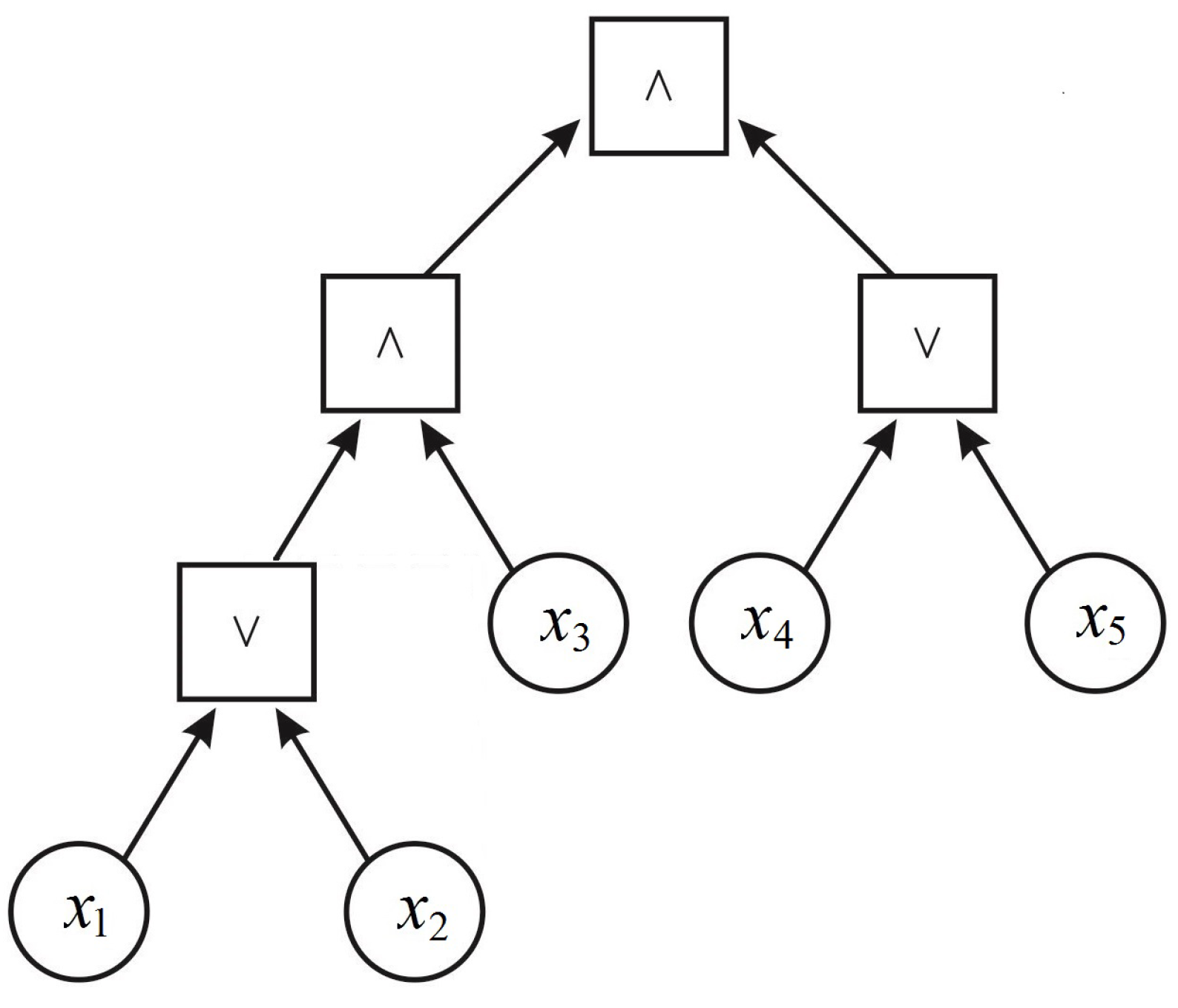
Suppose that the system consists of n elements, the state of which is determined by boolean variables $x_k,k=1,\dots ,n.$ If $x_k=1,$ then element k is in a working state, otherwise it fails. The state of an entire system is determined by a boolean function $A(x_1,\dots ,x_n),$ where independent random variables $x_k$ satisfies the condition $P(x_k=1)=p_k,k=1,\dots ,n.$ Then, the reliability of the system is determined by the expression $P(A(x_1,\dots ,x_n)=1).$

Boolean function A satisfies the natural monotonicity condition consequently [12] it belongs to the following recursively defined class of boolean functions $\mathcal{A}:$

$$x_k\in \mathcal{A},k=1,\dots ,n;A_1,A_2\in \mathcal{A}\Rightarrow A_1\vee A_2\in \mathcal{A},A_1\wedge A_2\in \mathcal{A}.$$

Let us now define a class of boolean functions, that characterize systems according to the modular principle, by a recursively definable class of boolean functions ${\mathcal{A}}_{\ast }\subset \mathcal{A}:$

$$x_k\in {\mathcal{A}}_{\ast },k=1,\dots ,n;A_1(x_k:k\in K_1),A_2(x_k:k\in K_2)\in {\mathcal{A}}_{\ast },$$

$$\mathrm{with}{K}_1,K_2\subseteq \{1,\dots ,n\},K_1\cap K_2=\varnothing \Rightarrow A_1\vee A_2\in {\mathcal{A}}_{\ast },A_1\wedge A_2\in {\mathcal{A}}_{\ast }.$$

So, boolean function $A(x_1,\dots ,x_n)\in {\mathcal{A}}_{\ast }$ may be depicted as in Figure 1.

From the definition of the class ${\mathcal{A}}_{\ast },$ the equalities follow

$$P(A_1\vee A_2=1)=P(A_1=1)+P(A_2=1)-P(A_1=1)P(A_2=1),$$

$$P(A_1\wedge A_2=1)=P(A_1=1)P(A_2=1).$$

Using these formulae, it is possible to calculate $P(A(x_1,\dots ,x_n)=1)$ in n steps as reliabilities of parallel and/or serial connections of two-poles.

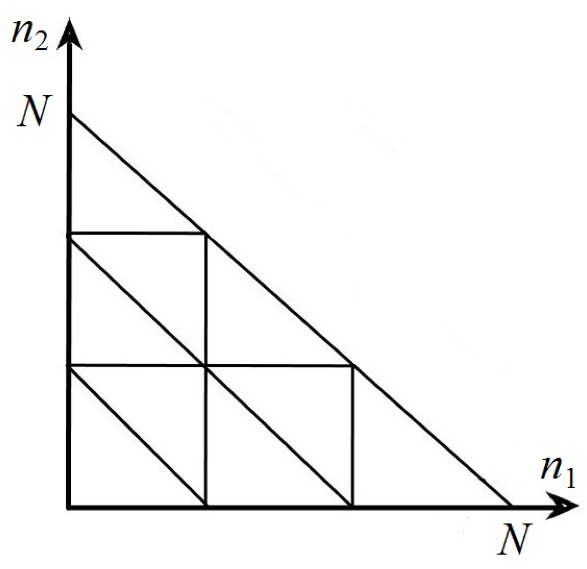
3. Disconnection Probability of Planar Graph with High Reliable Edges

The next model of reliability theory based on graph-theoretic representation consists of obtaining an asymptotic formula for the probability of incoherence of a planar graph with highly reliable edges. Assume that S is an undirected connected planar graph. It means that the graph S is placed on the plane and its edges do not intersect in internal points. Suppose that the graph S edges are highly reliable and fail independently with the probability $h\to 0.$ A cut of the graph S consists of edges whose deletion causes the graph to become disconnected. Further, we consider only cuts with minimal length (number of edges).

Calculate an asymptotic of a disconnection probability $P_h$ for such graph. From the Burtin–Pittel formula (see, for example [24]) we have:

$$P_h\sim c_m{h}^m,h\to 0,$$

(1)

where m is (minimal) cut length and $c_m$ is the number of cuts with length $m.$ In [13], it is proved that there is one-to-one correspondence between all cuts (with minimal length) in planar graph and all cycles with minimal length in dual graph $S^{\ast }.$

Let us denote $m^{\ast }$ the minimum vertices degree in $S,$ then $m\le m^{\ast }$ and from Euler’s formula [13] we have $m^{\ast }\le 5,$ where an equality may be reached.

Since we are interested in cuts with minimal length and, therefore, dual cycles with minimal length, then we shall limit ourselves to enumerating simple (without self-intersections) cycles of length $2,3,4,5$ in the dual graph. Denote $a_{ij}$ a number of edges contained in the intersection of the faces $z_i\cap z_j,i\ne j,a_{ii}=0,$ in the planar graph $S.$

Elements of l-th degree $A^l,l>1,$ of the matrix A are denoted by $a_{ij}^{\left(l\right)}.$ Using well-known formulas of the graph theory [25] we can calculate the number $c_k$ of simple cycles of length $k,k=2,3,4,5$ in the dual graph:

$$c_2=\frac{1}{4}\sum _{1\le i,j\le n}{a}_{ij}(a_{ij}-1),c_3=\frac{1}{6}tr{A}^3,c_4=\frac{1}{8}\left(tr{A}^4-2m-2\sum _{1\le i\ne j\le n}{a}_{ij}^{\left(2\right)}\right),$$

$$c_5=\frac{1}{10}\left(tr{A}^5-5tr{A}^3-5\sum _{i=1}^n\left(\sum _{j=1}^n{a}_{ij}-2\right)a_{ii}^{\left(3\right)}\right).$$

Then, the following equalities are valid: $m=min(k:2\le k\le 5:c_k>0).$

It follows from these formulas that the algorithm defined by them for calculating the asymptotic constants $m,c_m$ in the case of a planar graph has a complexity of no more than cubic. In the examples below, it is easy to see that this complexity can be significantly reduced. It should be noted that it is possible not only to calculate the constants $m,c_m$, but also to list the cycles of the minimum length in the graph $S^{\ast }$ and the corresponding sections interpreted by them as the bottlenecks of the graph S using computer algebra algorithms (see, for example [26]). It is worthwhile to note that the idea of using dual variables is also widely used in deterministic optimization problems (see for example [27,28]). These results may be generalized for graphs laid on two-dimensional surfaces.

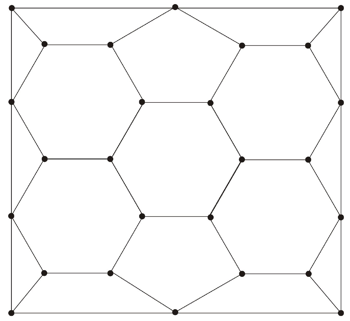
Numerical example. Consider the graph in Figure 2.

In this graph $m=3,c_3=22.$ The disconnection probability in this graph is calculated by the Monte-Carlo method with ${10}^6$ realizations (designated $P_{MC}$) and by asymptotic Formula (1) (designated $P_h$). Denote ${\Delta }_h=\frac{|P_{MC}-P_h|}{P_{MC}}.$ Obtained numerical results are represented in

Table 1. Results of $P_{MC},P_h,{\Delta }_h$ calculations.

h	${\mathit{P}}_{\mathit{MC}}$	${\mathit{P}}_{\mathit{h}}$	${\mathbf{\Delta }}_{\mathit{h}}$
0.01	0.000023	0.00002233	0.029
0.02	0.000179	0.000181	0.011

.

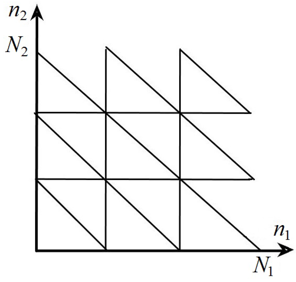
4. Construction and Calculation of Queuing Networks with Failures

However, graph-theoretic consideration is convenient to use not only in models of reliability theory. It turns out that it is possible to represent the classical Jackson network with various modifications caused by modern problems of the theory of communication and data transmission networks using original graph-theoretic considerations. This section discusses a queuing network with failures in nodes. Such a network arises in the mathematical theory of communications [14]. Assume that G is an open queuing network with m nodes (one-server or multi-server queuing systems), input intensity $\lambda >0,$ and route matrix

$${\displaystyle \Theta =\left|\right|{\theta }_{ij}{\left|\right|}_{k,i=0}^m:{\theta }_{k,k}=0;0<{\theta }_{ki}<1,k\ne i;\sum _{i=0}^m{\theta }_{ki}=1,0\le k\le m.}$$

Here, ${\theta }_{ki}$ is a probability of customer transition from ith node to jth node after its serving in ith node (0th node is an external source or external space). Then, the route matrix $\Theta$ satisfies the conditions

$$\forall i,j\in \{0,1,\dots ,m\}\exists i_1,i_2,\dots i_r\in \{1,\dots ,m\}:{\theta }_{i{i}_1}>0,{\theta }_{i_1{i}_2}>0,\dots {\theta }_{i_{r}j}>0,$$

and so the system of motion equations

$${\lambda }_k=\lambda {\theta }_{0k}+\sum _{j=1}^m{\lambda }_j{\theta }_{jk},k=1,\dots ,m,$$

has a unique solution with ${\lambda }_1>0,\dots ,{\lambda }_m>0.$

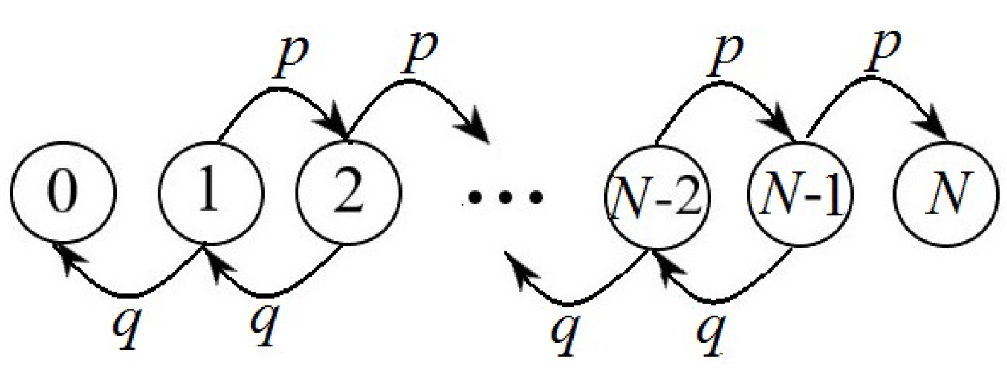
Suppose that kth node has $N_k$ servers with serving intensities ${\mu }_k,k=1,\dots ,m.$ Denote $n_k\left(t\right)$ a number of customers in kth node at moment $t.$ Then $(n_1\left(t\right),\dots ,n_m\left(t\right)),t\ge 0,$ is discrete Markov process, describing the network $G$.

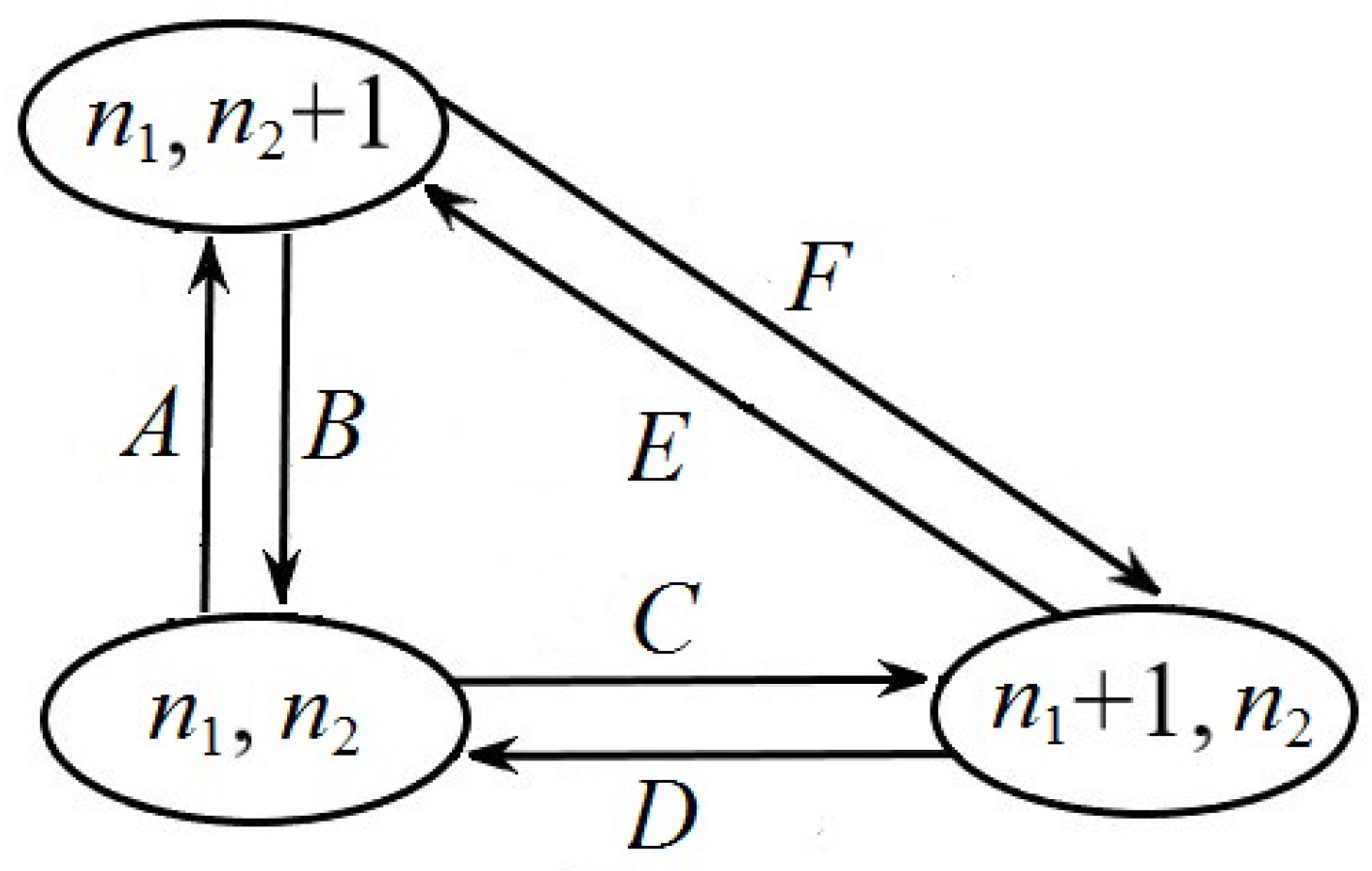
For simplicity and without limiting generality everywhere, we further assume $m=2.$ It is convenient to divide the construction of a weighted digraph of transition intensities on the set of states of a discrete Markov process $(n_1\left(t\right),n_2\left(t\right))$ into two stages. First, an undirected graph $\Gamma$ is constructed (Figure 3), consisting of triangular sub-graphs with vertices $(n_1,n_2),(n_1+1,n_2),(n_1,n_2+1).$

Then, each edge of such a triangular sub-graph is replaced by two oriented edges directed in opposite sides with corresponding transition intensities $A,B,C,D,E,F.$ The combination of these edges forms a triangular digraph $\Psi (n_1,n_2)$ (Figure 4).

Next, each undirected triangular sub-graph in $\Gamma$ should be replaced by the corresponding digraph of the form $\Psi (n_1,n_2).$ Here, the coefficients $A,C$ characterize the intensities of the arrivals of input customers to the network G nodes, the coefficients $B,D,E,F$ - the intensities of service at the nodes of the digraph $\Psi (n_1,n_2),$

$$A=\lambda {\theta }_{02},B={\mu }_2{n}_2{\theta }_{20},C=\lambda {\theta }_{01},D={\mu }_1{n}_1{\theta }_{10},E={\mu }_1{n}_1{\theta }_{12},F={\mu }_2{n}_2{\theta }_{21}.$$

(2)

Thus, digraph $\Psi (n_1,n_2)$ defines the network operation protocol, which includes permission or prohibition for certain transitions of customers. If edge $[(n_1,n_2),(n_1+1,n_2)]$ or edge $[(n_1,n_2),(n_1,n_2+1)]$ belong to the digraph $\Psi (n_1,n_2)$ then there is an allowance for input customer arrival to the first node or to the second node. If edge $[(n_1,n_2),(n_1-1,n_2)]$ or edge $[(n_1,n_2),(n_1,n_2-1)]$ belong to the digraph $\Psi (n_1,n_2)$ then there is an allowance for customer exit after service at the first node or at the second node from the network $G$. If these edges do not belong to the digraph $\Psi (n_1,n_2)$ then appropriate transitions are prohibited.

In these conditions, the Markov process $(n_1\left(t\right),n_2\left(t\right)),$ describing network $G$, is ergodic [15,29] and its limit distribution $P(n_1,n_2)$ satisfies stationary Kolmogorov–Chapman equations. We are looking for limit distribution of the Markov process $(n_1\left(t\right),n_2\left(t\right))$ in form ${\displaystyle P(n_1,n_2)=H\prod _{k=1}^2\frac{{\rho }_k^{n_k}}{n_k!},{\rho }_k={\lambda }_k/{\mu }_k,k=1,2.}$ The following equations follow from Formula (2)

$$\begin{gathered} P(n_1,n_2)(A+C)=P(n_1,n_2+1)B+P(n_1+1,n_2)D, \\ P(n_1,n_2+1)(B+F)=P(n_1,n_2)A+P(n_1+1,n_2)E, \\ P(n_1+1,n_2)(D+E)=P(n_1,n_2)C+P(n_1,n_2+1)F. \end{gathered}$$

(3)

Thus, the Markov process $(n_1\left(t\right),n_2\left(t\right))$ satisfies the stationary Kolmogorov–Chapman equations on the $\Psi (n_1,n_2)$ digraph. However, such different digraphs have not common edges, which means that the distribution $P(n_1,n_2)$ in this form satisfies the stationary Kolmogorov–Chapman equations on the entire graph $\Gamma .$

It follows that the process $(n_1\left(t\right),n_2\left(t\right)),$ defined in the graph on Figure 2, also satisfies these equations. Thus, a model of a queuing network with failures is constructed that satisfies the product theorem. If $L(\Gamma )=\{(n_1,n_2):0\le n_k\le N_k,k=1,2\}\backslash (N_1,N_2)$, then the constant H is defined by the equality

$$H={\left[\sum _{(n_1,n_2)\in L(\Gamma )}\prod _{k=1}^2\frac{{\rho }_k^{n_k}}{n_k!}\right]}^{-1}={\left[\prod _{k=1}^2\sum _{n_k=0}^{N_k}\frac{{\rho }_k^{n_k}}{n_k!}-\prod _{k=1}^2\frac{{\rho }_k^{N_k}}{N_k!}\right]}^{-1}.$$

We list possible generalizations of this construction. First, we can consider an open network with m nodes and failures. Then, an elementary sub graph $\Psi$ is a complete digraph containing a vertex $(n_1,\dots ,n_m)$ and vertices $(n_1+1,\dots ,n_m),(n_1,n_2+1,\dots ,n_m)\dots ,(n_1,\dots ,n_{m-1},n_m+1);n_k<N_k,k=1,\dots ,m,$ and limit distribution ${\displaystyle P(n_1,\dots ,n_m)=H\prod _{k=1}^m\frac{{\rho }_k^{n_k}}{n_k!}}$ satisfies stationary Kolmogorov–Chapman equations (m-dimensional analogue of Formula (3)).

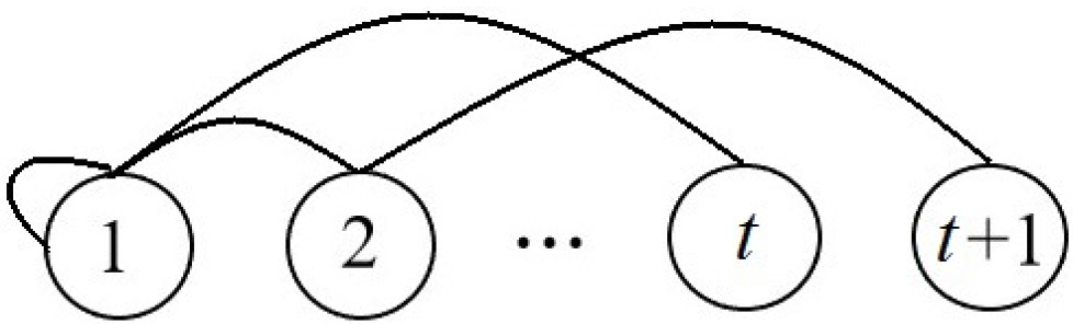
Another generalization is the change in the puncture of the network functioning in accordance with the change of the graph $\Gamma$ as follows (Figure 5) with $N\le min(N_1,N_2).$

We shall not discuss closed queuing networks in detail and only note that for them a connected graph $\Gamma$ is constructed from complete digraphs $\Psi$ with vertices $(n_1+1,n_2,\dots ,n_m),(n_1,n_2+1,n_3,\dots ,n_m),\dots ,(n_1,n_2,\dots ,n_{m-1},n_m+1).$

5. Limit Distribution in Queuing System $M\left|M\right|1|\infty$ with Randomly Varying Intensity of Input Flow

The graph-theoretic approach used in the previous section can be extended to the calculation of stationary distributions in queuing systems located in a random environment. Moreover, this approach allows us to identify new problems in which the stationary distribution does not obey the ergodicity hypothesis and to calculate the dependence of the stationary distribution on the initial state of the external environment. A large number of papers are devoted to queuing models with randomly varying parameters (see, for example [30,31]) with limit distributions, which do not depend on the initial state. However, there are models in which a random process, determining the parameters, develops on a segment with absorbing ends.

Consider queuing system $M\left|M\right|1|\infty$ with a service intensity $\mu$ and the intensity of the input flow $\lambda \left(t\right)=\Lambda \left(z\right(t\left)\right)>0,t\ge 0.$ Here $z\left(t\right)$ is defined by Markov chain $z_k,k=0,1,\dots ,$ describing a game to ruin the player [17], with the states $\{0,\dots ,N\},$ and $z\left(t\right)=z_k,k\le t<k+1,k=0,1,\dots$ The process $\lambda \left(t\right)=\Lambda \left(z\right(t\left)\right)>0,t\ge 0,$ with the states $\{\Lambda (0),\dots ,\Lambda (N\left)\right\}$ is Markov. Denote such queuing system by $\mathbf{M}.$

Markov chain $z_k,k=0,1,\dots ,$ has matrix $\Theta =\left|\right|{\theta }_{i,j}{\left|\right|}_{i,j=0}^N$ with non-zero transition probabilities (Figure 6).

$${\theta }_{i,i+1}=p,{\theta }_{i,i-1}=q,i=1,\dots ,N-1,{\theta }_{0,0}={\theta }_{N,N}=1,0<p<1,q=1-p.$$

If p is win probability and $q=1-p$ then ruin probability ${\Psi }_{z_0}\left(0\right)$ satisfies the system

$${\Psi }_{z_0}\left(0\right)=p{\Psi }_{z_0-1}\left(0\right)+q{\Psi }_{z_0+1}\left(0\right),z_0=2,\dots ,N-2,{\Psi }_0\left(0\right)=1,{\Psi }_N\left(0\right)=0.$$

with the solutions ([17] ch. I, § 9),

$${\Psi }_{z_0}\left(0\right)=\frac{{(p/q)}^{z_0}-{(p/q)}^N}{1-{(p/q)}^N},p\ne q;{\Psi }_{z_0}\left(0\right)=1-\frac{z_0}{N},p=q;z_0=0,\dots ,N,$$

(4)

and the winning probability ${\Psi }_{z_0}\left(N\right)=1-{\Psi }_{z_0}\left(0\right).$ Solution of the system (4) is the simplest discrete analogue of the Dirichlet problem ([16], ch. II, §§ 2–7).

So, the Markov chain $z_k,k\ge 0$ (and consequently the Markov process $z\left(t\right),t\ge 0$) has two-points limit distribution $({\Psi }_{z_0}\left(0\right),{\Psi }_{z_0}\left(N\right))$ ([17], ch. I, § 9)). Then, the input intensity $\lambda \left(t\right)$ has limit distribution

$$\underset{t\to \infty }{lim}P(\lambda \left(t\right)\equiv \Lambda \left(0\right))={\Psi }_{z_0}\left(0\right),\underset{t\to \infty }{lim}P(\lambda \left(t\right)\equiv \Lambda \left(N\right))={\Psi }_{z_0}\left(N\right).$$

In the queuing system $M\left|M\right|1|\infty$ with $\lambda \left(t\right)\equiv \lambda$ limit distribution of customers numbers

$$p\left(k\right)=(1-\rho ){\rho }^k,k=0,1,\dots ,\rho =\frac{\lambda }{\mu }<1.$$

Assume that $\Lambda \left(0\right),\dots ,\Lambda \left(N\right)<\mu$ and denote ${\displaystyle \rho \left(0\right)=\frac{\Lambda \left(0\right)}{\mu }<1,\rho \left(N\right)=\frac{\Lambda \left(N\right)}{\mu }<1.}$ It is not difficult to obtain that limit distribution $P_{z_0}\left(k\right),k=0,1,\dots ,$ of customers numbers $k\left(t\right)$ in the system $\mathbf{M}$ satisfies the equality, depending on initial state $z_0$

$$P_{z_0}\left(k\right)={\Psi }_{z_0}\left(0\right)(1-\rho \left(0\right)){\rho }^k\left(0\right)+{\Psi }_{z_0}\left(N\right)(1-\rho \left(N\right)){\rho }^k\left(N\right),k=0,1,\dots$$

So, the Markov process $(\lambda (t),k(t\left)\right)$ is not ergodic. These results may be spread onto multi-server systems with and without failures, on systems in which input to service intensities are randomly varying.

6. Convergence to the Limit Distribution in the Barabasi-Albert Model of a Growing Random Network

This section considers a random growing network. It cannot be attributed either to models of reliability theory or to queuing models. It is of an intermediate nature, because it is used in the description of the Internet and, therefore, is close to the theory of queuing. On the other hand, purely mathematically, this network is close to the problems of reliability theory and has analogues with systems built on the modular principle.

The main purpose of this section is to estimate the rate of convergence to limit distributions in the Barabashi–Albert model of growing random network (Figure 7) [7].

Let us consider the growing random network [7], in which a newly appearing vertex connects to any of the already existing vertices with a probability proportional to the degree of this vertex. At the initial step $t=1$, there is a single vertex and a loop associated with it. At the step $t\ge 1,$ we can determine the degree k of the vertex $s,$ equal to the number of incident edges.

Denote $p(k,s,t)$ the probability that at step $t\ge 1,k$ edges of an undirected network graph are connected to the vertex $s.$ Formally, we can define $p(k,s,t)=0,s>t,$ and so the following relations are obtained in [18]:

$$p(k,t,t)={\delta }_{k1},p(k,s,t+1)=\frac{k-1}{2t}p(k-1,s,t)+\left(1-\frac{k}{2t}\right)p(k,s,t),k\ge 1,$$

(5)

denote

$$P(k,t)=\frac{1}{t}\sum _{s=1}^{t}p(k,s,t).$$

(6)

Denote ${\prod }_{t+1}^t=1,$ from Formula (6) it is not difficult to obtain for $t\ge 1$

$$(t+1)P(k,t+1)=\frac{k-1}{2}P(k-1,t)+\left(t-\frac{k}{2}\right)P(k,t),k>1,$$

$$P(1,1)=1,P(k,t)=0,k>t\ge 1,P(0,t)\equiv 0,t\ge 1.$$

From here, it is not difficult to obtain

$$P(1,t+1)=\frac{1}{t+1}\left[1+\sum _{j=1}^t\prod _{s=j}^t\left(1-\frac{1}{2s}\right)\right],$$

(7)

$$P(k,t+1)=\frac{k-1}{2(t+1)}\sum _{j=1}^{t}P(k-1,j)\prod _{s=j+1}^t\left(1-\frac{k}{2s}\right),k\ge 2.$$

(8)

Remark 1.

In the future, we shall need to understand the expression ${\displaystyle \frac{\Gamma (1-A+t)}{\Gamma (-1-A)},}$ as ${\displaystyle \underset{\delta \to +0}{lim}\frac{\Gamma (1-A+t-\delta )}{\Gamma (-1-A-\delta )},}$ if $A,t$ are natural numbers. Here $\Gamma \left(z\right)$ is a gamma function.

Lemma 1.

For $A>0$, the equalities are valid

$$\sum _{j=1}^t\prod _{s=j}^t\left(1-\frac{A}{s}\right)=\frac{t-A}{1+A}+\frac{V\left(t\right)}{{(1+A)}^2\Gamma (-1-A)},V\left(t\right)=\frac{\Gamma (1-A+t)}{\Gamma (t+1)},$$

(9)

$$\sum _{j=1}^t\prod _{s=j+1}^t\left(1-\frac{A}{s}\right)=\frac{t+1}{1+A}+\frac{V\left(t\right)}{(1+A)\Gamma (1-A)}.$$

(10)

Proof. 

First, let $A>0$ not be a natural number. Denote ${\displaystyle S\left(t\right)=\sum _{j=1}^t\prod _{s=j}^t\left(1-\frac{A}{s}\right),}$ then

$$S\left(1\right)=1-A=\frac{1}{1+A}+\frac{V\left(1\right)}{{(1+A)}^2\Gamma (-1-A)},$$

hence, the Formula (9) if $t=1$ is proved.

Suppose that this formula is true for a given $t>1,$ we prove it for $t+1:$

$$S(t+1)=\sum _{j=1}^{t+1}\prod _{s=j}^{t+1}\left(1-\frac{A}{s}\right)=\frac{t+1-A}{t+1}(S\left(t\right)+1)$$

$$=\frac{t+1-A}{t+1}\left(\frac{t-A}{1+A}+\frac{V\left(t\right)}{{(1+A)}^2\Gamma (-1-A)}\right)=\frac{t+1-A}{t+1}+\frac{V(t+1)}{{(1+A)}^2\Gamma (-1-A)}.$$

So, the relation (9) is true for all natural $t.$ The relation (10) may be proved similarly. For natural A, the function $V\left(t\right)$ in Formulas (9) and (10) is understood in the sense that remark 2 contains. □

Denote

$$f_k\left(t\right)=P(k,t+1)-\Pi \left(k\right),\Pi \left(k\right)=\frac{4}{k(k+1)(k+2)},(k\ge 1),$$

(11)

where $P(k,t)\to \Pi \left(k\right),k\ge 1,t\to \infty .$

Theorem 1.

At $k\ge 1$ the relation is fulfilled

$$f_k\left(t\right)\sim \frac{t^{-3/2}}{3\sqrt{\pi }},t\to \infty .$$

(12)

Proof. 

For $A>0$ it is possible to obtain from Stirling’s formula:

$$V\left(t\right)=\frac{\Gamma (1-A+t)}{\Gamma (t+1)}\sim t^{-A},(t\to \infty ).$$

(13)

Indeed, it is well known ([32], Chapter 1) that $\Gamma (1+t)\sim t^t{e}^{-t}\sqrt{2\pi t},t\to \infty ,$ so

$$\frac{\Gamma (1+t-A)}{\Gamma \left(t\right)}\sim \frac{{(t-A)}^{t-A}{e}^{-(t-A)}\sqrt{2\pi (t-A)}}{t^t{e}^{-t}\sqrt{2\pi t}}\sim \frac{t^{t-A}{(1-A/t)}^{t-A}{e}^A}{t^t}$$

$$=t^{-A}{e}^A{(1-A/t)}^{At/A}{(1-A/t)}^{-A}\sim t^{-A}{e}^A{e}^{-A}\sim t^{-A},t\to \infty .$$

Let $k=1,$ then the relation (12) follows from Formulas (7), (9) and (13) when $A=1/2:$

$$f_1\left(t\right)=P(1,t+1)-\Pi \left(1\right)=\frac{1}{t+1}\left(1+\frac{t-1/2}{3/2}+\frac{V\left(t\right)}{{(3/2)}^2\Gamma (-3/2)}\right)-\frac{2}{3}$$

$$\sim \frac{4t^{-1/2}}{9\Gamma (-3t/2)}=\frac{t^{-3/2}}{3\sqrt{\pi }},t\to \infty .$$

Let us assume that the relation (12) holds for $k-1>0,$ and prove its validity for $k.$ We look for $f_k\left(t\right)$ in the form $f_k\left(t\right)=a_k\left(t\right)+b_k\left(t\right),$ where

$$a_k\left(t\right)=\frac{k-1}{2(t+1)}\sum _{j=1}^t\Pi (k-1)\prod _{s=j+1}^t\left(1-\frac{k}{2s}\right)-\Pi \left(k\right),$$

$$b_k\left(t\right)=\frac{k-1}{2(t+1)}\sum _{j=1}^t{f}_{k-1}(j-1)\prod _{s=j+1}^t\left(1-\frac{k}{2s}\right).$$

Therefore, by virtue of Formulas (10) and (11) for $A=k/2$

$$a_k\left(t\right)=\frac{4}{k(k+1)}\left[\frac{1}{2(t+1)}\sum _{j=1}^t\prod _{s=j+1}^t\left(1-\frac{k}{2s}\right)-\frac{1}{k+2}\right]$$

$$=\frac{4}{k(k+1)}\left[\frac{1}{2(t+1)}\left(\frac{t+1}{1+k/2}+\frac{V\left(t\right)}{(1+k/2)\Gamma (1-k/2)}\right)-\frac{1}{k+2}\right]$$

$$=\frac{4V\left(t\right)}{2(t+1)k(k+1)(1+k/2)\Gamma (1-k/2)}\sim \frac{\Pi \left(k\right)t^{-1-k/2}}{\Gamma (1-k/2)}=o\left(t^{-3/2}\right),(t\to \infty ).$$

In turn, by the assumption of induction ${\displaystyle f_{k-1}\left(t\right)\sim \frac{t^{-3/2}}{3\sqrt{\pi }},t\to \infty ,}$ properties of the gamma function and Formula (13) for $A=k/2$ we have

$$b_k\left(t\right)=\frac{k-1}{2(t+1)}\sum _{j=1}^t{f}_{k-1}(j-1)\frac{V\left(t\right)}{V\left(j\right)}\sim \frac{k-1}{2(t+1)}{\int }_1^t\frac{x^{k/2}}{3\sqrt{\pi }{x}^{3/2}{t}^{k/2}}dx\sim \frac{t^{-3/2}}{3\sqrt{\pi }},(t\to \infty ).$$

Hence the validity of the asymptotic relation (12) follows for an arbitrary $k$. □

Let us consider a model of Dorogovtsev’s growing network, in which an edge from a newly appearing vertex to existing vertices has a probability proportional to the degree of this vertex plus $a.$ Here, $a>0$ is a parameter of the model. In [18], the following relations are obtained:

$$p(k,s,t+1)=\frac{k-1}{t(1+a)}p(k-1,s,t)+\left(1-\frac{k+a}{t(1+a)}\right)p(k,s,t),p(k,t,t)={\delta }_{k0},k\ge 0.$$

From Formula (6), we have

$$P(k,t+1)=\frac{1}{t(a+1)}\left[P(k,t)((a+1)(t-1)-k-a)+P(k-1,t)(k-1+a)+(1+a){\delta }_{k0}\right],$$

$$P(0,1)=1,P(k,t)=0,k\ge t,P(-1,t)\equiv 0,t\ge 0$$

By analogy with (7) and (8) it is not difficult to obtain

$$P(0,t+1)=\frac{1}{t}\left[1-\frac{a}{a+1}\prod _{l=1}^{t-1}\left(1-\frac{a}{l(a+1)}\right)+\sum _{s=1}^{t-1}\prod _{j=s}^{t-1}\left(1-\frac{a}{j(a+1)}\right)\right],$$

(14)

$$P(k,t+1)=\frac{k-1+a}{t(a+1)}\sum _{s=1}^{t}P(k-1,s)\prod _{j=s}^{t-1}\left(1-\frac{k+a}{(a+1)j}\right),k>0.$$

(15)

Denote $A_k=(k+a)/(a+1),k\ge 0,$

$$\Pi \left(k\right)=(1+a)\frac{\Gamma (1+2a)\Gamma (k+a)}{\Gamma \left(a\right)\Gamma (k+2+2a)},f_k\left(t\right)=P(k,t+1)-\Pi \left(k\right),k\ge 0.$$

Theorem 2.

The following relations are fulfilled

$$f_k\left(t\right)\sim C_k{t}^{-1-A_0},t\to \infty ,k\ge 0,$$

$$C_0=\frac{1}{{(1+A_0)}^2\Gamma (-1-A_0)}-\frac{A_0}{\Gamma (1-A_0)},\frac{C_{k-1}(k-1+a)}{(a+1)(A_k-A_0)}=C_k,k>0.$$

(16)

Proof. 

By virtue of Formulas (9), (13) and (14) for $A=A_0$ we have

$$f_0\left(t\right)=P(0,t+1)-\Pi \left(0\right)=\frac{1}{t}\left[1-\frac{A_0\Psi (t-1)}{\Gamma (1-A_0)}+\frac{t-(1+A_0)}{1+A_0}+\frac{\Psi (t-1)}{\Gamma (-1-A_0){(1+A_0)}^2}\right]$$

$$-\frac{1+a}{1+2a}=\frac{\Psi (t-1)C_0}{t}\sim C_0{t}^{-1-A_0},t\to \infty .$$

For $k>0$, we are looking for $f_k\left(t\right)=P(k,t+1)-\Pi \left(k\right)$ in the form $f_k\left(t\right)=a_k\left(t\right)+b_k\left(t\right),$

$$a_k\left(t\right)=\frac{k-1+a}{t(a+1)}\sum _{s=1}^t\Pi (k-1)\prod _{j=s}^{t-1}\left(1-\frac{A_k}{j}\right)-\Pi \left(k\right),$$

$$b_k\left(t\right)=\frac{k-1+a}{t(a+1)}\sum _{s=1}^t{f}_{k-1}(s-1)\prod _{j=s}^{t-1}\left(1-\frac{A_k}{j}\right).$$

Then, by virtue of Formula (13) for $t\to \infty$ and $A=A_k$ we have

$$a_k\left(t\right)=\frac{(k-1+a)\Pi (k-1)}{t(a+1)}\left[\sum _{s=1}^{t-1}\prod _{j=s}^{t-1}\left(1-\frac{A_k}{j}\right)+1\right]-\Pi \left(k\right)$$

$$=\frac{(k-1+a)\Pi (k-1)\Psi (t-1)}{t(a+1)\Gamma (-1-A_k){(1+A_k)}^2}\sim \frac{(k-1+a)\Pi (k-1)t^{-A_k-1}}{{(1+A_k)}^2(a+1)\Gamma (-1-A_k)}.$$

In turn, from the assumption of induction $f_{k-1}\left(t\right)\sim C_{k-1}{t}^{-1-A_0}$, by virtue of the relation $A_k>A_0$ and Formula (13) for $A=A_k$, we have

$$b_k\left(t\right)=\frac{k-1+a}{t(a+1)}\sum _{s=1}^t{f}_{k-1}(s-1)\prod _{j=s}^{t-1}\left(1-\frac{A_k}{j}\right)=\frac{k-1+a}{t(a+1)}\sum _{s=1}^t{f}_{k-1}(s-1)\frac{\Psi (t-1)}{\Psi (s-1)}$$

$$\sim \frac{C_{k-1}(k-1+a)}{t^{1+A_0}(a+1)(A_k-A_0)}=C_k{t}^{-1-A_0},t\to \infty .$$

Thus, the asymptotic relation (16) is proved for an arbitrary $k$. □

Remark 2.

Dorogovtsev’s model [18] is widely used in models of growing random networks. For small a, it gives sufficiently simple description of the Internet network, using a power distribution of the degree of network nodes

$$\Pi \left(k\right)\sim D{k}^{-2-a},D=\frac{(1+a)\Gamma (1+2a)}{\Gamma \left(a\right)},k\to \infty ,$$

in which its parameter is close to two [21].

Remark 3.

Similarly, an exponentially growing random network, in which the newly appearing vertex connects to any of the already existing vertices with equal probabilities, may also be studied.

7. Discussion

This paper presents the main examples known to the author of the use of random processes on graphs for modelling and analysing various modern computer science systems. At the same time, each of the above examples allows for different generalizations. However, these generalizations require a more detailed definition and research using both probabilistic methods and methods of graph theory.

In particular, models of systems built on the modular principle have just begun to penetrate into logical-probabilistic modelling [22]. Their application can expand the possibilities of this method of stochastic systems modelling. Models of reliability systems represented by planar graphs with highly reliable edges are built at the junction of reliability theory and planar graph theory. Such a study allows us to expand the possibilities of logical probabilistic modelling by introducing ideas from graph theory and topology [13] into it. The use of oriented graphs defining protocols in queuing networks makes it possible to obtain formulas for limit distributions in data transmission networks, in particular, describing networks of the latest generations [14]. The calculation of limit distributions in queuing systems placed in a random environment and not obeying the ergodicity hypothesis allows us to expand the capabilities of known methods [30,31] for performing such calculations. The asymptotic formulas of the difference between the prelimit and limit distributions in models of growing random networks are accurate. The asymptotic formulas of the difference between the limit and limit distributions in the models of growing random networks obtained in this paper are accurate. This allows us to strengthen the results of the papers [7,18].

8. Conclusions

The possibility of strengthening the known results on the theory of reliability, queuing and on the theory of growing random networks is presented. It seems to the author that the continuation of this research can become a source of new and significant results in the listed and already known areas of probabilistic modelling.