Stability Switches and Double Hopf Bifurcation Analysis on Two-Degree-of-Freedom Coupled Delay van der Pol Oscillator

Abstract

In this paper, the normal form and central manifold theories are used to discuss the influence of two-degree-of-freedom coupled van der Pol oscillators with time delay feedback. Compared with the single-degree-of-freedom time delay van der Pol oscillator, the system studied in this paper has richer dynamical behavior. The results obtained include: the change of time delay causing the stability switching of the system, and the greater the time delay, the more complicated the stability switching. Near the double Hopf bifurcation point, the system is simplified by using the normal form and central manifold theories. The system is divided into six regions with different dynamical properties. With the above results, for practical engineering problems, we can perform time delay feedback adjustment to make the system show amplitude death, limit loop, and so on. It is worth noting that because of the existence of unstable limit cycles in the system, the limit cycle cannot be obtained by numerical solution. Therefore, we derive the approximate analytical solution of the system and simulate the time history of the interaction between two frequencies in Region IV.

1. Introduction

The van der Pol oscillator is a limit cycle oscillation of vacuum tube amplifiers discovered by Dutch scientists. The limit cycle oscillation can be expressed by the following nonlinear differential equations:

$$\ddot{x}+x-\epsilon (1-x^2)\dot{x}=0.$$

(1)

The van der Pol oscillator exists in many aspects, such as image encryption [1] and signal detection [2]. It is worth noting that we can only solve the system by approximating analytical and numerical methods, including multiple time scales [3] and average methods [4]. Of course, in addition to the development of research methods, many scholars have studied the dynamic behavior of van der Pol oscillators under the influence of time delay [5,6] and non-smooth oscillators [7].

The coupling of oscillators usually generates many new phenomena, such as synchronization, phase locking, and amplitude death. Stankevich et al. [8] studied quasi-periodic bifurcations of five coupled van der Pol oscillators. Bukh and Anishchenko [9] studied the spiral wave, target wave, and chimeric wave in coupled van der Pol oscillators. Singh and Yadava [10] found transient chaos and stable chaotic dynamics in coupled autonomous van der Pol oscillations, but this is a rare case. Then they revealed that the nonlinear restoring forces in a pair of van der Pol oscillators can induce a transient chaotic route by a small disturbance to the amplitude of an oscillator. Algaba et al. [11] investigated canard explosion in van der Pol electronic oscillators. They developed a new effective program which can calculate the approximate value of critical parameters of any desired order. Qian and Fu [12] studied the primary resonance of van der Pol systems under parametric excitation by using the multi-scale method (MSM) and homotopy analysis method (HAM). It was found that the margin of error is too small, while Kumar and Varshney [13] proposed an effective perturbation algorithm for solving the van der Pol oscillator equation by combining the multi-scale method with the modified Lindstedt Poincare method.

Most of the above literature is based on coupled van der Pol oscillators without time delay. In this paper, we will use the method of normal form and center manifolds to study the two-degree-of-freedom (TDOF) time delay van der Pol system. For the method of center manifold and normal form, we can refer to the references [14,15]. Bifurcation analysis and branch solutions can refer to the literature [16,17]. In fact, we can also use the normal form theory and center manifold theory to analyze other bifurcation types, such as double Hopf [18,19] and Fold-Hopf [20,21]. Qian et al. [22] studied the dynamical behavior of double-Hopf bifurcations by the multi-scale method. Ge and Xu considered four neurons and two delays of the bidirectional associative memory (BAM) neural network. The dynamic behaviors in the neighborhood of the Fold-Hopf bifurcation point are classified qualitatively by using the normal form theory and center manifold theory [21]. Chen and Yu [18] studied the oscillator with time delay, in which the external excitation causes double Hopf bifurcation. They obtained the critical conditions for double Hopf bifurcation and approximate solutions of periodic and quasi-periodic motions. Based on the study of Guckenheimer [14], Du et al. [19] presented the calculation form of double Hopf bifurcation. Based on the normal form and center manifold theories, Song and Xu analyzed the complex dynamic bifurcation of double neural networks with time-delay coupling. The dynamic behaviors are classified, including stable equilibrium point, periodic solution, 2-torus, 3-torus, and chaotic motions [20]. They also found that multiple delays lead to a stable switch in the dynamic behavior of the system [23]. Besides, Song and Xu studied Fold-Hopf bifurcation in a neural network system composed of two delay coupled neural oscillators. It was found that the system exhibits different bursting behaviors with different time delays [24]. Song et al. also considered the fast-slow system with time delay and obtained the bursting oscillation of codimension two [25,26].

It can be seen that in the literature [8,9,10,11], we have studied the branching, chaos, canard explosion, and other phenomena of the coupled van der Pol oscillators without time delay from the phenomenology. However, they still lack the analysis of the theory behind the coupled van der Pol oscillators. Additionally, through the literature [17,20,23,24,25,26], we can get conclusions about the time delay nervous system. However, the above literature does not involve the study of coupled van der Pol oscillators with time delay feedback. Therefore, the research in this article is original. This research can also realize the change of system dynamics through the adjustment of time delay feedback, which can provide theoretical guidance for complex phenomena in engineering.

In this paper, we will use normal form theory and center manifold theory to study van der Pol oscillators with two degrees of freedom. Some of the data in the article were generated by the DDE_BIFTOOL package [27]. In Section 2, we discuss the Hopf bifurcation and stability switching of Equation (2.1); In Section 3, we analyze the stability of double Hopf bifurcation with two time delays, and divide the region near the double Hopf according to its dynamic characteristics. Then, a numerical simulation and approximate analytical solution are given.

2. Stability Analysis and Hopf Bifurcation

In this part, we discuss the stability and Hopf bifurcation of Equation (2) at the unique equilibrium $(0,0,0,0)$. Additionally, Equation (2) can be shown as below:

$$\begin{array}{cc}\hfill \dot{x}{}_1\left(t\right)=& x_2\left(t\right),\hfill \\ \hfill \dot{x}{}_2\left(t\right)=& k(1-x_1{\left(t\right)}^2)x_2\left(t\right)-l{x}_1\left(t\right)-({\beta }_1{x}_1(t-{\tau }_1)-{\beta }_2{x}_3(t-{\tau }_2))+tanh\left(x_1(t-{\tau }_1)x_3(t-{\tau }_2)\right),\hfill \\ \hfill \dot{x}{}_3\left(t\right)& =x_4\left(t\right),\hfill \\ \hfill \dot{x}{}_4\left(t\right)=& k(1-x_3{\left(t\right)}^2)x_4\left(t\right)-l{x}_3\left(t\right)-({\beta }_1{x}_3(t-{\tau }_1)-{\beta }_2{x}_1(t-{\tau }_2))+tanh\left(x_3(t-{\tau }_1)x_1(t-{\tau }_2)\right).\hfill \end{array}$$

(2)

The linear part of Equation (2) is as follows:

$$\begin{array}{cc}\hfill \dot{x}& {}_1\left(t\right)=x_2\left(t\right),\hfill \\ \hfill \dot{x}& {}_2\left(t\right)=k{x}_2\left(t\right)-l{x}_1\left(t\right)-({\beta }_1{x}_1(t-{\tau }_1)-{\beta }_2{x}_3(t-{\tau }_2)),\hfill \\ \hfill \dot{x}& {}_3\left(t\right)=x_4\left(t\right),\hfill \\ \hfill \dot{x}& {}_4\left(t\right)=k{x}_4\left(t\right)-l{x}_3\left(t\right)-({\beta }_1{x}_3(t-{\tau }_1)-{\beta }_2{x}_1(t-{\tau }_2)).\hfill \end{array}$$

(3)

The characteristic equation of the linearized System (3) reduces to

$$\begin{array}{c}({\lambda }^2-k\lambda +l+{\beta }_1{e}^{-\lambda {\tau }_1}-{\beta }_2{e}^{-\lambda {\tau }_2})({\lambda }^2-k\lambda +l+{\beta }_1{e}^{-\lambda {\tau }_1}+{\beta }_2{e}^{-\lambda {\tau }_2})=0.\hfill \end{array}$$

(4)

When ${\tau }_1={\tau }_2=0$, the characteristic equation becomes $({\lambda }^2-k\lambda +l+{\beta }_1-{\beta }_2)({\lambda }^2-k\lambda +l+{\beta }_1+{\beta }_2)=0$. If the characteristic equation has zero real part eigenvalues at the equilibrium point, then the equilibrium point is hyperbolic. The Hartman-Grobman theorem tells us that the orbit topology near the hyperbolic equilibrium point is equivalent to the linearized system.

We consider ${\lambda }^2-k\lambda +J_n=0,n\in \{1,2\}$, where

$$\begin{array}{c}{J}_1=l+{\beta }_1{e}^{-\lambda {\tau }_1}-{\beta }_2{e}^{-\lambda {\tau }_2},J_2=l+{\beta }_1{e}^{-\lambda {\tau }_1}+{\beta }_2{e}^{-\lambda {\tau }_2}.\hfill \end{array}$$

(5)

We can write the characteristic equation into the form of $({\lambda }^2-k\lambda +J_1)({\lambda }^2-k\lambda +J_2)=0$. Take $J_1$ as an example. Let $\pm i{\omega }_{01}({\omega }_{01}>0)$ be a pair of purely imaginary roots of Equation (4).

$$\begin{array}{c}{\left(i{\omega }_{01}\right)}^2-ki{\omega }_{01}+l+{\beta }_1{e}^{-i{\omega }_{01}{\tau }_1}-{\beta }_2{e}^{-i{\omega }_{01}{\tau }_2}=0.\hfill \end{array}$$

(6)

Segregating the real part and imaginary part of Equation (6), we get

$$\begin{array}{c}\hfill \left\{\begin{array}{c}-{\omega }_{01}^2+l+{\beta }_{1}cos\left({\omega }_{01}{\tau }_1\right)-{\beta }_{2}cos\left({\omega }_{01}{\tau }_2\right)=0,\hfill \\ k{\omega }_{01}+{\beta }_{1}sin\left({\omega }_{01}{\tau }_1\right)-{\beta }_{2}sin\left({\omega }_{01}{\tau }_2\right)=0.\hfill \end{array}\right.\end{array}$$

(7)

Eliminating ${\tau }_2$ from Equation (7), we obtain

$$\begin{array}{c}G({\omega }_{01},{\tau }_2)={(-{\omega }_{01}^2-{\beta }_{2}cos\left({\omega }_{01}{\tau }_2\right)+l)}^2+{(k{\omega }_{01}-{\beta }_{2}sin\left({\omega }_{01}{\tau }_2\right))}^2-{\beta }_1^2.\hfill \end{array}$$

(8)

Where there is fixed ${\tau }_2$, if $G({\omega }_{01},{\tau }_2)=0$ has one positive root, then there is a critical value $\tau$ determined by

$$\begin{array}{c}{\displaystyle {\tau }_{11}^j=\frac{1}{{\omega }_{01}}\left[arccos\frac{-{\omega }_{01}^2+l-{\beta }_{2}cos\left({\omega }_{01}{\tau }_2\right)}{-{\beta }_1}+2j\pi \right],j=0,1,2\cdots }\hfill \end{array}.$$

(9)

When the system passes through the critical value, it will lose stability. In order to make sure the Hopf bifurcation occurs, we also need to verify its transversality condition. Without loss of generality, here we calculate the derivative of $\lambda$ to ${\tau }_1$.

$$\begin{array}{c}{\displaystyle \frac{d\lambda }{d{\tau }_1}=\frac{\lambda {\beta }_1{e}^{-\lambda {\tau }_1}}{2\lambda -k-{\beta }_1{e}^{-\lambda {\tau }_1}{\tau }_1+{\beta }_2{e}^{-\lambda {\tau }_2}{\tau }_2}.}\hfill \end{array}$$

(10)

Notice that if ${\displaystyle \frac{d\lambda }{d{\tau }_1}\ne 0}$, then there is a Hopf bifurcation. Thus, we draw the following conclusion.

Theorem 1.

Considering Equation (2),

(i) When $G({\omega }_{01},{\tau }_2)=0$ has no positive real root, the trivial equilibrium of the system Equation (2) is asymptotically stable for any ${\tau }_1$.

(ii) When $G({\omega }_{01},{\tau }_2)=0$ has one positive root, there is a critical value ${\tau }_{11}$. The trivial equilibrium of system Equation (2) is asymptotically stable for ${\tau }_1\in (0,{\tau }_{11})$, and it will lose the stability for ${\tau }_1>{\tau }_{11}$, which means the system will undergo a Hopf bifurcation for ${\tau }_1={\tau }_{11}$.

(iii) When $G({\omega }_{01},{\tau }_2)=0$ has several pairs of positive real roots, there exist several critical values. Then we divide the interval, and we can also find that trivial equilibriums of systems are asymptotically stable on finite intervals.

For example, we choose $l=0.5,{\beta }_1=0.4,{\beta }_2=-0.4,k=-0.5$, where the roots of function G are related to $\omega$, and the figures of function G are displayed in Figure 1 for different ${\tau }_2$. Correspondingly, in Figure 2a and Figure 3a, we show the eigenvalue diagram of the system when ${\tau }_1$ changes. Figure 2b,c and Figure 3b show the real and imaginary parts of the eigenvalues when ${\tau }_1,{\tau }_2$ are fixed.

Figure 1. Roots of function G when $l=0.5,{\beta }_1=0.4,{\beta }_2=-0.4,k=-0.5$, (a) ${\tau }_2=1$, (b) ${\tau }_2=8$.

Figure 2. When ${\tau }_2=1$, (a) the eigenvalue diagrams of the system for ${\tau }_1$ kept changing, (b) shows the real and imaginary parts of eigenvalue diagrams of the system for ${\tau }_1=0.1$, and (c) shows the real and imaginary parts of eigenvalue diagrams of the system for ${\tau }_1=1$.

Figure 3. When ${\tau }_2=8$, (a) the eigenvalue diagram of the system for ${\tau }_1$ kept changing, and (b) shows the eigenvalue sketch diagram of the system for ${\tau }_1=1$.

When ${\tau }_2=1$, $G\left({\omega }_{01}\right)=0$ has two positive real roots, it means there will be an interval which makes the system stable. If ${\tau }_1$ separates from this interval, the stability of the system will change and the positive real part will appear, which can be observed in Figure 2a. When ${\tau }_1$ increases, the blue curve obviously crosses the zero line, then the blue curve falls from above the zero line. When ${\tau }_2=8$, the situation becomes more complicated. $G\left({\omega }_{01}\right)=0$ has several positive real roots, and the stability switching of the system will be more frequent. It can be seen from Figure 3a that multiple curves of the system move back and forth on the zero line, and it illustrates the complexity of positive real characteristic roots.

In order to explain the stability switching of the system more clearly. We take ${\tau }_2=1,{\tau }_1=0.1,1$ and ${\tau }_2=8,{\tau }_1=1$, respectively. Comparing Figure 2b,c with Figure 3b, it is found that time delay can certainly make the system go from stable to unstable.

3. Analysis of Double Hopf Bifurcation

In this part, we will study the nature of double Hopf bifurcation about the direction and the stability of bifurcating periodic solutions with two time delays, ${\tau }_1$ and ${\tau }_2$. Firstly, we study double Hopf bifurcation based on the normal form theory and center manifold theorem. Secondly, we carry out the numerical simulations.

3.1. Computation of Normal Form and Center-Manifold Reduction

For convenience, let $\beta ={\beta }_1=-{\beta }_2$; then we derive the unfolding of the System (2) by the normal form theory and center manifold theorem, and then we are able to reach the stability near the critical value. Now, we need to regulate the time delay by changing the time. Let ${\displaystyle t\mapsto \frac{t}{{\tau }_1}}$ and ${\displaystyle r=\frac{{\tau }_2}{{\tau }_1}}$, where the system becomes:

$$\begin{array}{c}{\dot{x}}_1\left(t\right)={\tau }_1{x}_2\left(t\right),\hfill \\ {\dot{x}}_2\left(t\right)={\tau }_1[k(1-x_1{\left(t\right)}^2)x_2\left(t\right)-l{x}_1\left(t\right)-\beta (x_1(t-1)+x_3(t-r))+tanh\left(x_1(t-1)x_3(t-r)\right)],\hfill \\ {\dot{x}}_3\left(t\right)={\tau }_1{x}_4\left(t\right),\hfill \\ {\dot{x}}_4\left(t\right)={\tau }_1[k(1-x_3{\left(t\right)}^2)x_4\left(t\right)-l{x}_3\left(t\right)-\beta (x_1(t-r)+x_3(t-1))+tanh\left(x_1(t-r)x_3(t-1)\right)].\hfill \end{array}$$

(11)

Regarding the time delays ${\tau }_1$ and r as bifurcation parameters, we set

$$\begin{array}{c}{\tau }_1={\tau }_1^c+\epsilon {\delta }_1,r=r^c+\epsilon {\delta }_2,\hfill \end{array}$$

(12)

where $\epsilon {\delta }_1$ and $\epsilon {\delta }_2$ are unfolding parameters. It follows that

$$\begin{array}{c}{\tau }_2={\tau }_{1}r={\tau }_2^c+\epsilon (r^c{\delta }_1+{\tau }_1^c{\delta }_2)+o\left(\epsilon \right).\hfill \end{array}$$

(13)

We rewrite the system as follows:

$$\begin{array}{c}{\dot{x}}_1\left(t\right)=({\tau }_1^c+\epsilon {\delta }_1)x_2\left(t\right),\hfill \\ {\dot{x}}_2\left(t\right)=({\tau }_1^c+\epsilon {\delta }_1)[k(1-x_1{\left(t\right)}^2)x_2\left(t\right)-l{x}_1\left(t\right)-\beta (x_1(t-1)+x_3(t-r^c-\epsilon {\delta }_2))\hfill \\ +tanh\left(x_1(t-1)x_3(t-r^c-\epsilon {\delta }_2)\right)],\hfill \\ {\dot{x}}_3\left(t\right)=({\tau }_1^c+\epsilon {\delta }_1)x_4\left(t\right),\hfill \\ {\dot{x}}_4\left(t\right)=({\tau }_1^c+\epsilon {\delta }_1)[k(1-x_3{\left(t\right)}^2)x_4\left(t\right)-l{x}_3\left(t\right)-\beta (x_1(t-r^c-\epsilon {\delta }_2)+x_3(t-1))\hfill \\ +tanh\left(x_3(t-1)x_1(t-r^c-\epsilon {\delta }_2)\right)].\hfill \end{array}$$

(14)

To apply the central manifold reduction, we need to rewrite it into functional differential form. $C([-\tau ,0],R^4)$ is the Banach space of continuous functions, where $\tau =max\{1,r\}$. For any $\varphi \in C$, we define:

$$\begin{array}{c}\eta (\theta ,\epsilon )=({\tau }_1^c+\epsilon {\delta }_1)A_1\delta \left(\theta \right)-({\tau }_1^c+\epsilon {\delta }_1)A_2\delta (\theta +1)-({\tau }_1^c+\epsilon {\delta }_1)A_3\delta (\theta +r^c+\epsilon {\delta }_2).\hfill \end{array}$$

(15)

Then we can obtain $L_{\epsilon }\varphi \left(\theta \right),A\left(\epsilon \right)\varphi \left(\theta \right),R\left(\epsilon \right)\varphi \left(\theta \right),A^{*}\left(\epsilon \right)\psi \left(s\right)$, and the bilinear inner product. (The detailed process is in the Appendix A).

If System (11) has two pairs of purely imaginary eigenvalues $\Lambda =\{\pm i{\omega }_{01},\pm i{\omega }_{02}\}$ and other eigenvalues are negative, the phase space C can be divided into two subspaces. That is, $C=P_{\Lambda }\oplus Q_{\Lambda }$. $P_{\Lambda }$ is the central subspace obtained by extending the basis vector of linear operator $A_{\epsilon }$ with respect to $\pm i{\omega }_{01},\pm i{\omega }_{02}$. $Q_{\Lambda }$ is its complementary space.

We suppose ${\varphi }_j\left(\theta \right)$ and ${\psi }_j\left(s\right)$ are the eigenvectors of $A\left(0\right)$ and $A^{*}\left(0\right)$. They correspond to eigenvalue $i{\omega }_{0j},-i{\omega }_{0j},j=1,2$, respectively. By direct computations, we have

$$\begin{array}{c}{\varphi }_j\left(\theta \right)={(1,p_{j2},p_{j3},p_{j4})}^T{e}^{i{\omega }_{0j}\theta },\hfill \\ {\psi }_j\left(s\right)=D_j(1,q_{j2},q_{j3},q_{j4})e^{i{\omega }_{0j}s},\hfill \end{array}$$

(16)

where

$$\begin{array}{c}{p}_{j2}=i{\omega }_{0j},\hfill \\ {\displaystyle p_{j3}=\frac{-l-\beta e^{-i{\omega }_{0j}}+{\omega }_{0j}^2+ki{\omega }_{0j}}{\beta e^{-i{\omega }_{0j}\tau }},}\hfill \\ {\displaystyle p_{j4}=i{\omega }_{0j}\frac{-l-\beta e^{-i{\omega }_{0j}}+{\omega }_{0j}^2+ki{\omega }_{0j}}{\beta e^{-i{\omega }_{0j}\tau }},}\hfill \\ {\displaystyle q_{j2}=-\frac{1}{k+i{\omega }_{0j}},}\hfill \\ {\displaystyle q_{j3}=-\frac{-{\omega }_{0j}^2+ki{\omega }_{0j}+l+\beta e^{i{\omega }_{0j}}}{\beta e^{i{\omega }_{0j}\tau }},}\hfill \\ {\displaystyle q_{j4}=\frac{-{\omega }_{0j}^2+ki{\omega }_{0j}+l+\beta e^{i{\omega }_{0j}}}{(k+i{\omega }_{0j})\beta e^{i{\omega }_{0j}\tau }},}\hfill \\ {\displaystyle \frac{1}{{\overline{D}}_j}=1+p_{j2}{\overline{q}}_{j2}+p_{j3}{\overline{q}}_{j3}+p_{j4}{\overline{q}}_{j4}-\beta e^{-i{\omega }_{0j}}(p_{j1}{\overline{q}}_{j2}+p_{j3}{\overline{q}}_{j4})}\hfill \\ -\beta \tau e^{-i{\omega }_{0j}\tau }(p_{j3}{\overline{q}}_{j2}+p_{j1}{\overline{q}}_{j4}).\hfill \end{array}$$

(17)

The real basis of $P_{\Lambda }$ and its dual space can be expressed as follows:

$$\begin{array}{c}\Phi \left(\theta \right)=({\varphi }_1\left(\theta \right),\overline{{\varphi }_1}\left(\theta \right),{\varphi }_2\left(\theta \right),\overline{{\varphi }_2}\left(\theta \right)),\hfill \\ \Psi \left(\theta \right)={({\psi }_1\left(s\right),\overline{{\psi }_1}\left(s\right),{\psi }_2\left(s\right),\overline{{\psi }_2}\left(s\right))}^T.\hfill \end{array}$$

(18)

Therefore, it is easy to see that

$$\dot{\Phi }=\Phi B,-\dot{\Psi }=B\Psi ,$$

(19)

where

$$B=\left(\begin{array}{cccc}i{\omega }_{01}& 0& 0& 0\\ 0& -i{\omega }_{01}& 0& 0\\ 0& 0& i{\omega }_{02}& 0\\ 0& 0& 0& -i{\omega }_{02}\end{array}\right).$$

(20)

Define $Z={(z_1,z_2,z_3,z_4)}^T=⟨\Psi ,x_t⟩$, which represents the local coordinates on the central manifold caused by $\Psi$. We can decompose the phase space by $C=P_{\Lambda }+Q_{\Lambda }$. Then,

$$x_i=x_i^{P_{\Lambda }}+x_i^{Q_{\Lambda }}=\Phi ⟨\Psi ,x_t⟩+x_t^{Q_{\Lambda }}=\Phi Z+x_t^{Q_{\Lambda }},$$

(21)

where $\Phi Z$ is the projection of $x_i$ on the central manifold. Substituting Equation (21) into ${\dot{x}}_t=L\left(0\right)x_t+L_{\epsilon }{x}_t+R_{\epsilon }{x}_t$ and expressing $\Psi$ in its bilinear form, then we can obtain

$$⟨\Psi ,(\Phi \dot{Z}+{\dot{x}}_t^{Q_{\Lambda }})⟩=⟨\Psi ,(L\left(0\right)+L_{\epsilon }+R_{\epsilon })(\Phi Z+x_t^{Q_{\Lambda }})⟩.$$

(22)

Then combining Equations (21) and (22), we obtain

$$⟨\Psi ,\Phi ⟩\dot{Z}=⟨\Psi ,L\left(0\right)\Phi ⟩Z+⟨\Psi ,L_{\epsilon }\Phi ⟩Z+⟨\Psi ,R_{\epsilon }\Phi ⟩Z.$$

(23)

It means $\dot{Z}=BZ+\Psi \left(0\right)F(t,\Phi Z)$. We know that

$$\begin{array}{c}\hfill F(\Phi Z,{\delta }_1,{\delta }_2)=\left(\begin{array}{c}\epsilon {\delta }_1{\varphi }_2\left(0\right)\\ \epsilon {\delta }_1[k{\varphi }_2\left(0\right)-l{\varphi }_1\left(0\right)-\beta ({\varphi }_1(-1)+{\varphi }_3(-r^c-\epsilon {\delta }_2))]-\beta {\tau }_1^c{\varphi }_3(-r^c-\epsilon {\delta }_2)\\ \epsilon {\delta }_1{\varphi }_4\left(0\right)\\ \epsilon {\delta }_1[k{\varphi }_4\left(0\right)-l{\varphi }_3\left(0\right)-\beta ({\varphi }_3(-1)+{\varphi }_1(-r^c-\epsilon {\delta }_2))]-\beta {\tau }_1^c{\varphi }_1(-r^c-\epsilon {\delta }_2)\end{array}\right)\\ \hfill +\left(\begin{array}{c}0\\ {\tau }_1^c[-k{\varphi }_1{\left(0\right)}^2{\varphi }_2\left(0\right)+{\alpha }_1{\varphi }_1(-1){\varphi }_3(-r^c-\epsilon {\delta }_2)]\\ 0\\ {\tau }_1^c[-k{\varphi }_3{\left(0\right)}^2{\varphi }_4\left(0\right)+{\alpha }_2{\varphi }_3(-1){\varphi }_1(-r^c-\epsilon {\delta }_2)]\end{array}\right)\end{array}$$

(24)

and

$$\begin{array}{c}\hfill \Phi \left(\theta \right)Z=\left(\begin{array}{c}{e}^{i{\omega }_{01}\theta }{z}_1+e^{-i{\omega }_{01}\theta }{z}_2+e^{i{\omega }_{02}\theta }{z}_3+e^{-i{\omega }_{02}\theta }{z}_4\\ p_{12}{e}^{i{\omega }_{01}\theta }{z}_1+\overline{p_{12}}{e}^{-i{\omega }_{01}\theta }{z}_2+p_{22}{e}^{i{\omega }_{02}\theta }{z}_3+\overline{p_{22}}{e}^{-i{\omega }_{02}\theta }{z}_4\\ p_{13}{e}^{i{\omega }_{01}\theta }{z}_1+\overline{p_{13}}{e}^{-i{\omega }_{01}\theta }{z}_2+p_{23}{e}^{i{\omega }_{02}\theta }{z}_3+\overline{p_{23}}{e}^{-i{\omega }_{02}\theta }{z}_4\\ p_{14}{e}^{i{\omega }_{01}\theta }{z}_1+\overline{p_{14}}{e}^{-i{\omega }_{01}\theta }{z}_2+p_{24}{e}^{i{\omega }_{02}\theta }{z}_3+\overline{p_{24}}{e}^{-i{\omega }_{02}\theta }{z}_4\end{array}\right).\end{array}$$

(25)

Following the computation of the normal forms introduced by [14], we can get the normal form as follows:

$$\begin{array}{c}\hfill \begin{array}{c}\dot{z_1}=i{\omega }_{01}{z}_1+m_{11}\epsilon {\delta }_1{z}_1+m_{21}\epsilon {\delta }_2{z}_1+m_{2100}{z}_1^2{z}_2+m_{1011}{z}_1{z}_3{z}_4,\hfill \\ \dot{z_2}=-i{\omega }_{01}{z}_2+{\overline{m}}_{11}\epsilon {\delta }_1{z}_2+{\overline{m}}_{21}\epsilon {\delta }_2{z}_2+{\overline{m}}_{2100}{z}_1{z}_2^2+{\overline{m}}_{1011}{z}_2{z}_3{z}_4,\hfill \\ \dot{z_3}=i{\omega }_{02}{z}_3+m_{13}\epsilon {\delta }_1{z}_3+m_{23}\epsilon {\delta }_2{z}_3+m_{0021}{z}_3^2{z}_4+m_{1110}{z}_1{z}_2{z}_3,\hfill \\ \dot{z_4}=-i{\omega }_{02}{z}_4+{\overline{m}}_{13}\epsilon {\delta }_1{z}_4+{\overline{m}}_{23}\epsilon {\delta }_2{z}_4+{\overline{m}}_{0021}{z}_3{z}_4^2+{\overline{m}}_{1110}{z}_1{z}_2{z}_4.\hfill \end{array}\end{array}$$

(26)

Furthermore, we can derive the following results:

$$\begin{array}{c}{m}_{11}=D_1{p}_{12}+D_1{q}_{12}(k{p}_{12}-l-\beta e^{-i{\omega }_{01}}-\beta p_{13}{e}^{-i{\omega }_{01}{r}^c})+D_1{q}_{13}{p}_{14}\hfill \\ +D_1{q}_{14}(k{p}_{14}-l{p}_{13}-\beta p_{13}{e}^{-i{\omega }_{01}}-\beta e^{-i{\omega }_{01}{r}^c}),\hfill \\ m_{21}=i{\omega }_{01}{D}_1{q}_{12}{\tau }_1^c{p}_{13}\beta e^{-i{\omega }_{01}{r}^c}+i{\omega }_{01}{D}_1{q}_{14}{\tau }_1^c\beta e^{-i{\omega }_{01}{r}^c},\hfill \\ m_{13}=D_2{p}_{22}+D_2{q}_{22}(k{p}_{22}-l-\beta e^{-i{\omega }_{02}}-\beta p_{23}{e}^{-i{\omega }_{02}{r}^c})+D_2{q}_{23}{p}_{24}\hfill \\ +D_2{q}_{24}(k{p}_{24}-l{p}_{23}-\beta p_{23}{e}^{-i{\omega }_{02}}-\beta e^{-i{\omega }_{02}{r}^c}),\hfill \\ m_{23}=i{\omega }_{02}{D}_2{q}_{22}{\tau }_1^c{p}_{23}\beta e^{-i{\omega }_{02}{r}^c}+i{\omega }_{02}{D}_2{q}_{24}{\tau }_1^c\beta e^{-i{\omega }_{02}{r}^c},\hfill \\ m_{2100}=-k{D}_1{q}_{12}{\tau }_1^c({\overline{p}}_{12}+2p_{12})-k{D}_1{q}_{14}{\tau }_1^c(p_{13}^2{\overline{p}}_{14}+2p_{13}{\overline{p}}_{13}{p}_{14}),\hfill \\ m_{1011}=-k{D}_1{q}_{12}{\tau }_1^c(2{\overline{p}}_{22}+2p_{22}+2p_{12})-k{D}_1{q}_{14}{\tau }_1^c(2p_{13}{p}_{23}{\overline{p}}_{24}+2p_{13}{\overline{p}}_{23}{p}_{24}+2p_{23}{\overline{p}}_{23}{p}_{14})\hfill \\ m_{0021}=-k{D}_2{q}_{22}{\tau }_1^c({\overline{p}}_{22}+2p_{22})-k{D}_2{q}_{24}{\tau }_1^c(p_{23}^2{\overline{p}}_{24}+2p_{23}{\overline{p}}_{23}{p}_{24}),\hfill \\ m_{1110}=-k{D}_2{q}_{22}{\tau }_1^c(2{\overline{p}}_{12}+2p_{12}+2p_{22})-k{D}_2{q}_{24}{\tau }_1^c(2p_{23}{p}_{13}{\overline{p}}_{14}+2p_{23}{\overline{p}}_{13}{p}_{14}+2p_{13}{\overline{p}}_{13}{p}_{24}).\hfill \end{array}$$

(27)

We then apply double polar coordinate transformation by

$$\begin{array}{c}\hfill \begin{array}{c}{z}_1=r_{1}cos{\theta }_1-i{r}_{1}sin{\theta }_1,\hfill \\ z_2=r_{1}cos{\theta }_1+i{r}_{1}sin{\theta }_1,\hfill \\ z_3=r_{2}cos{\theta }_2-i{r}_{2}sin{\theta }_2,\hfill \\ z_4=r_{2}cos{\theta }_2+i{r}_{2}sin{\theta }_2,\hfill \end{array}\end{array}$$

(28)

where $r_1,r_2>0$. Then, Equation (26) becomes

$$\begin{array}{c}\hfill \begin{array}{c}\dot{r_1}=r_1(c_1+a_0{r}_1^2+b_0{r}_2^2),\hfill \\ \dot{r_2}=r_2(c_2+c_0{r}_1^2+d_0{r}_2^2),\hfill \\ \dot{{\theta }_1}={\omega }_1\tau ,\hfill \\ \dot{{\theta }_2}={\omega }_2\tau ,\hfill \end{array}\end{array}$$

(29)

where

$$\begin{array}{c}\hfill \begin{array}{c}{c}_1=Re{m}_{11}\epsilon {\delta }_1+Re{m}_{21}\epsilon {\delta }_2,\hfill \\ c_2=Re{m}_{13}\epsilon {\delta }_1+Re{m}_{23}\epsilon {\delta }_2,\hfill \\ a_0=Re{m}_{2100},b_0=Re{m}_{1011},\hfill \\ c_0=Re{m}_{0021},d_0=Re{m}_{1110}.\hfill \end{array}\end{array}$$

(30)

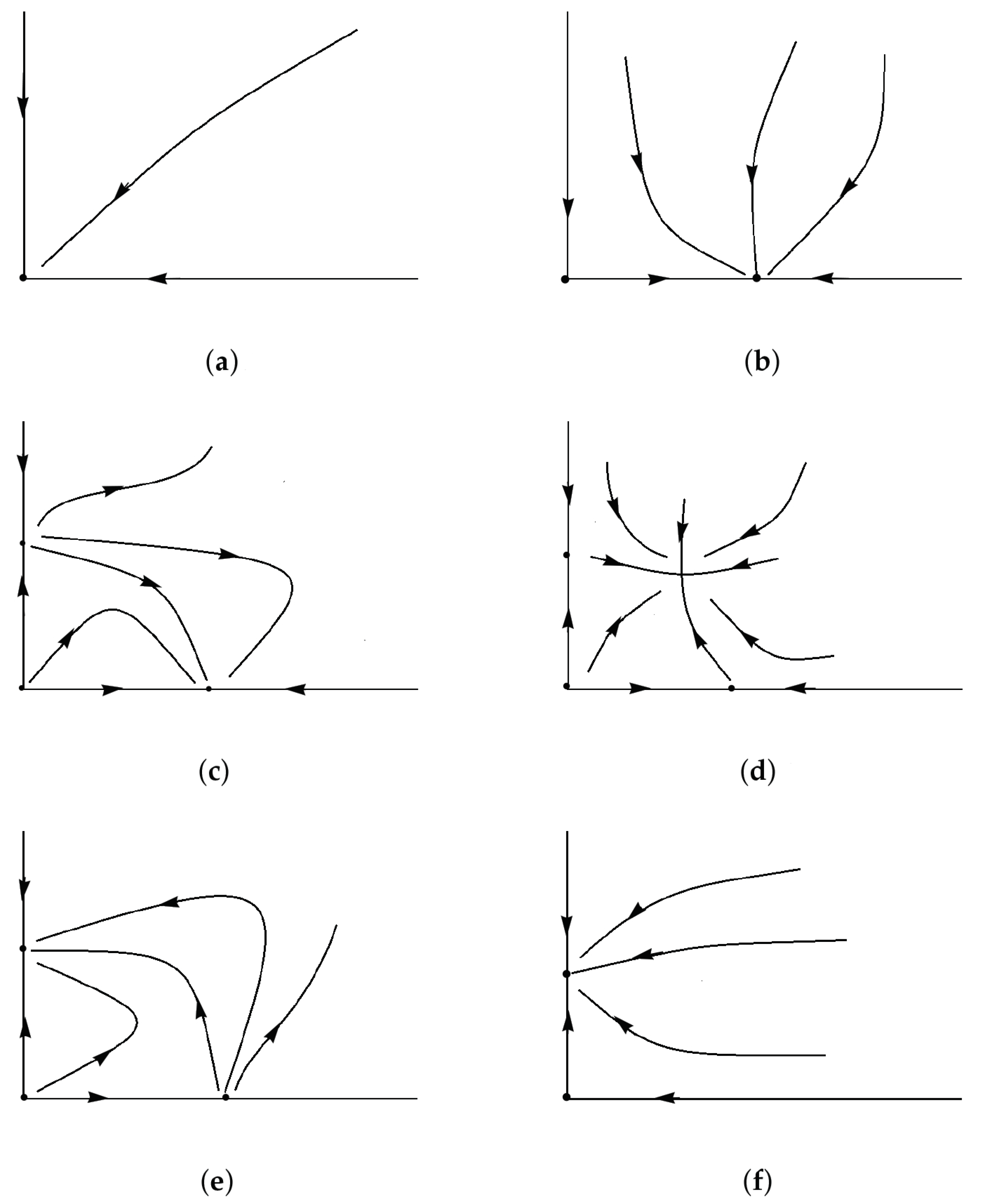
3.2. Classification of Dynamical Behaviours

We take $k=-0.5,\beta =0.4,l=0.5$, and let ${\tau }_1$ and ${\tau }_2$ be the bifurcation parameters. We can draw the curves of Hopf bifurcation when ${\tau }_1,{\tau }_2$ vary. As shown clearly in Figure 4, two Hopf bifurcation curves intersect, and we call the intersections the double Hopf bifurcation point, denoted by HH. It follows that the $({\tau }_2,{\tau }_1)$ plane is divided into different regions, in which the stability of trivial equilibria are different. When the system moves through these curves, the stability switches. Now we take Figure 4b as an example, when ${\tau }_1=1.693,{\tau }_2=0.190$, ${\tau }_{01}^0$, and ${\tau }_{02}^0$ intersect. Figure 5 shows two pairs of pure virtual roots. Correspondingly, $\omega$ can be calculated, and we denote ${\omega }_{11}=0.5731,{\omega }_{12}=0.9424$. Using the central manifold method, we can get

$$\begin{array}{c}\hfill \begin{array}{c}{c}_1=0.1328\epsilon {\delta }_1-0.2735\epsilon {\delta }_2,\hfill \\ c_2=0.0933\epsilon {\delta }_1+0.8495\epsilon {\delta }_2,\hfill \\ a_0=-0.5008,b_0=-0.3969,\hfill \\ c_0=-0.3269,d_0=-0.8860.\hfill \end{array}\end{array}$$

(31)

Figure 4. When $k=-0.5,\beta =0.4,l=0.5$, (a) is the bifurcation set diagram with ${\tau }_2$ as the x-axis and ${\tau }_1$ as the y-axis, and (b) is the partial enlarged diagram and the double Hopf bifurcation point.

Figure 5. When ${\tau }_1=1.693,{\tau }_2=0.190$, two pairs of pure imaginary root eigenvalues at the double Hopf point.

The detailed process can be referred to in Chapter 7 of the Reference [14]. By classifying the bifurcation solutions, we can clearly analyze the dynamic system near the double Hopf bifurcation point. Let ${\dot{r}}_1=0,{\dot{r}}_2=0$ of Equation (29), where we arrived at

$$\begin{array}{c}\hfill \begin{array}{c}{\displaystyle E_0=(0,0),E_1=(\pm \sqrt{\frac{-c_1}{a_0}},0),E_2=(0,\pm \sqrt{\frac{-c_2}{d_0}}),}\hfill \\ {\displaystyle E_{*}=(\pm \sqrt{\frac{c_2{b}_0-c_1{d}_0}{a_0{d}_0-b_0{c}_0}},\pm \sqrt{\frac{c_0{c}_1-a_0{c}_2}{a_0{d}_0-b_0{c}_0}}).}\hfill \end{array}\end{array}$$

(32)

The value of the equilibrium point depends on $c_1,c_2$ in Equation (30). That is when $c_1,c_2$ changes near the critical value $({\tau }_2^c,{\tau }_1^c)$, and the stability of the equilibrium will change as well. We need to pay attention to the straight lines ${\displaystyle c_2=\frac{c_1{d}_0}{b_0}}$ and ${\displaystyle c_2=\frac{c_0{c}_1}{a_0}}$, because there are different dynamic behaviors on both sides of them. At this time, the neighborhood of $({\tau }_2^c,{\tau }_1^c)$ is divided into several parts, including region $I-VI$:

$$\begin{array}{c}\hfill \begin{array}{c}I=\{({\tau }_2^c,{\tau }_1^c)\mid c_1<0,c_2<0\},II=\{({\tau }_2^c,{\tau }_1^c)\mid c_1>0,c_2<0\},\hfill \\ {\displaystyle III=\{({\tau }_2^c,{\tau }_1^c)\mid c_1>0,0<c_2<\frac{c_0{c}_1}{a_0}\},IV=\{({\tau }_2^c,{\tau }_1^c)\mid c_1>0,\frac{c_0{c}_1}{a_0}<c_2<\frac{d_0{c}_1}{b_0}\},}\hfill \\ {\displaystyle V=\{({\tau }_2^c,{\tau }_1^c)\mid c_1>0,c_2>\frac{d_0{c}_1}{b_0}>0\},VI=\{({\tau }_2^c,{\tau }_1^c)\mid c_1<0,c_2>0\}.}\hfill \end{array}\end{array}$$

(33)

We study the normal form of System (29), which is reduced by the central manifold of Equation (11). It can reflect some properties of System (11). Now, Figure 6 shows the area division of the $c_1-c_2$ and ${\tau }_2-{\tau }_1$ planes at the critical point $({\tau }_2^c,{\tau }_1^c)$. In addition, Figure 7 is a phase diagram of different regions.

Figure 6. Classification of the double Hopf bifurcation in (a) $c_1-c_2$; (b) ${\tau }_2-{\tau }_1$.

Figure 7. Bifurcation sets of the solutions derived from the double Hopf bifurcation in the $c_1-c_2$ plane. (a) Region I, (b) Region II, (c) Region III, (d) Region IV, (e) Region V, (f) Region VI in Figure 6, respectively.

Hence, the phase diagrams of different regions are as follows:

When $({\tau }_2,{\tau }_1)$ is in Region I, Equation (29) shows a stable equilibrium point $E_0=(0,0)$, and this area is called the amplitude death region.

When $({\tau }_2,{\tau }_1)$ enters Region II, the equilibrium point $E_0=(0,0)$ becomes a saddle point and produces a new equilibrium point ${\displaystyle E_1=(\sqrt{\frac{-c_1}{a_0}},0)}$, which is stable.

When $({\tau }_2,{\tau }_1)$ is in Region III, the equilibrium point $E_0,E_1$ still exists, and a new equilibrium $E_2$ appears. At this time, $E_0$ is unstable, $E_1$ is stable, and $E_2$ is a saddle.

When $({\tau }_2,{\tau }_1)$ enters Region IV, it is different from Region III. There appears a new equilibrium point, which is expressed as $E_{*}$. $E_0$, $E_1$, and $E_2$ are unstable and $E_{*}$ is stable in this case.

When $({\tau }_2,{\tau }_1)$ is in Region V, $E_{*}$ disappears and there are two other equilibria left. $E_0,E_1$ remain unstable, and $E_2$ becomes stable.

When $({\tau }_2,{\tau }_1)$ enters the last Region VI, the dynamical properties are similar to Region II. The equilibrium $E_0$ is unstable, but $E_2$ is stable.

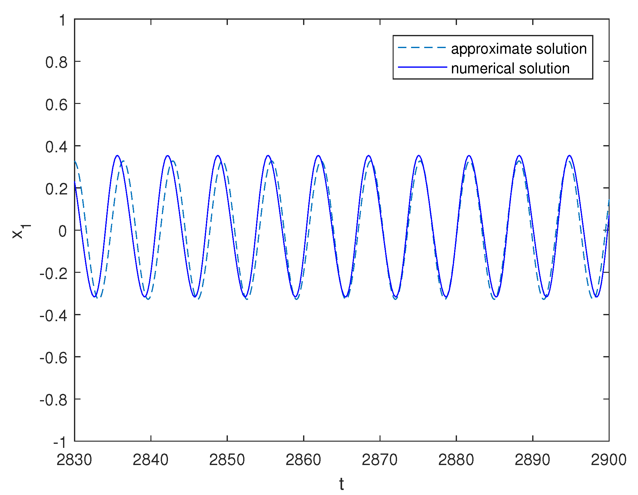
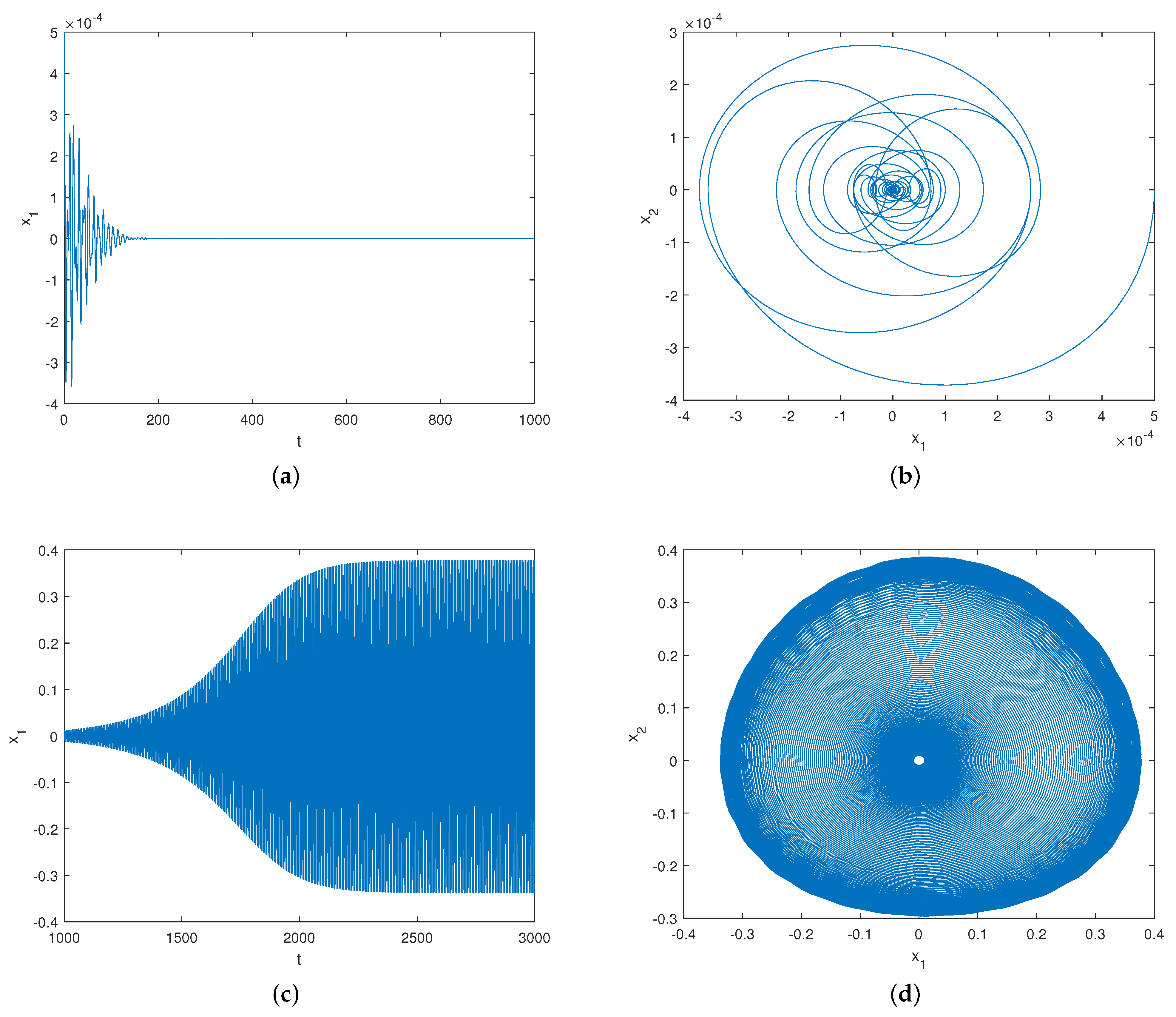
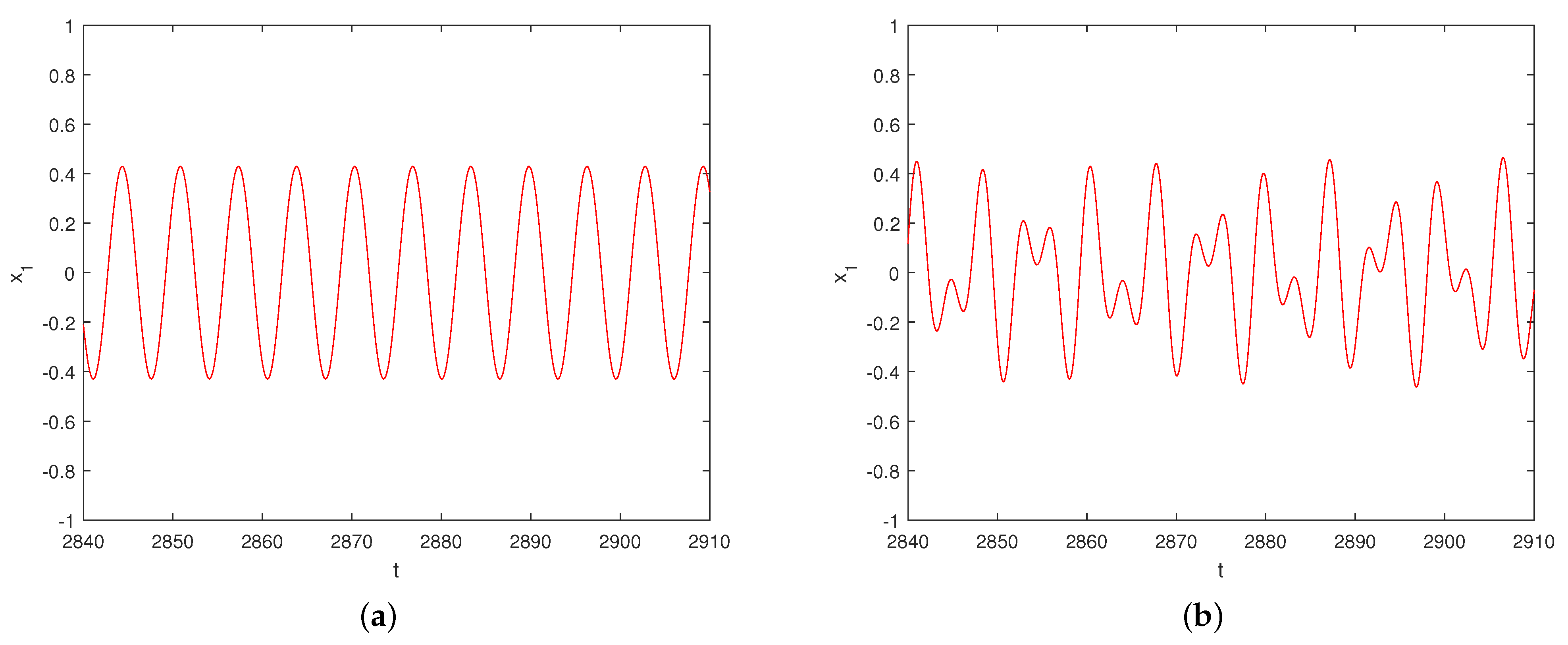
3.3. Numerical Simulation

Due to the instability limit cycle generated by the system, the Runge Kutta method could not be calculated for numerical simulation in the case. Therefore, we could deduce the approximate analytical formula of the limit cycle of the System (2) by $x=\Phi Z$. Figure 8 shows the comparison between the approximate analytical formula (red) and numerical solution (blue). It can be seen that when the parameter is closed to the bifurcations of double Hopf, the approximate solution is in good agreement with the numerical solution. It is worth noting that the accuracy of the approximate solution of the system will decrease rapidly when the parameter selection is far away from the double Hopf bifurcation point. When ${\tau }_1=1.52,{\tau }_2=0.25$, the approximate analytical solution of $x_1$ can be expressed as follows:

$$\begin{array}{c}\hfill \begin{array}{c}{x}_1\left(t\right)=0.3276cos(0.9703t+\theta ),\hfill \end{array}\end{array}$$

(34)

where $\theta$ depends on the initial value.

Figure 8. Comparison of the approximate analytical solution and numerical solution. The dotted line represents the approximate analytical solution, and the solid line represents the numerical solution.

Now we give a numerical simulation. We choose points $(1.4,0.1),(1.52,0.25),(1.75,0.1)$,

$(1.8,0.22)$ from each area in Figure 6b, respectively.

Through the phase diagram and time history diagram in Figure 9, it is found that the system is locally asymptotically stable in Region I. With the change of delay ${\tau }_1$, the equilibrium point loses its stability because of the supercritical Hopf bifurcation, and a stable limit cycle appeared in Region VI. Note that the system periodically oscillates with ${\omega }_{01}=0.5637$. When the system is in Region II, the equilibrium point loses its stability again, and it was caused by a subcritical Hopf bifurcation and produced an unstable limit cycle. The system oscillates at ${\omega }_{01}=0.5871$. However, in Area IV, the system is affected by two frequencies, ${\omega }_{01}=0.5695,{\omega }_{02}=0.9602$ (Figure 10b). Due to the unstable limit cycle, it is impossible to simulate the system numerically, so an approximate solution of the system is given by

$$\begin{array}{c}\hfill \begin{array}{c}{x}_1\left(t\right)=0.2490cos\left(0.9642t\right)+0.2170cos\left(1.6256t\right).\hfill \end{array}\end{array}$$

(35)

Figure 9. The time history diagram and phase diagram of the system. (a,b) Region I in Figure 6, (c,d) Region VI in Figure 6.

Figure 10. The time history diagram of approximate solutions. (a) Region II, (b) Region IV in Figure 6b, respectively.

4. Conclusions

Time delay is an inevitable factor in practice. However, in engineering, more attention is being paid to the phenomenon, and few people study the underlying mechanism theoretically. This paper discussed a type of two-degree-of-freedom van der Pol oscillator with time delay feedback. It was analyzed by using the normal form theory and central manifold theory. Research shows that the time delay transition can cause the stability of the system to switch. Moreover, the greater the time delay, the more complicated the stability switches. Secondly, there are abundant dynamic behaviors near the double Hopf bifurcation. According to the stability of the equilibria, it can be divided into six regions, including the amplitude dead zone and limit cycle zone. It should be noted that, due to the subcritical Hopf bifurcation in the system, it will lead to unstable limit cycles. The Runge Kutta method cannot directly calculate the numerical solution, and the approximate analytical solution of the system can be derived by using the central manifold method.

References

- Ouyang, D.Q.; Shao, J.; Jiang, H.J.; Nguang, S.K.; Shen, H.T. Impulsive synchronization of coupled delayed neural networks with actuator saturation and its application to image encryption. Neural Netw. 2020, 128, 158–171. [Google Scholar] [CrossRef] [PubMed]
- Wang, K.; Yan, X.P.; Yang, Q.; Hao, X.H.; Wang, J.T. Weak Signal Detection Based on Strongly Coupled Duffing-Van der Pol Oscillator and Long Short-term Memory. J. Phys. Soc. Jpn. 2020, 1, 014003. [Google Scholar] [CrossRef]
- Dal, F. The Method of Multiple Time Scales and Finite Differences Method for the van der Pol Oscillator with Small Fractional Damping. Asian Res. J. Math. 2017, 2, 1–11. [Google Scholar] [CrossRef]
- Dong, Y.K.; Wang, D.; Cui, L. Correction to: Assessment of depth-averaged method in analysing runout of submarine landslide. Landslides 2020, 17, 557–565. [Google Scholar] [CrossRef] [Green Version]
- Belhaq, M.; Ghouli, Z.; Hamdi, M. Energy harvesting in a Mathieu–Cvan der Pol–CDuffing MEMS device using time delay. Nonlinear Dyn. 2018, 94, 2537–2546. [Google Scholar] [CrossRef]
- Yang, R.Z.; Zhang, C.R. Dynamics in a diffusive modified Leslie–CGower predator–Cprey model with time delay and prey harvesting. Nonlinear Dyn. 2017, 87, 863–878. [Google Scholar] [CrossRef]
- Shi, J.F.; Gou, X.F.; Zhu, L.Y. Bifurcation of multi-stable behaviors in a two-parameter plane for a non-smooth nonlinear system with time-varying parameters. Nonlinear Dyn. 2020, 100, 3347–3365. [Google Scholar] [CrossRef]
- Stankevich, N.V.; Kuznetsov, A.P.; Seleznev, E.P. Quasi-periodic bifurcations of four-frequency tori in the ring of five coupled van der Pol oscillators with different types of dissipative coupling. Tech. Phys. 2017, 62, 971–974. [Google Scholar] [CrossRef]
- Bukh, A.V.; Anishchenko, V.S. Spiral, Target, and Chimera Wave Structures in a Two-Dimensional Ensemble of Nonlocally Coupled van der Pol Oscillators. Tech. Phys. Lett. 2019, 45, 675–678. [Google Scholar] [CrossRef]
- Singh, A.K.; Yadava, R.D.S. Transient motion and chaotic dynamics in a pair of van der Pol oscillators. Eur. Phys. J. Plus 2019, 134, 1–10. [Google Scholar]
- Algaba, A.; Chung, K.W.; Qin, B.W.; Rodriguez-Luis, A.J. Analytical approximation of the canard explosion in a van der Pol system with the nonlinear time transformation method. Phys. D Nonlinear Phenom. 2020, 406, 132384. [Google Scholar] [CrossRef]
- Qian, Y.H.; Fu, H.X. Research for Coupled van der Pol Systems with Parametric Excitation and Its Application. Z. für Naturforschung 2017, 72, 1009–1020. [Google Scholar] [CrossRef]
- Kumar, M.; Varshney, P. Numerical Simulation of Van der Pol Equation Using Multiple Scales Modified Lindstedt–Poincare Method. Proc. Natl. Acad. Sci. India Sect. A Phys. Sci. 2020, 67, 1–11. [Google Scholar] [CrossRef]
- Guckenheimer, J.; Holmes, P. Nonlinear Oscillations, Dynamical Systems, and Bifurcations of Vector Fields. Appl. Math. Sci. 1983, 42, 353–411. [Google Scholar]
- Peng, M.; Zhang, Z.D.; Qu, Z.F.; Bi, Q.S. Qualitative analysis in a delayed Van der Pol oscillator. Phisica A Stat. Mech. Its Appl. 2020, 554, 123482. [Google Scholar] [CrossRef]
- Sidorov, N.A. Explicit and implicit parametrizations in the construction of branching solutions by iterative methods. Sb. Math. 1995, 186, 297–310. [Google Scholar] [CrossRef]
- Sidorov, N.A.; Leont’ev, R.Y.; Dreglya, A.I. On small solutions of nonlinear equations with vector parameter in sectorial neighborhoods. Math. Notes 2012, 91, 90–104. [Google Scholar] [CrossRef]
- Chen, Z.; Yu, P. Double-Hopf bifurcation in an oscillation with external forcing and time-delayed feedback control. Int. J. Bifurc. Chaos Appl. Sci. Eng. 2006, 16, 3523–3537. [Google Scholar] [CrossRef] [Green Version]
- Du, Y.F.; Niu, B.; Guo, Y.X.; Wei, J.J. Double Hopf Bifurcation in Delayed reaction-diffusion Systems. J. Dyn. Differ. Equ. 2020, 32, 313–358. [Google Scholar] [CrossRef] [Green Version]
- Song, Z.G.; Xu, J. Bifurcation and chaos analysis for a delayed two-neural network with a variation slope ratio in the activation function. Int. J. Bifurc. Chaos Appl. Sci. Eng. 2012, 22, 1250105. [Google Scholar] [CrossRef]
- Ge, J.H.; Xu, J. Fold-Hopf bifurcation in a simplified four-neuron BAM (bidirectional associative memory) neural network with two delays. Sci. China Technol. Sci. 2010, 53, 633–644. [Google Scholar] [CrossRef]
- Qian, Y.H.; Fu, H.X.; Guo, J.M. Weakly resonant double Hopf bifurcation in coupled nonlinear systems with delayed freedback and application of homotopy analysis method. J. Low Freq. Noise Vib. Act. Control 2019, 38, 1651–1675. [Google Scholar] [CrossRef]
- Song, Z.G.; Xu, J. Stability switches and double Hopf bifurcation in a two-neural network system with multiple delays. Cogn. Neurodynamics 2013, 7, 505–521. [Google Scholar] [CrossRef] [PubMed] [Green Version]
- Song, Z.G.; Xu, J. Stability switches and multistability coexistence in a delay-coupled neural oscillators system. J. Theor. Biol. 2012, 313, 98–114. [Google Scholar] [CrossRef]
- Song, Z.G.; Xu, J. Codimension-two bursting analysis in the delayed neural system with external stimulations. Nonlinear Dyn. 2012, 67, 309–328. [Google Scholar] [CrossRef]
- Song, Z.G.; Wang, C.H.; Zhen, B. Codimension-two bifurcation and multistability coexistence in an inertial two-neuron system with multiple delays. Nonlinear Dyn. 2016, 85, 2099–2113. [Google Scholar] [CrossRef]
- Engelborghs, K.; Luzyanina, T.; Roose, D. Numerical bifurcation analysis of delay differential equations using DDE_BIFTOOL. ACM Trans. Math. Softw. 2002, 28, 1–21. [Google Scholar] [CrossRef]
Publisher’s Note: MDPI stays neutral with regard to jurisdictional claims in published maps and institutional affiliations. |
© 2021 by the authors. Licensee MDPI, Basel, Switzerland. This article is an open access article distributed under the terms and conditions of the Creative Commons Attribution (CC BY) license (https://creativecommons.org/licenses/by/4.0/).