Article

Numerical Simulation of Higher-Order Nonlinearity of Human Brain Functional Connectivity Using Hypergraph p-Laplacian

College of Control Science and Engineering, China University of Petroleum, Qingdao 266580, China
*
Author to whom correspondence should be addressed.
Mathematics 2021, 9(18), 2345; https://doi.org/10.3390/math9182345
Submission received: 10 August 2021 / Revised: 15 September 2021 / Accepted: 18 September 2021 / Published: 21 September 2021
(This article belongs to the Section Engineering Mathematics)

Abstract

:
Unravelling how the human brain structure gives rise to function is a central question in neuroscience and remains partially answered. Recent studies show that the graph Laplacian of the human brain’s structural connectivity (SC) plays a dominant role in shaping the pattern of resting-state functional connectivity (FC). The modeling of FC using the graph Laplacian of the brain’s SC is limited, owing to the sparseness of the Laplacian matrix. It is unable to model the negative functional correlations. We extended the graph Laplacian to the hypergraph p-Laplacian in order to describe better the nonlinear and high-order relations between SC and FC. First we estimated those possible links showing negative correlations between the brain areas shared across subjects by statistical analysis. Then we presented a hypergraph p-Laplacian model by embedding the two matrices referring to the sign of the correlations between the brain areas relying on the brain structural connectome. We tested the model on two experimental connectome datasets and evaluated the predicted FC by estimating its Pearson correlation with the empirical FC matrices. The results showed that the proposed diffusion model based on hypergraph p-Laplacian can predict functional correlations more accurately than the models using graph Laplacian as well as hypergraph Laplacian.

1. Introduction

Humans still know little regarding how the human brain works out cognitive tasks, due to its complex structure [1,2], in which hundreds of thousands of neurons, sets of neural populations and multiple brain regions are interconnected and interact together to yield diverse functions in the brain, both in the absence of external stimuli and performing cognitive tasks. Yet, the underlying mechanism behind this still remains incompletely understood. In the last decade, a growing body of research has been performed to explore the relationship between SC and FC with the help of two different kinds of invasive neuroimaging methods, diffusion magnetic resonance imaging (dMRI) measuring the fiber tracts of the white matter between brain regions [3,4] and functional magnetic resonance imaging (fMRI) recording the blood oxygenation level-dependent (BOLD) signals that characterize ongoing neural activities [5,6].
In the last decade, a great number of studies have been conducted to predict the human brain’s SC using resting-state FC, such as network models on the basis of graph measures, neural mass models (NMMs) that describe the neural activity with partial differential equations, and learning-based regression models explicitly mapping FC from SC. The network models usually regard the brain as a graph in which the brain regions are treated as nodes and the connections between regions are defined as edges. A number of network metrics, such as node degrees [7,8], shortest path [9], as well as search information and path transitivity [10], etc., have been used to establish the relation between SC and resting-state FC. These models can only partially capture the nature of FC. Neural mass models [11,12,13] are used to mimic the interactions between neurons in the brain, without considering the signal exchanges between network modules, in which tens of physiological parameters need to be specified prior to obtaining the optimal solution. The regression learning models [14,15,16] simply relate SC with FC using weighted regression, in which the weights are trained using part of the empirical data. Nevertheless, the learned weight coefficients are only effective for the trained dataset while failing to extend to other datasets.
Some studies show that the graph Laplacian of the human brain’s SC has been found to be able to highly capture the relationship between SC and FC, such as the graph diffusion (GD) model [17,18] proposed by Abdelnour, et al. and the hypergraph diffusion (HGD) model [19] proposed by us, in which the FC is described as an exponential decay function [20] of the Laplacian of SC. However, the GD model can yield merely the positive correlations in FC since the graph Laplacian reflects merely the direct connectivity between brain regions. The HGD model, defined by the hypergraph representation of SC, can capture more connection information than SC, thus showing better performance than GD model. However, the modeling of FC using the hypergraph Laplacian of the brain’s SC is also limited to capturing the high-order and nonlinear relation between SC and FC, since the hypergraph Laplacian matrix is still sparse.
To overcome the limitations of GD and HGD models, we extend the graph Laplacian to hypergraph p-Laplacian, which better preserves the local structure [21] and has been successfully applied in pattern recognition and image processing [22,23]. The proposed hypergraph p-Laplacian diffusion model, termed as the HpGD model, is capable of better capturing the high-order relation between SC and FC, demonstrating better performance than GD and HGD models on simulating FC, including the modeling of the negative correlations.
The remainder of the paper is structured as follows. Section 2 gives the notations of the hypergraph network of the human brain adopted in this paper. In Section 3, the HGD model is first introduced in brief then the proposed HpGD model is presented in detail. Section 4 demonstrates comprehensive experiments on two empirical datasets and is following by some discussions in Section 5.

2. Hypergraph Network Notation of the Human Brain

The hypergraph representation of human brain is defined as G = ( V , E , W ) , where V = v i   i   =   1 ,   2 ,   ,   n   is a set of n vertices referring to grey matter brain areas, E represents a set of m hyperedges, E = e j   j   =   1 ,   2 ,   ,   m , in which each hyperedge is composed of several brain areas, v k ( k = 1 , 2 , , n ) , that connect to the corresponding brain area v j , and W = w j   j   =   1 ,   2 ,   ,   m corresponds the weights of each hyperedge defined by summing all the edge weights in the hyperedge.
According to the above notations, we can define the incidence matrix of G by a V × E matrix H , in which H i j = h   ( v i , e j ) = 1 if v i is a vertex of hyperedge e j and 0 otherwise. The degree of a vertex v V in the hypergraph is defined as d v ( v ) =   e E w   ( e )   h   ( v , e ) , while the degree of a hyperedge e E in the hypergraph is defined by δ ( e ) =   v V h   ( v , e ) . Let D v and D e denote the diagonal vertex degree matrix and hyperedge degree matrix, respectively, and W d indicates the diagonal matrix containing the weights of each hyperedge. Then the normalized hypergraph Laplacian can be expressed as L = I D v 1 / 2 H W d D e 1 H T D v 1 / 2 while W h p = H W d H T D v is defined as the adjacency matrix of the hypergraph G . It is worth mentioning that L = I 1 2 D v 1 / 2 H W d H T D v 1 / 2 for the case of simple graph when the hyperedge degree matrix D e reduces to 2 I [24].

3. The Hypergraph p-Laplacian Diffusion Model

3.1. The Hypergraph Laplacian Diffusion Model

In what follows, we briefly describe the hypergraph diffusion model (HGD) in our recent work [19]. Firstly, consider an isolated cortical region v i . There are k ( k = 1 , 2 , , n ) brain areas linking to the brain area v i via edges, with p ( p = 1 , 2 , , k ) brain areas, v k p , with positive correlations and q ( q = 1 , 2 , , k ) brain areas, v k q , with negative correlations to v i , respectively, where k = p + q . Then the first-order dynamics of the signal transmission between cortical regions v i and all the other brain regions ( v j ) can be modified as
d x i ( t ) d t = β d v v i 1 / 2 j = 1 m k = 1 n h ( v i , e j ) w ( e j ) δ e j 1 h ( v k p , e j ) h ( v k q , e j ) d v v k 1 / 2 x k ( t ) x i ( t )
where β is the decay rate. Assume that M p indicates the matrix whose entries are 1 if the correlations between brain areas are positive, otherwise 0, while M q indicates the matrix whose entries are 1 if the correlations between brain areas are negative, otherwise 0, M q = 1 M p . Then the hypergraph network dynamics between all the brain regions can be depicted as
d x ( t ) d t = β D v 1 / 2 H W d D e 1 H T ( M p M q ) D v 1 / 2 I x ( t )
where M p and M q can be estimated by analyzing the averaged experiment FC matrices, respectively. “ ” denotes the Hadamard product.
The solution to the above equation can be solved, i.e.,
x ( t ) = e x p ( β     L ( M p M q ) t ) x 0
where L = I D v 1 / 2 H W d D e 1 H T D v 1 / 2 is the normalized hypergraph network Laplacian.
Suppose the initial condition x 0 = I , then the above solution can be used to simulate the functional interactions between brain areas.

3.2. The Hypergraph p-Laplacian Diffusion Model

Recently, the p-Laplacian has been found to be able to describe the nonlinear relationship in a graph and exhibit better performance than Laplacian in image classification [21]. To this end, we extend the Laplacian in the above model to p-Laplacian and the hypergraph p-Laplacian diffusion (HpGD) model can be formulated as:
x ( t ) = e x p ( β     L p ( M p M q ) t )
where L p denotes the hypergraph p-Laplacian, which satisfies,
g T L p     g = i j w i   j h   p g ( v i ) g ( v j ) p
where g ( ) is a real-valued function defined on the vertices of a weighted hypergraph G, and w i   j h   p W h p denotes the weight strength between vertex i and j in the hypergraph.
The detailed calculation of the hypergraph p-Laplacian is presented in the following section.

3.3. The Computation of Hypergraph p-Laplacian

For any given p, it is complex and difficult to directly obtain the hypergraph p-Laplacian matrix L p from Equation (5). Here we propose an alternative approach to determine L p by eigen-decomposition.
Assume that there are n eigenvectors Γ = f 1 , f 2 , , f n for hypergraph p-Laplacian corresponding to n eigenvalues λ = ( λ 1 , λ 2 , , λ n ) , the hypergraph p-Laplacian matrix expresses by L p = Γ     λ     Γ 1 . Thus, it is crucial to estimate all eigenvectors and eigenvalues for the hypergraph p-Laplacian.
Thomas et al. [21] proposed a method to define the eigenvectors and eigenvalues for the nonlinear operator L p . The real number λ p is named as an eigenvalue of the operator L p if the function f : V satisfies the relationship:
( L p   f ) v i = λ p φ p f v i
where φ p is defined by φ p ( x ) = x p 1 s i g n ( x ) , and the function f is called an eigenvector of L p corresponding to the eigenvalue λ p . When p = 2, the operator L p is equivalent to the standard hypergraph Laplacian L .
According to Equation (5), define K p ( f ) : = f T L p f .
K p ( f ) : = f T L p f = i , j w i j h p f v i f v j p
Similarly, a functional F p : V is defined as
F p ( f ) : = K p ( f ) f p p
where f p p : = v i V f ( v i ) p .
From the Theorem 3.1 in [21] we learned that the functional F p has a critical point at f V if, and only if f is a p-eigenfunction of L p . The corresponding eigenvalue λ p is given as λ p = F p ( f ) . Moreover, we have F p ( α f ) = F p ( f ) for all f V and α .
The above theorem can be applied to the computation of p-Laplacian. It is extremely time-consuming, which limits its applications. Here we propose an efficient approximation algorithm by converting the problem of complex solving eigenvectors into the following optimizing problem:
m i n Γ J ( Γ ) = k F p ( f k ) s . t . v i V φ p ( f v i k ) φ p ( f v i l ) = 0 , k l
where Γ = ( f 1 , f 2 , , f n ) denotes the optimal approximate eigenvector of L p .
According to Equations (7) and (8), it is equivalent to:
m i n Γ J E ( Γ ) = k i , j w i   j h   p f v i k f v j k p f k p p s . t . Γ T Γ = I
where Γ is the eigenvector matrix of the optimal approximate L p . Since the partial derivative with respect to f v i k can be written as,
J E f v i k = 1 f k p p v j V w i   j h   p φ p ( f v i k f v j k ) φ p ( f v i k ) f k p p ,
then the gradient change can be obtained from Equation (10), as follows,
G = J E Γ Γ J E Γ T Γ .
Meanwhile, the eigenvalues λ = ( λ 1 , λ 2 , , λ n ) can be obtained by
λ k = i , j w i   j h   p f v i k f v j k p f k p p .
Finally, the hypergraph p-Laplacian can be approximated by the eigenvalues and eigenvectors.
L p = Γ     λ       Γ 1 .
The estimation algorithm for hypergraph p-Laplacian is summarized in Algorithm 1, in which the step length α is chosen by α   =   β   i   k Γ i   k i   k G i   k , where β is a parameter to control the step length.
Algorithm 1 The estimation of hypergraph p-Laplacian
Input: The structural connectivity network and three parameters k ,   p ,   β
Output: Hypergraph p-Laplacian: L p
Step 1: Initialize the hypergraph Laplacian matrix L and adjacent matrix W h p from the
   structural connectivity network.
Step 2: Decomposition of the hypergraph Laplacian: L = X   λ   X 1 .
Initialize: Γ = X ( : , 1 : k ) .
Step 3: While not converged do:
    G = J E Γ Γ J E Γ T Γ , where J E Γ is given by Equation (10)
    Γ = Γ α G
   End
Step 4:   λ k = i , j w i j h p f v i k f v j k p f k p p
Return:   L p = Γ   λ   Γ 1

4. Experiments

We demonstrate the performance of the extended HpGD model in contrast to the GD model and HGD model in predicting FC. Two commonly used experiment datasets, one with 90 regions of interest (ROIs) derived from eight subjects [17,18] and another with 246 ROIs derived from 50 subjects [25,26], are employed to test the models. The FC and SC of all subjects are rendered as two connectome matrices, with each element in the FC matrix representing the Pearson’s correlation coefficients. Assume that X and Y are BOLD time series of two brain areas recorded using fMRI at rest, each time series has M points, then the Pearson correlation between the two brain areas is calculated by
R = M X i Y i X i Y i M X i 2 ( X i ) 2 M Y i 2 ( Y i ) 2
Note that all the p values of the correlations estimated in our approach are P < < 10 6 .

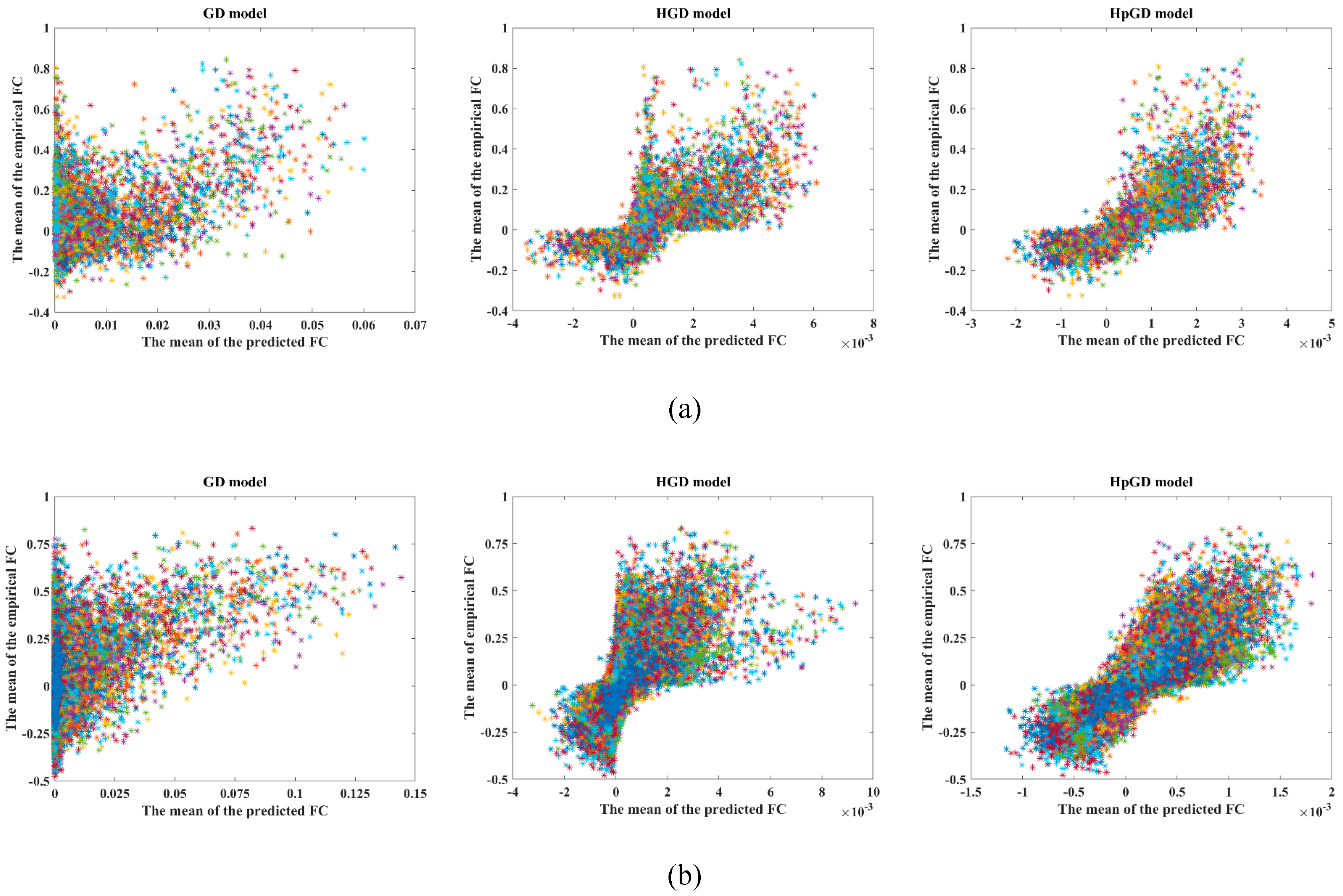
4.1. Correlations with the Experiment FC

For each subject, the prediction result is evaluated using the Pearson correlation between the predicted FC and the empirical FC. The higher of the correlation value is, the more similar the predicted FC is to the empirical FC.
Figure 1 shows the time-varying Pearson correlations between the predicted FC and the empirical FC for each subject of the two datasets using the GD model, HGD model and the proposed HpGD model, respectively. We can observe that the maximum Pearson correlation of the eight subjects of the 90 ROI dataset changed from 0.3735 to 0.4426 for the GD model, 0.4612 to 0.5911 for the HGD model, and 0.4960 to 0.6492 for the HpGD model. The mean correlation values of the three models were 0.4113, 0.5196, and 0.5514, respectively, while the maximum Pearson correlation of the fifty subjects of the 246 ROI dataset changed from 0.3150 to 0.4281 for the GD model, 0.4170 to 0.5436 for the HGD model, and 0.4594 to 0.6547 for the HpGD model. The mean correlation values of the three models are 0.3761, 0.4918 and 0.5789, respectively.
It should be noted that the maximal correlations (critical points) appeared at βtcrit = 2 for the 90 ROIs dataset, βtcrit = 2.5 for the 246 ROIs dataset with the GD model, while at βtcrit = 5 and βtcrit = 5.5 with HGD model and HpGD model, respectively.
Figure 2 demonstrates the scatter plots between the mean predicted FC and the mean empirical FC for the two datasets using the three models. We can observe that the proposed HpGD model showed the best effect in mapping the empirical FC because the relation between the predicted FC using HpGD model and the empirical FC was more linear.

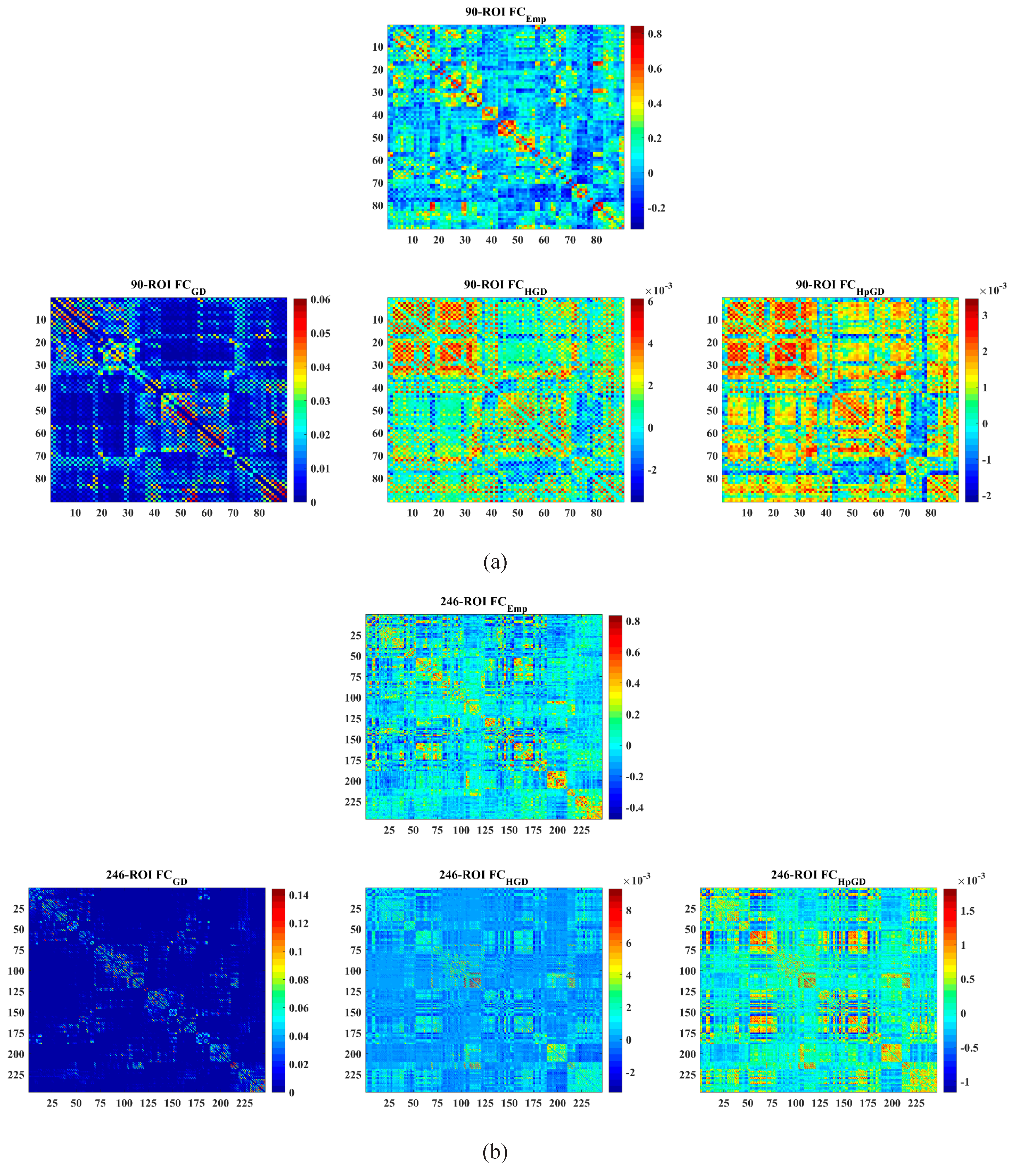
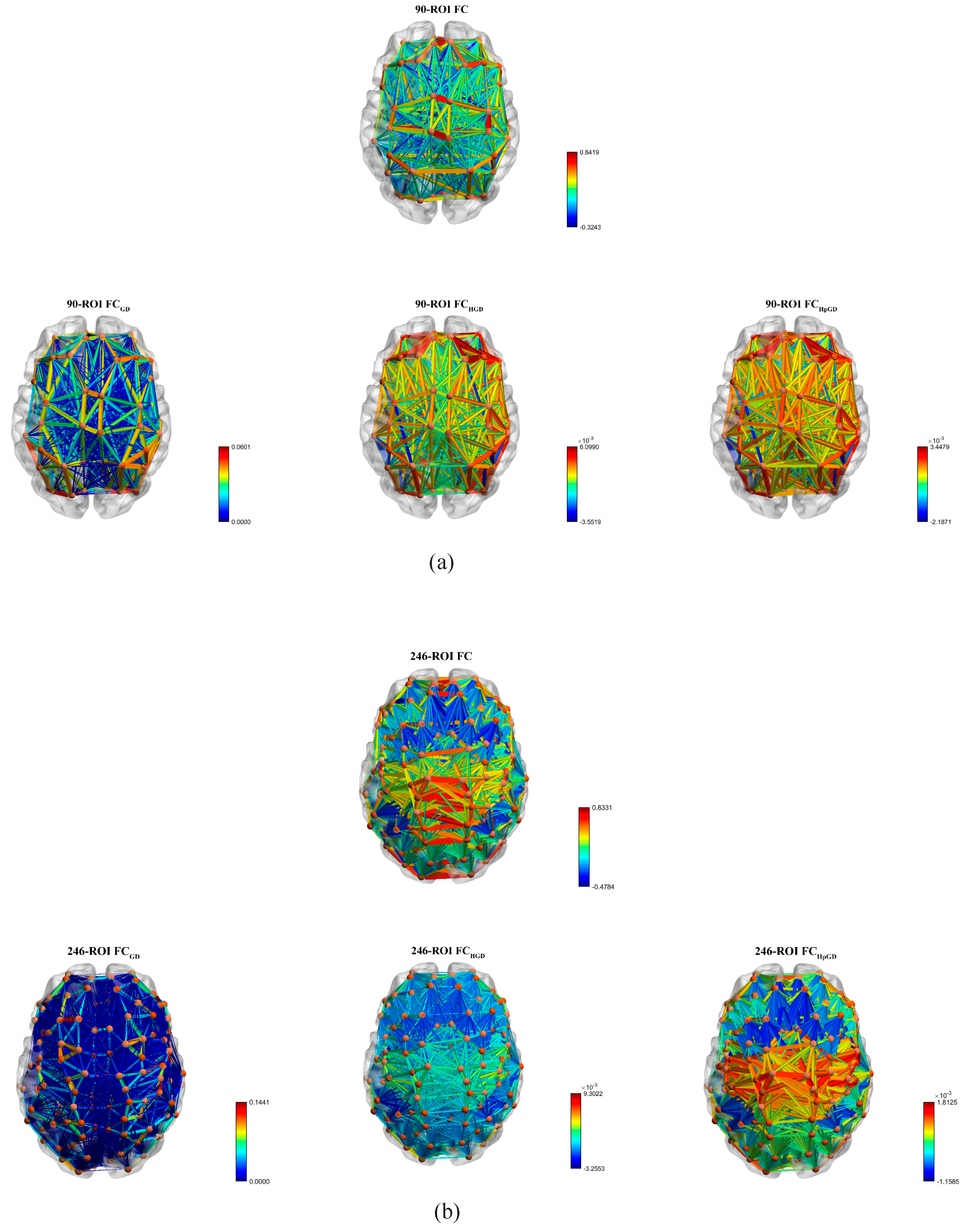
4.2. Mean FC Network

Figure 3 shows the mean predicted FC in contrast to the mean empirical FC rendered as a matrix using the three models, respectively. Figure 4 shows the mean predicted FC in contrast to the mean empirical FC rendered as a network [27] using the three models. It can be clearly observed that the FC predicted by the proposed HpGD model was much closer to the empirical FC than the other two models.

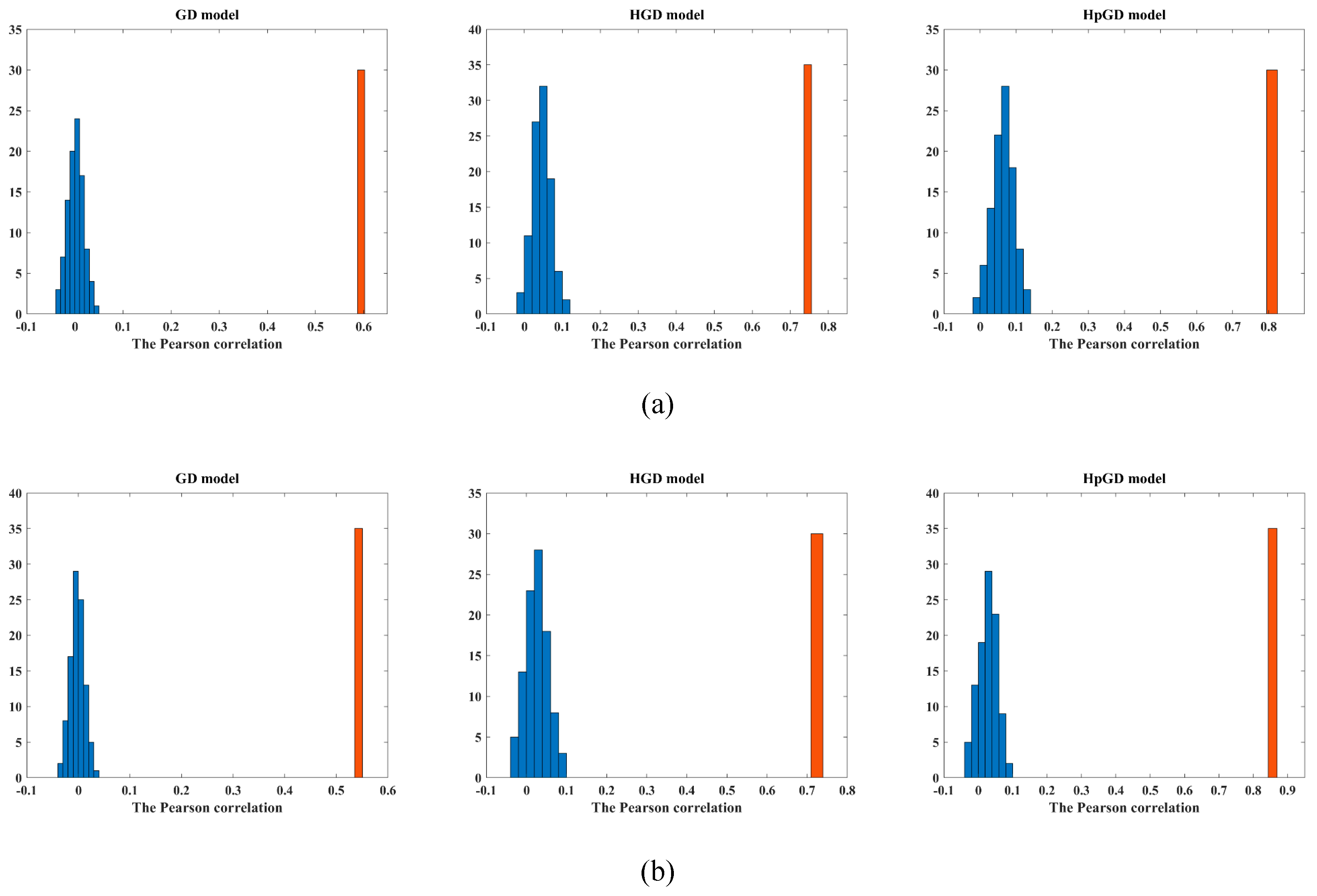
4.3. Stability and Robustness Analysis

To demonstrate that the predicted FC was not acquired by happenstance, for each dataset, we scrambled the mean SC 100 times randomly, then we estimated the FC for each permuted SC matrix with the three models. Figure 5 plots the histogram of the Pearson correlations between the averaged predicted FC and the averaged empirical FC. The histogram of the Pearson correlations without scrambling using the three models is also shown for the two datasets, respectively. The Pearson correlations were calculated between the mean empirical FC and the mean predicted FC (blue) as well as the mean predicted FC without permuting (orange).

5. Conclusions

In this paper, we presented HpGD as an extended graph diffusion model to map FC from SC relying on hypergraph p-Laplacian. HpGD allowed the network to capture the nonlinear and high-order relations between the brain regions. Furthermore, the two matrices that indicate whether the correlations are positive or negative were embedded to entail the model simulating negative functional correlations. To validate the effectiveness of the HpGD model, we performed tests on two experiment connectome datasets with different resolutions. The experimental results from both the 90 ROI dataset and the 246 ROI dataset showed that a hypergraph p-Laplacian-based HpGD model could predict functional correlations more accurately than both the graph Laplacian-based GD model and the hypergraph Laplacian-based HGD model.
However, there are still some limitations. Firstly, the computation of p-Laplacian is time consuming and the three parameters k, p and β need to be optimized beforehand. Secondly, there is still a scarcity of biologically plausible interpretations to the mechanism behind the negative correlations. We will continue to address these issues in our future work.

Author Contributions

Software, J.M.; validation, C.D.; methodology, W.L.; writing—review and editing, Y.W. All authors have read and agreed to the published version of the manuscript.

Funding

This paper was funded by the China Scholarship Council grant No.201306455001, the National Natural Science Foundation of P.R. China grant No.62072468, and the Graduate Innovation Project of China University of Petroleum (East China) grant No. YCX2020095.

Institutional Review Board Statement

Not applicable.

Informed Consent Statement

Not applicable.

Data Availability Statement

Not applicable.

Conflicts of Interest

The authors declare no conflict of interest.

References

  1. Rubinov, M.; Sporns, O. Complex network measures of brain connectivity: Uses and interpretations. NeuroImage 2010, 52, 1059–1069. [Google Scholar] [CrossRef]
  2. Uddin, L.Q. Complex relationships between structural and functional brain connectivity. Trends Cogn. Sci. 2013, 17, 600–602. [Google Scholar] [CrossRef] [Green Version]
  3. Iturria-Medina, Y.; Sotero, R.C.; Canales-Rodrguez, E.J.; Aleman-Gomez, Y.; Melie-Garcia, L. Studying the human brain anatomical network via diffusion-weighted MRI and graph theory. NeuroImage 2008, 40, 1064–1076. [Google Scholar] [CrossRef]
  4. Zhu, D.J.; Zhang, T.; Jiang, X.; Hu, X.T.; Chen, H.B.; Yang, N.; Lv, J.L.; Han, J.W.; Guo, L.; Liu, T.M. Fusing DTI and fMRI data: A survey of methods and applications. NeuroImage 2014, 102, 184–191. [Google Scholar] [CrossRef] [PubMed] [Green Version]
  5. Eavani, H.; Satterthwaite, T.D.; Filipovych, R.; Gur, R.E.; Gur, R.C.; Davatzikos, C. Identifying sparse connectivity patterns in the brain using resting-state fMRI. NeuroImage 2015, 105, 286–299. [Google Scholar] [CrossRef] [PubMed] [Green Version]
  6. Uddin, L.Q.; Mooshagian, E.; Zaidel, E.; Scheres, A.; Margulies, D.S.; Kelly, A.C.; Shehzad, Z.; Adelstein, J.S.; Castellanos, F.X.; Biswal, B.B.; et al. Residual functional connectivity in the split-brain revealed with resting-state functional MRI. Neuroreport 2008, 19, 703–709. [Google Scholar] [CrossRef] [PubMed] [Green Version]
  7. Tewarie, P.; Hillebrand, A.; van Dellen, E.; Schoonheim, M.M.; Barkhof, F.; Polman, C.H.; Beaulieu, C.; Gong, G.; van Dijk, B.W.; Stam, C.J. Structural degree predicts functional network connectivity: A multimodal resting-state fMRI and MEG study. NeuroImage 2014, 97, 296–307. [Google Scholar] [CrossRef]
  8. Stam, C.J.; van Straaten, E.C.W.; van Dellen, E.; Tewarie, P.; Gong, G.; Hillebrand, A.; Meier, J.; Van Mieghem, P. The relation between structural and functional connectivity patterns in complex brain networks. Int. J. Psychophysiol. 2016, 103, 149–160. [Google Scholar] [CrossRef]
  9. Ventrella, A.V.; Piro, G.; Grieco, L.A. On modeling shortest path length distribution in scale-free network topologies. IEEE Syst. J. 2018, 12, 3869–3872. [Google Scholar] [CrossRef]
  10. Goni, J.; van den Heuvel, M.P.; Avena-Koenigsberger, A.; de Mendizabal, N.V.; Betzel, R.F.; Griffa, A.; Hagmann, P.; Corominas-Murtra, B.; Thiran, J.P.; Sporns, O. Resting-brain functional connectivity predicted by analytic measures of network communication. Proc. Natl. Acad. Sci. USA 2014, 111, 833–838. [Google Scholar] [CrossRef] [Green Version]
  11. Honey, C.J.; Sporns, O.; Cammoun, L.; Gigandet, X.; Thiran, J.P.; Meuli, R.; Hagmann, P. Predicting human resting-state functional connectivity from structural connectivity. Proc. Natl. Acad. Sci. USA 2009, 106, 2035–2040. [Google Scholar] [CrossRef] [PubMed] [Green Version]
  12. Deco, G.; Ponce-Alvarez, A.; Mantini, D.; Romani, G.L.; Hagmann, P.; Corbetta, M. Resting-state functional connectivity emerges from structurally and dynamically shaped slow linear fluctuations. J. Neurosci. 2013, 33, 11239–11252. [Google Scholar] [CrossRef] [PubMed]
  13. Messe, A.; Rudrauf, D.; Giron, A.; Marrelec, G. Predicting functional connectivity from structural connectivity via computational models using MRI: An extensive comparison study. NeuroImage 2015, 111, 65–75. [Google Scholar] [CrossRef] [PubMed]
  14. Rosenthal, G.; Vasa, F.; Griffa, A.; Hagmann, P.; Amico, E.; Goni, J.; Avidan, G.; Sporns, O. Mapping higher-order relations between brain structure and function with embedded vector representations of connectomes. Nat. Commun. 2018, 9, 2178. [Google Scholar] [CrossRef]
  15. Surampudi, S.G.; Misra, J.; Deco, G.; Bapi, R.S.; Sharma, A.; Roy, D. Resting state dynamics meets anatomical structure: Temporal multiple kernel learning (tmkl) model. NeuroImage 2019, 184, 609–620. [Google Scholar] [CrossRef] [PubMed]
  16. Chu, S.; Parhi, K.K.; Lenglet, C. Function-specific and enhanced brain structural connectivity mapping via joint modeling of diffusion and functional MRI. Sci. Rep. 2018, 8, 4741. [Google Scholar] [CrossRef] [Green Version]
  17. Abdelnour, F.; Voss, H.U.; Raj, A. Network diffusion accurately models the relationship between structural and functional brain connectivity networks. Neuroimage 2014, 90, 335–347. [Google Scholar] [CrossRef] [Green Version]
  18. Abdelnour, F.; Dayan, M.; Devinsky, O.; Thesen, T.; Raj, A. Functional brain connectivity is predictable from anatomic network’s Laplacian eigen-structure. Neuroimage 2018, 172, 728–739. [Google Scholar] [CrossRef]
  19. Ma, J.C.; Wang, Y.J.; Liu, B.D.; Liu, W.F. Accurately modeling the human brain functional correlations with hypergraph Laplacian. Neurocomputing 2021, 428, 239–247. [Google Scholar] [CrossRef]
  20. Raj, A.; Kuceyeski, A.; Weiner, M. A network diffusion model of disease progression in dementia. Neuron 2012, 73, 1204–1215. [Google Scholar] [CrossRef] [Green Version]
  21. Buhler, T.; Hein, M. Spectral clustering based on the graph p-Laplacian. In Proceedings of the 26th Annual International Conference on Machine Learning, Montreal, QC, Canada, 14–18 June 2009; pp. 81–88. [Google Scholar]
  22. Ma, X.Q.; Liu, W.F.; Li, S.Y.; Tao, D.P.; Zhou, Y.C. Hypergraph p-Laplacian regularization for remotely sensed image recognition. IEEE T. Geosci. Remote. 2019, 57, 1585–1595. [Google Scholar] [CrossRef] [Green Version]
  23. Fu, S.C.; Liu, W.F.; Zhou, Y.C.; Nie, L.Q. HplapGCN: Hypergraph p-Laplacian graph convolutional networks. Neurocomputing 2019, 362, 166–174. [Google Scholar] [CrossRef]
  24. Zhou, D.Y.; Huang, J.Y.; Schölkopf, B. Learning with hypergraphs: Clustering, classification, and embedding. In Proceedings of the 19th International Conference on Neural Information Processing Systems, Vancouver, BC, Canada, 4–7 December 2006; pp. 1601–1608. [Google Scholar]
  25. Lin, Q.X.; Dai, Z.J.; Xia, M.R.; Han, Z.Z.; Huang, R.W.; Gong, G.L.; Liu, C.; Bi, Y.C.; He, Y. A connectivity-based test-retest dataset of multi-modal magnetic resonance imaging in young healthy adults. Sci. Data 2015, 2, 150056. [Google Scholar] [CrossRef] [PubMed] [Green Version]
  26. Fan, L.Z.; Li, H.; Zhuo, J.J.; Zhang, Y.; Wang, J.J.; Chen, L.F.; Yang, Z.Y.; Chu, C.Y.; Xie, S.M.; Laird, A.R.; et al. The human brainnetome atlas: A new brain atlas based on connectional architecture. Cereb. Cortex 2016, 26, 3508–3526. [Google Scholar] [CrossRef]
  27. Xia, M.R.; Wang, J.H.; He, Y. Brainnet viewer: A network visualization tool for human brain connectomics. PLoS ONE 2013, 8, e68910. [Google Scholar] [CrossRef] [Green Version]
Figure 1. The comparison of the Pearson correlations varying with the parameter βt. (a) 90 ROIs dataset ( k = 89 ,   p = 1 ,   β = 0.2 ). (b) The 246 ROIs dataset ( k = 245 ,   p = 1.1 ,   β = 0.2 ).
Mathematics 09 02345 g001
Figure 2. The scatter plots for the two datasets with the three models. (a) The 90 ROIs dataset. (b) The 246 ROIs dataset.
Mathematics 09 02345 g002
Figure 3. The mean empirical FC matrices vs. the mean predicted FC matrices by the three models. (a) The 90 ROIs dataset. (b) The 246 ROIs dataset.
Mathematics 09 02345 g003
Figure 4. The mean empirical FC network vs. the mean predicted FC networks by the three models. (a) The 90 ROIs dataset. (b) The 246 ROIs datasets.
Mathematics 09 02345 g004
Figure 5. The histogram of the Pearson correlations with the three models. (a) The 90 ROIs dataset. (b) The 246 ROIs dataset.
Mathematics 09 02345 g005
Publisher’s Note: MDPI stays neutral with regard to jurisdictional claims in published maps and institutional affiliations.

