Article

Inverse Problem for an Equation of the Reaction-Diffusion-Advection Type with Data on the Position of a Reaction Front: Features of the Solution in the Case of a Nonlinear Integral Equation in a Reduced Statement

1
Department of Mathematics, Faculty of Physics, Lomonosov Moscow State University, 119991 Moscow, Russia
2
Moscow Center for Fundamental and Applied Mathematics, 119234 Moscow, Russia
*
Author to whom correspondence should be addressed.
Mathematics 2021, 9(18), 2342; https://doi.org/10.3390/math9182342
Submission received: 20 August 2021 / Revised: 14 September 2021 / Accepted: 18 September 2021 / Published: 21 September 2021
(This article belongs to the Section Computational and Applied Mathematics)

Abstract

:
The paper considers the features of numerical reconstruction of the advection coefficient when solving the coefficient inverse problem for a nonlinear singularly perturbed equation of the reaction-diffusion-advection type. Information on the position of a reaction front is used as data of the inverse problem. An important question arises: is it possible to obtain a mathematical connection between the unknown coefficient and the data of the inverse problem? The methods of asymptotic analysis of the direct problem help to solve this question. But the reduced statement of the inverse problem obtained by the methods of asymptotic analysis contains a nonlinear integral equation for the unknown coefficient. The features of its solution are discussed. Numerical experiments demonstrate the possibility of solving problems of such class using the proposed methods.

1. Introduction

Problems for nonlinear singularly perturbed reaction-diffusion-advection equations arise in gas dynamics [1], combustion theory [2], chemical kinetics [3,4,5,6,7,8,9,10], nonlinear wave theory [11], biophysics [12,13,14,15,16], medicine [17,18,19,20], ecology [21,22,23,24,25], finance [26] and other fields of science [27]. A specific feature of problems of this type is the presence of processes of different scales. Therefore, the mathematical models of these problems are described by nonlinear parabolic equations with a small parameter at the highest derivative. In this regard, solutions to these problems may contain narrow moving fronts that divide the space into two parts: the disturbed part, through which the front has already passed, and the undisturbed part. The front is a region in which the function describing some characteristic of the medium (temperature, density, etc.) changes quite sharply from the values of the function describing one state of the medium (for example, undisturbed) to the value of the function describing another state. The width of such a front is rather small in relation to the size of the entire region [11]. As a consequence, the reaction front can be distinguished experimentally.
Some applied problems for equations of this type require solving inverse problems for recovering some coefficient in the equation. To formulate the inverse problem, additional information is required, which is usually measured in an experiment. Often, in the formulation of inverse problems for partial differential equations, additional information about the solution on a part of the boundary of the domain is used (see, for example, [24,28,29,30,31,32,33,34,35,36,37]). However, one of the possible statements of inverse problems for equations of the type under consideration is a statement with additional information about the dynamics of the reaction front motion (see, for example, [38,39,40]). Additional data of this type are in demand in practice, since they are most easily to observe in an experiments (the front is an easily distinguishable contrast structure).
The simplest formulation of an inverse problem of this type relates to the case of recovering a function of an argument from experimental observations of a function of the same argument. For example, in [41], an approach was considered to restore the function of a temporary variable argument from the observation data of the function also of the variable argument in time. More complex formulations are formulations in which it is required to restore the function of one argument (for example, spatial) from the observation data of the function of another argument (for example, temporal). This class of inverse problems is considered by the authors recently—the recovering of the function of the argument of a spatial variable (that determines the properties of the medium) from the data of observations of the function of the argument of the time variable (that determined by the dynamics of the reaction front). In this paper, we consider the question of the possibility of recovering the advection coefficient in the generalized Burgers equation [42] from the data on the dynamics of the reaction front.
To effectively solve such inverse problems the methods of asymptotic analysis can be used [3,43]. In such cases, it is possible to reduce the original inverse problem for a nonlinear singularly perturbed partial differential equation to a much simpler problem with respect to the coefficient to be restored. The resulting simplified problem is called as a reduced statement (formulation) of the inverse problem.
However, the reduced formulations of such inverse problems may have special features. It was shown that the reduced formulations can contain (1) algebraic equations for an unknown coefficient (see, for example, [44]), (2) differential equations for an unknown coefficient (see, for example, [40]), (3) integral equations for an unknown coefficient. The first case is the simplest and allows to restore the unknown function only at those points through which the reaction front passed during its experimental observation. In this case, a pointwise recovering of the unknown coefficient is possible. The second case is more complicated, since additional input information is required for the correct formulation of the inverse problem being solved. The third case is the most difficult. In this paper, we consider a more complex example compared to the example discussed in [39]. Now, as a result of applying the asymptotic analysis methods, a nonlinear integral equation arises.
The structure of this work is as follows. Section 2 presents the physical formulation of the inverse problem of determining the advection coefficient in the generalized Burger’s equation with data on the position of the reaction front. As a consequence, an important question arises: is it possible to obtain a mathematical connection between the unknown coefficient and the data of the inverse problem? The methods of asymptotic analysis of the direct problem help to solve this question. Thus, in Section 3 the methods of asymptotic analysis are used in order to obtain the so-called reduced statement of the inverse problem. The next question is: how to solve the obtained equation? Thus, Section 4 describes the features of the numerical search for the unknown solution from the reduced formulation of the inverse problem. The final question is whether the proposed approach can be trusted? Section 5 demonstrates the results of numerical experiments, from which it is possible to draw conclusions about the possibilities and limitations of the proposed approach.

2. Statement of the Inverse Problem

Consider the problem for a nonlinear singularly perturbed Burger’s type equation:
{ ε 2 u x 2 u t = q ( x ) u u x u 3 , x ( 0 , 1 ) , t ( 0 , T ] , u ( 0 , t ) = u l e f t ,     u ( 1 , t ) = u r i g h t , t ( 0 , T ] , u ( x , 0 ) = u i n i t ( x ) , x [ 0 , 1 ] ,
where 0 < ε 1 —is a small parameter, and the functions q ( x ) and u i n i t ( x ) are sufficiently smooth, with q ( x ) > 0 everywhere on the segment x [ 0 , 1 ] .
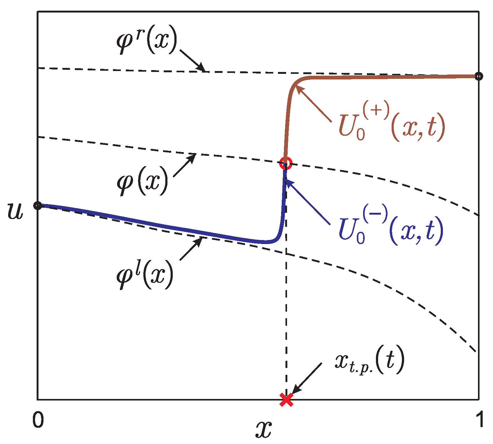
Under certain conditions, the problem (1) can have a solution of the moving front type. A solution of this type is a function that has a narrow interior layer in a small (of the order of ε | ln ε | ) neighborhood of some point, that moving according to the law x = x t . p . ( t ) . We call the point x t . p . ( t ) as “transition poin” (“t.p.”). Outside this neighborhood, the solution is close to one of two functions, φ l ( x ) or φ r ( x ) , each of which is independent of time (see Figure 1).
Remark 1.
There is no need to specify and verify the conditions under which a front-type solution exists. Our aim is to solve the inverse problem. Thus, if we observe a reaction front in an experiment, the conditions for the existence of a front-type solution are satisfied (whatever they may be).
The inverse problem is to determine the coefficient q ( x ) > 0 in (1) from the known additional information about the position of the reaction front
x t . p . ( t ) = f ( t ) ,     t [ 0 , T ] .
Remark 2.
Note that in practice, instead of the exact data f ( t ) , the experimentally measured approximate value f δ ( t ) (see Figure 1) is known, such that:
f f δ L 2 δ .
To solve the inverse problem, an explicit connection between the unknown function q ( x ) and the data of the inverse problem f ( t ) is required. The question arises: whether such a connection can be obtained? The methods of asymptotic analysis, the application of which to the problem (1) is discussed in the next section, will help us solve this question (the result is the Equation (13)).

3. Construction of the Reduced Statement of the Inverse Problem Using the Asymptotic Analysis Methods

We assume that for any x [ 0 , 1 ] , the inequality φ l ( x ) < φ r ( x ) is satisfied. Then the solution is of the front type (if it exists) and it will be increasing over the entire segment x [ 0 , 1 ] at any time t [ 0 , T ] . In order for such a solution of the direct problem (1) to exist, we require the following conditions to be met.
(A1)
Let the initial function u i n i t ( x ) of the problem (1) have the form of a formed front with a large gradient in the vicinity of the point x t . p . ( 0 ) . Let the initial and boundary conditions be consistent to continuity: u i n i t ( 0 ) = u l e f t , u i n i t ( 1 ) = u r i g h t .
(A2)
Let the inequalities φ l ( x ) < 0 , φ r ( x ) > 0 be satisfied everywhere on the segment x [ 0 , 1 ] .
The algorithm from the work [45] based on the methods of asymptotic analysis allows us to obtain an approximate law of motion of the point of localization of the reaction front x = x t . p . ( t ) . In this paper, it is proved that the following representations are valid
u ( x , t ) = U 0 ( x , t ) + O ( ε ) ,     x t . p . ( t ) = x 0 ( t ) + O ( ε ) ,
where U 0 ( x , t ) is the zero-order asymptotic approximation in the small parameter of the solution to the problem (1), and x 0 ( t ) is the zero approximation for the coordinate of the reaction front localization point at time t.
The function U 0 ( x , t ) is constructed separately on each of the sets D ¯ ( ) : = { ( x , t ) [ 0 , x t . p . ( t ) ] × ( 0 , T ] } and D ¯ ( + ) : = { ( x , t ) [ x t . p . ( t ) , 1 ] × ( 0 , T ] } :
U 0 ( x , t ) = { U 0 ( ) ( x , t ) , ( x , t ) D ¯ ( ) , U 0 ( + ) ( x , t ) , ( x , t ) D ¯ ( + ) .
Each of the functions U 0 ( ) ( x , t ) is the sum of two terms: (1) the regular part, the function φ l , r ( x ) , and (2) the transition layer function, Q ( ) ( ξ , x t . p . ( t ) ) , describing the behavior of the solution in the vicinity of the point x t . p . ( t ) at each time instant and depending on the stretched variable ξ = ( x x t . p . ( t ) ) / ε :
U 0 ( ) ( x , t ) = φ l ( x ) + Q ( ) ( ξ , x t . p . ( t ) ) ,     U 0 ( + ) ( x , t ) = φ r ( x ) + Q ( + ) ( ξ , x t . p . ( t ) ) .
These functions satisfy the joining condition at the point x t . p . ( t ) at each moment of time t [ 0 , T ] in such a way that the following condition is fulfilled (see Figure 2)
U 0 ( ) ( x t . p . ( t ) , t ) = U 0 ( + ) ( x t . p . ( t ) , t ) = φ ( x t . p . ( t ) ) ,
where φ ( x ) is defined as
φ ( x ) 1 2 ( φ l ( x ) + φ r ( x ) ) ,     x [ 0 , 1 ] .
Far from the region of localization of the reaction front, the solution of the problem (1) in the zero approximation can be described by the functions of the regular part φ l , r ( x ) . The equations for these functions are obtained from the Equation (1), if we discard the term containing ε and take into account that these functions do not depend on time. According to the algorithm from the work [45] these functions are defined as solutions to the following Cauchy problems:
{ q ( x ) φ l φ l x + ( φ l ) 3 = 0 ,     x ( 0 , 1 ] , φ l ( 0 ) = u l e f t ,
and
{ q ( x ) φ r φ r x + ( φ r ) 3 = 0 ,     x [ 0 , 1 ) , φ r ( 1 ) = u r i g h t .
The solutions to the problems (5) and (6) can be written out explicitly:
φ l ( x ) = 1 1 u l e f t + 0 x d s q ( s ) ,     φ r ( x ) = 1 1 u r i g h t x 1 d s q ( s ) .
Let us define the functions Q ( ) ( ξ , x t . p . ( t ) ) so that the functions U 0 ( ) satisfy the Equation (1) with respect to the residual up to O ( ε 0 ) in the domains D ( ) . To do this, we substitute each of these functions into the Equation (1). At the same time, we note that the differential operators included in this equation are rewritten as follows through the variable ξ :
x = 1 ε · ξ ,     2 x 2 = 1 ε 2 · 2 ξ 2 ,     t = 1 ε · d x t . p . d t · ξ + O ( ε 0 ) .
Combining the terms of the order O ( ε 1 ) , we obtain the following equations for the functions Q ( ) ( ξ , x t . p . ( t ) ) :
2 Q ( ) ξ 2 + x t . p . d t Q ( ) ξ = q ( x t . p . ( t ) + ε ξ ) ( Q ( ) + φ l , r ( x t . p . ( t ) + ε ξ ) ) Q ( ) ξ .
Let us introduce the function
u ˜ ( ξ , x t . p . ( t ) ) : = { Q ( ) ( ξ , x t . p . ( t ) ) + φ l ( x t . p . ( t ) ) , ξ 0 , t ( 0 , T ] , Q ( + ) ( ξ , x t . p . ( t ) ) + φ r ( x t . p . ( t ) ) , ξ 0 , t ( 0 , T ] .
We will define the function u ˜ separately for ξ 0 and ξ 0 from the following problems, in which the variable t ( 0 , T ] is a parameter:
{ 2 u ˜ ξ 2 + x t . p . d t · u ˜ ξ = q ( x t . p . ( t ) ) u ˜ u ˜ ξ ,     ξ 0 , u ˜ ( 0 , x t . p . ( t ) ) = φ ( x t . p . ( t ) ) ,     u ˜ ( , x t . p . ( t ) ) = φ l ( x t . p . ( t ) ) ,
{ 2 u ˜ ξ 2 + x t . p . d t · u ˜ ξ = q ( x t . p . ( t ) ) u ˜ u ˜ ξ ,     ξ 0 , u ˜ ( 0 , x t . p . ( t ) ) = φ ( x t . p . ( t ) ) ,     u ˜ ( + , x t . p . ( t ) ) = φ r ( x t . p . ( t ) ) .
Consider the solutions to the last problems on the phase plane. To do this, we pass from the second-order equation in these problems to the equivalent system of equations
{ u ˜ ξ = Φ ,     ξ ( , + ) , Φ ξ = d x t . p . d t · Φ q ( x t . p . ( t ) ) u ˜ · Φ ,     ξ ( , + ) .
Dividing the second equation of this system by the first, we obtain an equation describing the phase trajectories in the ( u ˜ , Φ ) plane. The points ( φ l , 0 ) and ( φ r , 0 ) of the phase plane are the rest points of the system (11). Let us define the functions Φ ( ) ( ξ , x t . p . ( t ) ) for each value of the parameter t ( 0 , T ] as solutions to Cauchy problems
{ Φ ( ) u ˜ = q ( x t . p . ( t ) ) · u ˜ d x t . p . d t ,     u ˜ ( φ l ( x t . p . ( t ) ) , φ r ( x t . p . ( t ) ) ] , Φ ( ) ( φ l ( x t . p . ( t ) ) ) = 0 ,
and
{ Φ ( + ) u ˜ = q ( x t . p . ( t ) ) · u ˜ d x t . p . d t ,     u ˜ [ φ l ( x t . p . ( t ) ) , φ r ( x t . p . ( t ) ) ) , Φ ( + ) ( φ r ( x t . p . ( t ) ) ) = 0 .
By condition (A2) and q ( x t . p ( t ) ) > 0 , the function Φ ( ) describes a phase trajectory that enters the rest point ( φ l , 0 ) at ξ , and the function Φ ( + ) describes a phase trajectory that enters the rest point ( φ r , 0 ) at ξ + . The initial conditions of these Cauchy problems ensure that the conditions for ξ of the problems (9) and (10) are met, and their solutions can be written out explicitly:
Φ ( ) ( ξ , x t . p . ( t ) ) = q ( x t . p . ( t ) ) 2 ( u ˜ 2 ( φ l , r ( x t . p . ( t ) ) ) 2 ) d x t . p . d t ( u ˜ φ l , r ( x t . p . ( t ) ) ) .
The function x 0 ( t ) is determined from the condition of joining the left and right derivatives of the asymptotic approximation with respect to the variable x at the point x t . p . ( t ) at each moment of time. This condition, taking into account the representation (4), is written as
Q ( ) ξ ( 0 , x t . p ( t ) ) Q ( + ) ξ ( 0 , x t . p ( t ) ) = O ( ε ) .
Substituting here the representation (3) for the function x t . p . ( t ) , taking into account the equality (8), the first equation of the system (11) and leaving only terms of order zero in the Taylor expansion in the parameter ε , we obtain the equality
Φ ( ) ( 0 , x 0 ( t ) ) Φ ( + ) ( 0 , x 0 ( t ) ) = 0 ,
which can be considered an equation for determining the function x 0 ( t ) .
Let us substitute explicit expressions for the functions Φ ( ) into this equation and take into account that at the initial moment of time the front is formed in the vicinity of the point x t . p . ( 0 ) . As a result, we obtain the Cauchy problem, which determines the leading term x 0 ( t ) of the asymptotic approximation in the small parameter ε of the exact position x t . p . ( t ) of the moving front:
{ d x 0 d t = q ( x 0 ) 2 ( φ r ( x 0 ) + φ l ( x 0 ) ) ,     t ( 0 , T ] , x 0 ( 0 ) = x t . p . ( 0 ) .
After substituting the explicit form (7) of the functions φ l ( x ) and φ r ( x ) , we come to the problem
{ d x 0 d t = q ( x 0 ) 2 ( 1 1 u l e f t + 0 x 0 d s q ( s ) + 1 1 u r i g h t x 0 1 d s q ( s ) ) ,     t ( 0 , T ] , x 0 ( 0 ) = x t . p . ( 0 ) .
According to (3) it is true that x t . p . ( t ) x 0 ( t ) = O ( ε ) . As a consequence, for sufficiently small values of the parameter ε , we can replace in (12) the zero-order term x 0 ( t ) with the function f ( t ) that determines the position of the reaction front. As a result, we get the equation
d f ( t ) d t = q ( f ( t ) ) 2 ( 1 1 u l e f t + 0 f ( t ) d s q ( s ) + 1 1 u r i g h t f ( t ) 1 d s q ( s ) ) ,     t [ 0 , T ] .
Thus, we have obtained a reduced statement (13) of the original inverse problem (1)–(2). This statement relates the function q ( x ) , which must be recovered when solving the inverse problem, with the data of the inverse problem (function f ( t ) , which determines the position of the moving reaction front x t . p . ( t ) f ( t ) , measured experimentally).
Note that the equation in the reduced formulation of the problem does not contain a small parameter and is a nonlinear integral equation for the unknown function q ( x ) .
Based on the assumption that through each point x of the observation area [ f ( 0 ) , f ( T ) ] the reaction front has passed only once, the existence of an inverse function for f ( t ) follows. By replacing t = f 1 ( x ) in (13), we get:
v ( x ) = q x 2 ( 1 1 u l e f t + 0 x d s q ( s ) + 1 1 u r i g h t x 1 d s q ( s ) ) ,     x [ f ( 0 ) , f ( T ) ] .
Here v ( x ) is the dependence of the observed rection front velocity on the point x [ f ( 0 ) , f ( T ) ] of its localization, known from experimental data:
v ( x ) = d f ( t ) d t | t = f 1 ( x ) .
In the next section, we describe the numerical features of the search for a solution to the inverse problem from the obtained reduced formulation of the problem.

4. Numerical Algorithm for Solving the Inverse Problem in the Reduced Statement

In the previous section, we obtained a reduced formulation of the inverse problem (1)–(2):
v ( x ) = q x 2 ( 1 1 u l e f t + 0 x d s q ( s ) + 1 1 u r i g h t x 1 d s q ( s ) ) ,     x [ f ( 0 ) , f ( T ) ] .
where
v ( x ) = d f ( t ) d t | t = f 1 ( x ) .
The numerical algorithm for determining the approximate values of the unknown function q ( x ) from the known data of the inverse problem f δ ( t ) will be as follows.
  • It is assumed that we know the grid values f m f δ ( t m ) , m = 0 , M ¯ , the experimentally measured function x t . p . ( t ) f δ ( t ) on the grid of the time variable T M = { t m , 0 m M : t m = 0 + τ m , τ = T 0 M } .
  • Smooth the function f δ ( t ) given by a set of grid values f m , m = 0 , M ¯ , using the cubic smoothing spline s 3 ( t ) . The spline s 3 minimizes the functional
    F p ( s 3 ) = p m = 0 M | f m s 3 ( t m ) | 2 + ( 1 p ) m = 0 M | d 2 s 3 d t 2 ( t m ) | 2 .
    This method is well known and implemented in many software packages, so we will not describe its numerical implementation in this article. The value of the smoothing parameter p must be consistent with the error δ of the input data f δ . For example, the parameter p can be selected based on the generalized residual principle [46]:
    m = 0 M | f m s 3 p ( t m ) | 2 δ 2 = 0 ,
    where s 3 p is the extremal of the functional F p ( s 3 ) .
    Next, we will redefine f m : = s 3 ( t m ) .
  • Calculate the grid values of v m , m = 0 , M ¯ , which are derivatives of the smoothed function f δ ( t ) , according to formulas with the second order of accuracy:
        v 0 = 3 2 f 0 + 2 f 1 1 2 f 2 τ ,     v m = f m + 1 f m 1 2 τ     for     m = 1 , M 1 ¯ ,     v M = 3 2 f M 2 f M 1 + 1 2 f M 2 τ .
    As a result, we will define the function v ( t ) as a set of its grid values v m = v ( t m ) , m = 0 , M ¯ , on the grid of temporary variable T M . On the other hand, each moment of time t m corresponds to the value f m , which determines the position of the reaction front at this moment of time (here we proceed from the assumption of the monotonicity of the function f ( t ) ). Thus, we can define the function v = v ( x ) as a set of its grid values v m = v f m v ( x t . p . ( t m ) ) , m = 0 , M ¯ , already on a non-uniform grid of spatial variable with nodes f m , m = 0 , M ¯ [39].
  • It is assumed that a uniform grid is introduced with respect to the spatial variable X N = { x n , 0 n N : x n = 0 + h n , h = 1 0 N } . Let us determine the values of v n = v ( x n ) , n = k m i n , k m a x ¯ , by interpolating the function of one variable v ( x ) , given by its grid values v m = v f m , m = 0 , M ¯ , on a grid with nodes f m , m = 0 , M ¯ . Here k m i n = min n : f 0 x n n , k m a x = max n : x n f M n . (see Figure 3).
  • Let us write the Equation (14) for all grid nodes X N by spatial variable. However, this can be done only for those nodes of the X N grid in which the experimental observation of the reaction front movement was carried out, i.e., in nodes with indices n = k m i n , k m a x ¯ . Only at these nodes we know the grid values of v n . Thus we get
    v n = q n 2 ( 1 1 u l e f t + 0 x n d s q ( s ) + 1 1 u r i g h t x n 1 d s q ( s ) ) ,     n = k m i n , k m a x ¯ .
    Here q n q ( x n ) .
    Since the system (15) contains k m a x k m i n + 1 equations, we can determine from it no more than k m a x k m i n + 1 unknowns, namely only q n for n = k m i n , k m a x ¯ . The system (15) can be rewritten in the following form, using only the specified grid values q n :
    q n ( 1 1 u l e f t + 1 q k m i n k m i n h + i = k m i n + 1 n h q i + 1 1 u r i g h t i = n k m a x 1 h q i 1 q k m a x ( N k m a x ) h ) = 2 v n ,     n = k m i n , k m a x ¯ .
    This nonlinear system can be rewritten in the following form
    A ( Q ) = B ,
    where Q = ( q k m i n q k m a x ) T , B = ( 2 v k m i n 2 v k m a x ) T .
  • The problem of determining the vector of unknown Q is reduced to the search for the extremal of the functional
    F [ Q ] = A ( Q ) B L 2 2 ,
    the minimum of which can be found using, for example, some gradient method.
As a result of applying this algorithm, we will get an approximate set of grid values q ( x n ) , n = k m i n , k m a x ¯ , of an unknown function q ( x ) in those nodes of the spatial grid X N through which the reaction front passed during its observation in the experiment.
Remark 3.
It follows from the constructed algorithm that for ε 0 , k m i n 0 , k m a x N , N + , δ 0 approximate values q ( x n ) of the unknown function q ( x ) will tend to exact values.

5. Numerical Experiments

Let us consider the efficiency of the proposed algorithm by the example of solving the inverse problem (1) and (2) for the following model set of parameters: -4.6cm0cm
    q ( x ) q m o d e l ( x ) = 2 exp ( 338 3 ( x 5 13 ) 2 ) + 1.2 exp ( 169 3 ( x 8 13 ) 2 ) + 2 ,     ε = 10 2.5 ,     T = 0.52 ,     u l e f t = 1.5 ,     u r i g h t = 0.5 ,     u i n i t ( x ) = { φ l ( x ) , if x < 0.005 ε | ln ε | , 1.107 · tanh ( x 0.005 ) 0.485 , if 0.005 ε | ln ε | < x < 0.005 + ε | ln ε | , φ r ( x ) , if x > 0.005 + ε | ln ε | ,
where φ l ( x ) and φ l ( x ) are defined using (7) for the model function q m o d e l ( x ) .
The position of the reaction front x t . p . ( t ) f ( t ) at each moment of time is sought as the intersection of the solution of the direct problem u ( x , t ) with the function φ ( x ) 1 / 2 ( φ l ( x ) + φ r ( x ) ) . Due to the fact that during the time of the order of O ( ε 1 ) the process of establishing the initial approximation u i n i t ( x ) to the front-type solution takes place, the function f ( t ) with the domain of [ 0.01 , 0.99 ] was isolated from the generated data. A detailed description of the numerical simulation of the function f δ ( t ) for problems of this type can be found, for example, in [41].
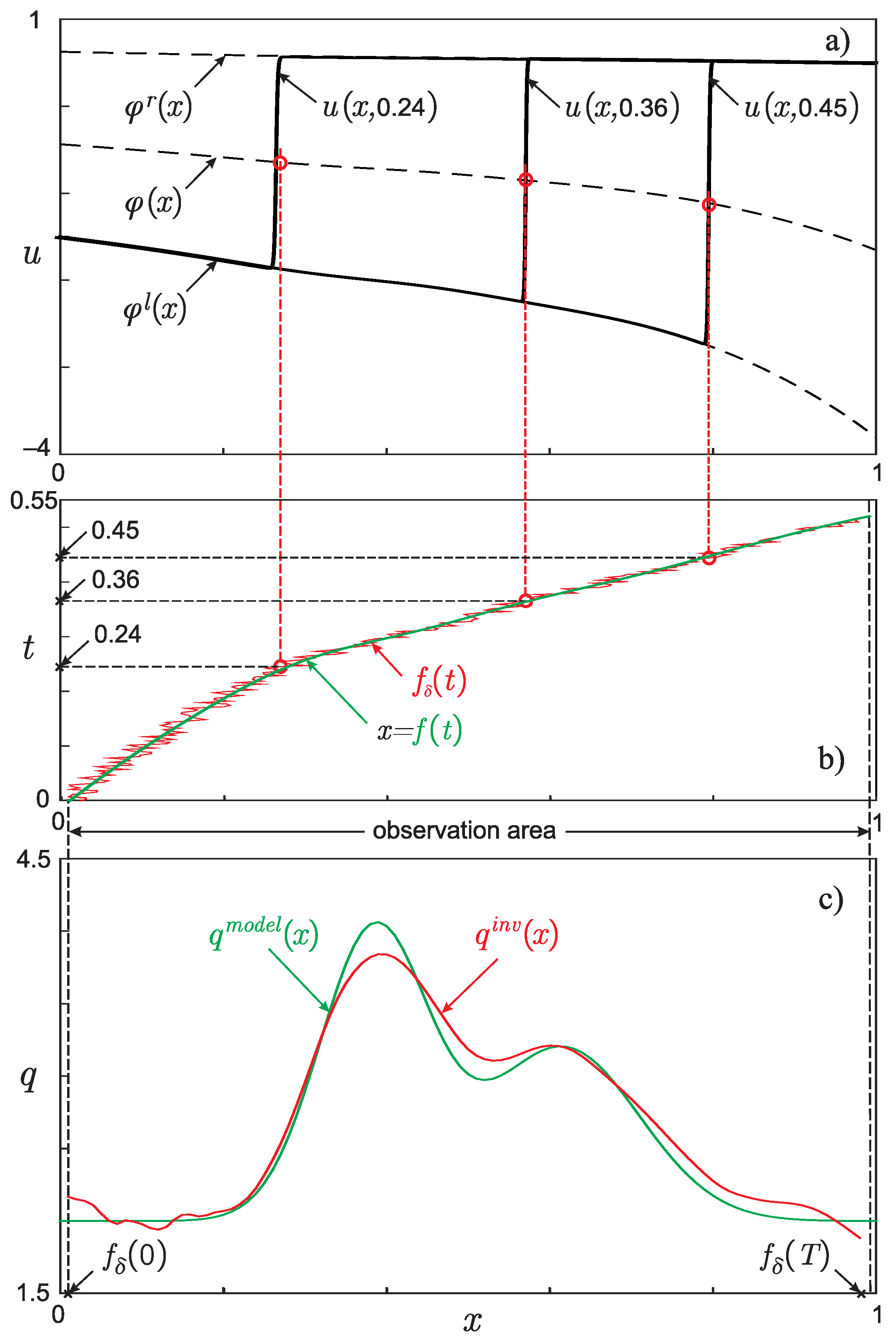
Figure 4 shows the model function f ( t ) and the result of restoring the function q i n v ( x ) from the simulated data f δ ( t ) , given with an error. When implementing the proposed algorithm grids with N = 100 and M = 200 intervals were used. In this case, k m i n = 1 and k m a x = 98 . As a result, the real recovery of the function occurs on the segment x [ 0.01 , 0.098 ] , which is reflected in the figure.
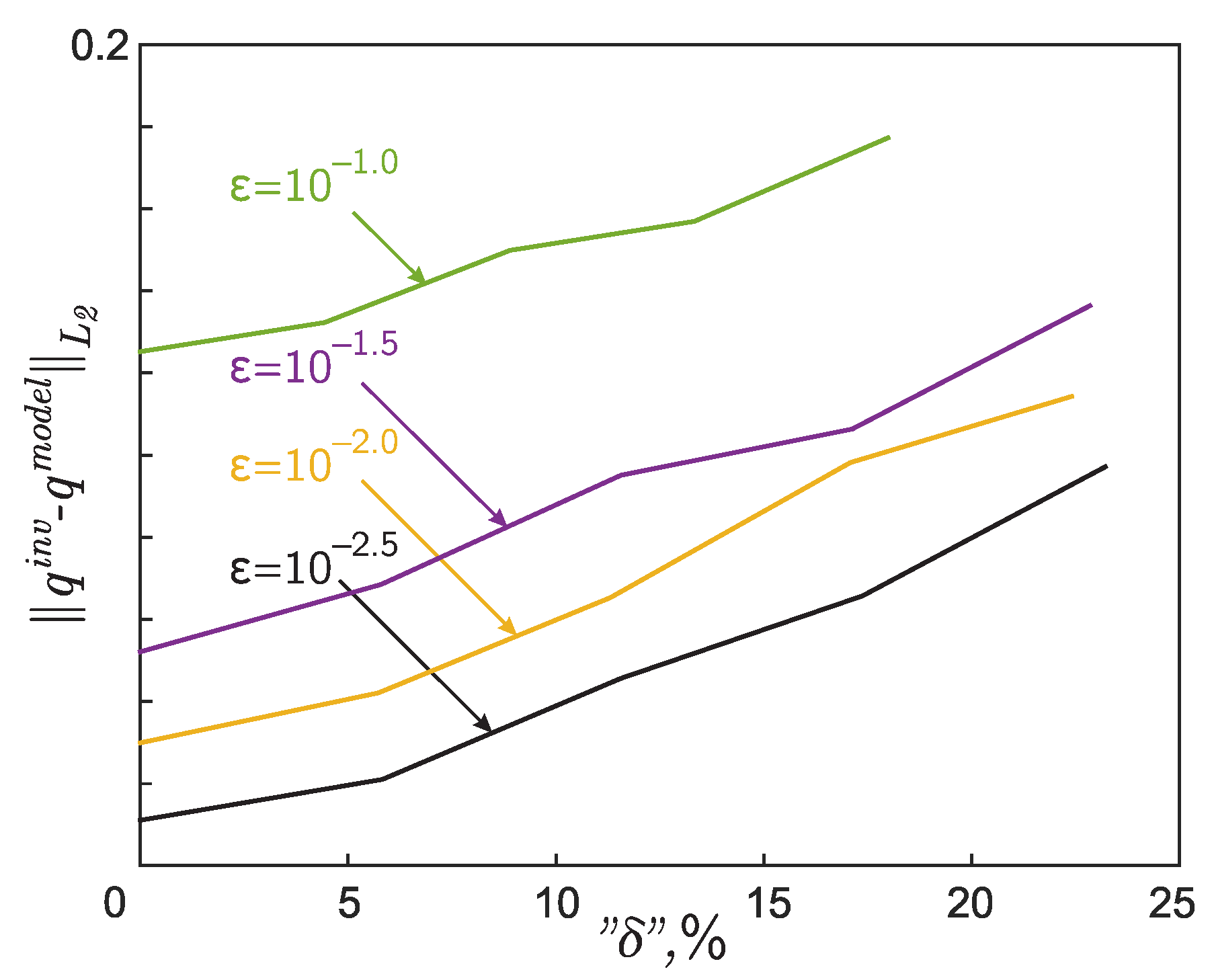
Figure 5 shows the dependence q i n v ( x ) q m o d e l ( x ) L 2 ( [ f ( 0 ) , f ( T ) ] ) on the error level of the input data “ δ = δ / < f δ ( t ) L 2 ( [ 0 , T ] ) > · 100 % in percents, where < · > means averaging over the performed set of experiments (10 experiments) for the same δ . Thus, we have numerically shown that (1) small values of the parameter ε correspond to a more accurate reconstruction of the unknown function q ( x ) , (2) the inverse problem solution is stable with respect to the input data error level δ .
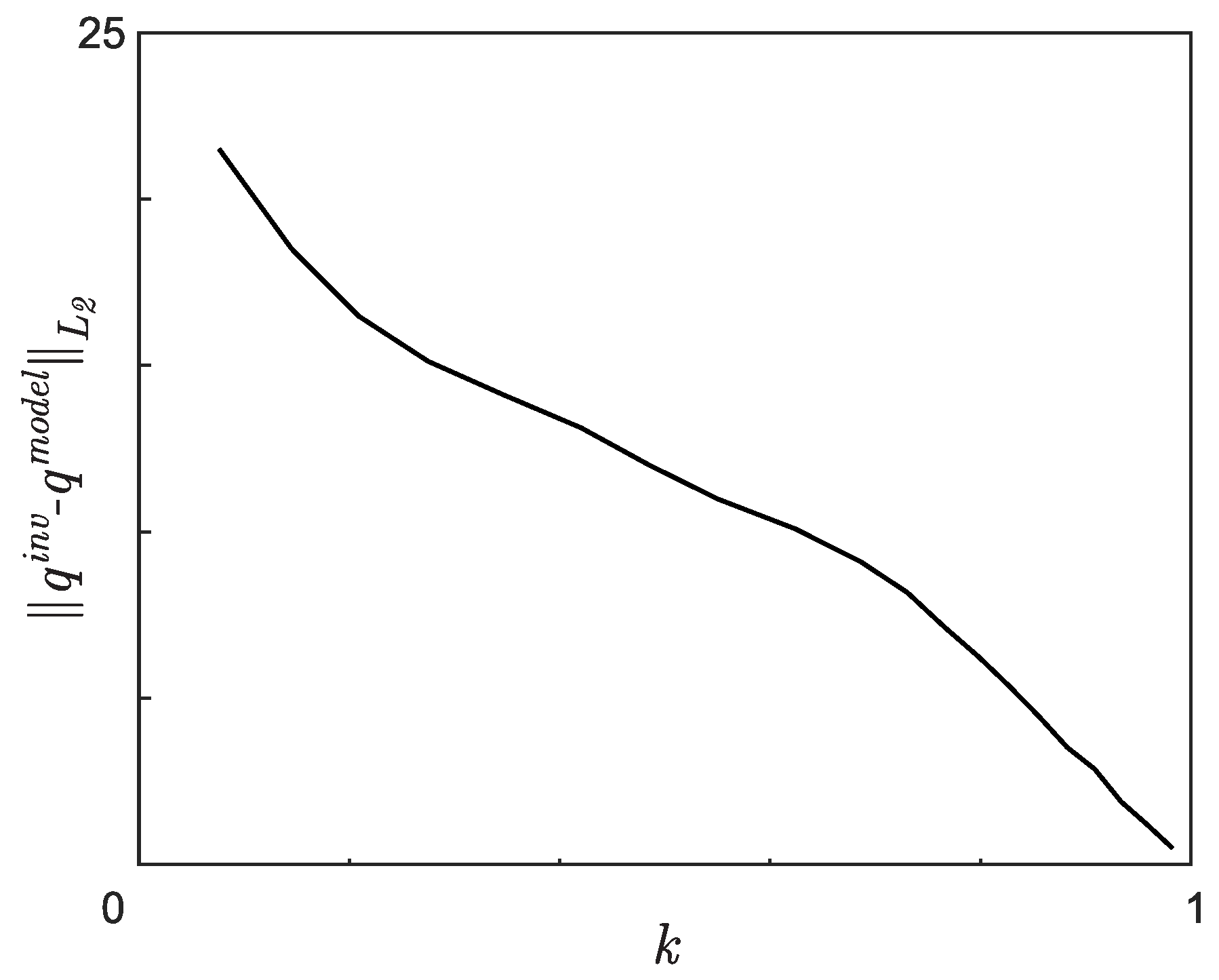
Figure 6 shows the dependence q i n v ( x ) q m o d e l ( x ) L 2 ( [ f ( 0 ) , f ( T ) ] ) on k, where k = ( f δ ( T ) f δ ( 0 ) ) / ( 1 0 ) denoting the part of the region [ 0 , 1 ] that the reaction front passes through during the observation time T. Thus, we have numerically shown that the quality of solution reconstruction strongly depends on the size of the domain in the spatial variable x which the reaction front passed through during its experimental observation. It can be expected that the unknown function q ( x ) will be restored in the best way at k 1 .

6. Conclusions

One of the main result of the paper is using the method of asymptotic analysis in order to obtain mathematical connection between the unknown coefficient and the data of the inverse problem. The second result is the algorithm of solving obtained nonlinear integral equation. It has been shown that the above-proposed algorithm gives good results if (1) the reaction front has passed most of the region in terms of the spatial variable during its experimental observation, and (2) the parameter ε , included in the original problem statement, is sufficiently small. If the size of the observation area is not large enough, the obtained solution can be used as a good initial approximation when solving the inverse problem in the full statement (see, for example, [38]). Some recent results concerning features of solving nonlinear inverse problems (see, for example, [47,48,49,50,51,52,53,54,55]), could be used to construct more efficient algorithms, including error estimation (see, for example, [56,57,58,59,60,61,62]).

Author Contributions

Conceptualization, D.L.; methodology, D.L., N.L., R.A. and A.G.; software, A.G. and R.A.; validation, A.G. and R.A.; formal analysis, D.L. and N.L.; investigation, D.L., N.L., A.G. and R.A.; resources, A.G.; data curation, R.A.; writing—original draft preparation, D.L.; writing—review and editing, D.L.; visualization, D.L., A.G. and R.A.; supervision, D.L.; project administration, D.L.; funding acquisition, D.L. All authors have read and agreed to the published version of the manuscript.

Funding

The reported study was funded by RFBR, project number 20-31-70016.

Institutional Review Board Statement

Not applicable.

Informed Consent Statement

Not applicable.

Conflicts of Interest

The authors declare no conflict of interest.

References

  1. Danilov, V.; Maslov, V.; Volosov, K. Mathematical Modelling of Heat and Mass Transfer Processes; Kluwer: Dordrecht, The Netherlands, 1995. [Google Scholar]
  2. Zeldovich, Y.; Barenblatt, G.; Librovich, V.; Makhviladze, G. The Mathematical Theory of Combustion and Explosions; Plenum: New York, NY, USA, 1985. [Google Scholar]
  3. Butuzov, V.; Vasil’eva, A. Singularly perturbed problems with boundary and interior layers: Theory and applications. Adv. Chem. Phys. 1997, 97, 47–179. [Google Scholar]
  4. Liu, Z.; Liu, Q.; Lin, H.C.; Schwartz, C.; Lee, Y.H.; Wang, T. Three-dimensional variational assimilation of MODIS aerosol optical depth: Implementation and application to a dust storm over East Asia. J. Geophys. Res. Atmos. 2010, 116. [Google Scholar] [CrossRef] [Green Version]
  5. Egger, H.; Fellner, K.; Pietschmann, J.F.; Tang, B.Q. Analysis and numerical solution of coupled volume-surface reaction-diffusion systems with application to cell biology. Appl. Math. Comput. 2018, 336, 351–367. [Google Scholar] [CrossRef] [Green Version]
  6. Yaparova, N. Method for determining particle growth dynamics in a two-component alloy. Steel Transl. 2020, 50, 95–99. [Google Scholar] [CrossRef]
  7. Lin, G.; Zhang, Y.; Cheng, X.; Gulliksson, M.; Forssén, P.; Fornstedt, T. A regularizing Kohn–Vogelius formulation for the model-free adsorption isotherm estimation problem in chromatography. Appl. Anal. 2018, 97, 13–40. [Google Scholar] [CrossRef]
  8. Wu, X.; Ni, M. Existence and stability of periodic contrast structure in reaction-advection-diffusion equation with discontinuous reactive and convective terms. Commun. Nonlinear Sci. Numer. Simul. 2020, 91, 105457. [Google Scholar] [CrossRef]
  9. Zhang, Y.; Lin, G.; Gulliksson, M.; Forssén, P.; Fornstedt, T.; Cheng, X. An adjoint method in inverse problems of chromatography. Inverse Probl. Sci. Eng. 2017, 25, 1112–1137. [Google Scholar] [CrossRef]
  10. Davydova, M.; Zakharova, S. Multidimensional thermal structures in the singularly perturbed stationary models of heat and mass transfer with a nonlinear coefficient of thermal conductivity. J. Comput. Appl. Math. 2021, 400, 113731. [Google Scholar] [CrossRef]
  11. Volpert, A.; Volpert, V.; Volpert, V. Traveling Wave Solutions of Parabolic Systems; American Mathematical Society: Providence, RI, USA, 2000. [Google Scholar]
  12. Meinhardt, H. Models of Biological Pattern Formation; Academic Press: London, UK, 1982. [Google Scholar]
  13. FitzHugh, R. Impulses and physiological states in theoretical model of nerve membrane. Biophys. J. 1961, 1, 445–466. [Google Scholar] [CrossRef] [Green Version]
  14. Murray, J. Mathematical Biology. I. An Introduction; Springer: New York, NY, USA, 2002. [Google Scholar] [CrossRef]
  15. Egger, H.; Pietschmann, J.F.; Schlottbom, M. Identification of nonlinear heat conduction laws. J. Inverse Ill-Posed Probl. 2015, 23, 429–437. [Google Scholar] [CrossRef] [Green Version]
  16. Gholami, A.; Mang, A.; Biros, G. An inverse problem formulation for parameter estimation of a reaction-diffusion model of low grade gliomas. J. Math. Biol. 2016, 72, 409–433. [Google Scholar] [CrossRef] [Green Version]
  17. Aliev, R.; Panfilov, A. A simple two-variable model of cardiac excitation. Chaos Solitons Fractals 1996, 7, 293–301. [Google Scholar] [CrossRef]
  18. Generalov, E.; Levashova, N.; Sidorova, A.; Chumankov, P.; Yakovenko, L. An autowave model of the bifurcation behavior of transformed cells in response to polysaccharide. Biophysics 2017, 62, 876–881. [Google Scholar] [CrossRef]
  19. Mang, A.; Gholami, A.; Davatzikos, C.; Biros, G. PDE-constrained optimization in medical image analysis. Optim. Eng. 2018, 19, 765–812. [Google Scholar] [CrossRef] [Green Version]
  20. Kabanikhin, S.; Shishlenin, M. Recovering a Time-Dependent Diffusion Coefficient from Nonlocal Data. Numer. Anal. Appl. 2018, 11, 38–44. [Google Scholar] [CrossRef]
  21. Mamkin, V.; Kurbatova, J.; Avilov, V.; Mukhartova, Y.; Krupenko, A.; Ivanov, D.; Levashova, N.; Olchev, A. Changes in net ecosystem exchange of CO2, latent and sensible heat fluxes in a recently clear-cut spruce forest in western Russia: Results from an experimental and modeling analysis. Environ. Res. Lett. 2016, 11, 125012. [Google Scholar] [CrossRef]
  22. Levashova, N.; Sidorova, A.; Semina, A.; Ni, M. A spatio-temporal autowave model of shanghai territory development. Sustainability 2019, 11, 3658. [Google Scholar] [CrossRef] [Green Version]
  23. Penenko, A.V.; Mukatova, Z.; Blem, A. Numerical solution of the inverse source problems for the advection-diffusion-reaction models with image-type measurement data. AIP Conf. Proc. 2018, 2027, 030106. [Google Scholar]
  24. Penenko, A. Convergence analysis of the adjoint ensemble method in inverse source problems for advection-diffusion-reaction models with image-type measurements. Inverse Probl. Imaging 2018, 14, 757782. [Google Scholar]
  25. Zakharova, S.; Davydova, M.; Lukyanenko, D. Use of asymptotic analysis for solving the inverse problem of source parameters determination of nitrogen oxide emission in the atmosphere. Inverse Probl. Sci. Eng. 2021, 29, 365–377. [Google Scholar] [CrossRef]
  26. Isakov, V.; Kabanikhin, S.; Shananin, A.; Shishlenin, M.; Zhang, S. Algorithm for determining the volatility function in the Black-Scholes model. Comput. Math. Math. Phys. 2019, 59, 1753–1758. [Google Scholar] [CrossRef]
  27. Kadalbajoo, M.; Gupta, V. A brief survey on numerical methods for solving singularly perturbed problems. Appl. Math. Comput. 2010, 217, 3641–3716. [Google Scholar] [CrossRef]
  28. Cannon, J.; DuChateau, P. An Inverse problem for a nonlinear diffusion equation. SIAM J. Appl. Math. 1980, 39, 272–289. [Google Scholar] [CrossRef]
  29. DuChateau, P.; Rundell, W. Unicity in an inverse problem for an unknown reaction term in a reaction-diffusion equation. J. Differ. Equ. 1985, 59, 155–164. [Google Scholar] [CrossRef] [Green Version]
  30. Pilant, M.; Rundell, W. An inverse problem for a nonlinear parabolic equation. Commun. Partial. Differ. Equ. 1986, 11, 445–457. [Google Scholar] [CrossRef]
  31. Kabanikhin, S. Definitions and examples of inverse and ill-posed problems. J. Inverse Ill-Posed Probl. 2008, 16, 317–357. [Google Scholar] [CrossRef]
  32. Kabanikhin, S. Inverse and Ill-Posed Problems Theory and Applications; de Gruyter: Berlin, Germany, 2011. [Google Scholar]
  33. Jin, B.; Rundell, W. A tutorial on inverse problems for anomalous diffusion processes. Inverse Probl. 2015, 31, 035003. [Google Scholar] [CrossRef] [Green Version]
  34. Belonosov, A.; Shishlenin, M. Regularization methods of the continuation problem for the parabolic equation. Lect. Notes Comput. Sci. 2017, 10187, 220–226. [Google Scholar]
  35. Kaltenbacher, B.; Rundell, W. On the identification of a nonlinear term in a reaction-diffusion equation. Inverse Probl. 2019, 35, 115007. [Google Scholar] [CrossRef] [Green Version]
  36. Belonosov, A.; Shishlenin, M.; Klyuchinskiy, D. A comparative analysis of numerical methods of solving the continuation problem for 1D parabolic equation with the data given on the part of the boundary. Adv. Comput. Math. 2019, 45, 735–755. [Google Scholar] [CrossRef]
  37. Kaltenbacher, B.; Rundell, W. The inverse problem of reconstructing reaction-diffusion systems. Inverse Problems 2020, 36, 065011. [Google Scholar] [CrossRef]
  38. Lukyanenko, D.; Yeleskina, T.; Prigorniy, I.; Isaev, T.; Borzunov, A.; Shishlenin, M. Inverse problem of recovering the initial condition for a nonlinear equation of the reaction-diffusion-advection type by data given on the position of a reaction front with a time delay. Mathematics 2021, 9, 342. [Google Scholar] [CrossRef]
  39. Lukyanenko, D.; Borzunov, A.; Shishlenin, M. Solving coefficient inverse problems for nonlinear singularly perturbed equations of the reaction-diffusion-advection type with data on the position of a reaction front. Commun. Nonlinear Sci. Numer. Simul. 2021, 99, 105824. [Google Scholar] [CrossRef]
  40. Levashova, N.; Gorbachev, A.; Argun, R.; Lukyanenko, D. The problem of the non-uniqueness of the solution to the inverse problem of recovering the symmetric states of a bistable medium with data on the position of an autowave front. Symmetry 2021, 13, 680. [Google Scholar] [CrossRef]
  41. Lukyanenko, D.; Shishlenin, M.; Volkov, V. Asymptotic analysis of solving an inverse boundary value problem for a nonlinear singularly perturbed time-periodic reaction-diffusion-advection equation. J. Inverse Ill-Posed Probl. 2019, 27, 745–758. [Google Scholar] [CrossRef]
  42. Rudenko, O.; Hedberg, C. The quadratically cubic Burgers equation: An exactly solvable nonlinear model for shocks, pulses and periodic waves. Nonlinear Dyn. 2016, 85, 767–776. [Google Scholar] [CrossRef] [Green Version]
  43. Vasil’eva, A.; Butuzov, V.; Nefedov, N. Singularly perturbed problems with boundary and internal layers. Proc. Steklov Inst. Math. 2010, 268, 258–273. [Google Scholar] [CrossRef]
  44. Lukyanenko, D.; Grigorev, V.; Volkov, V.; Shishlenin, M. Solving of the coefficient inverse problem for a nonlinear singularly perturbed two-dimensional reaction-diffusion equation with the location of moving front data. Comput. Math. Appl. 2019, 77, 1245–1254. [Google Scholar] [CrossRef]
  45. Antipov, E.; Levashova, N.; Nefedov, N. Asymptotics of the front motion in the reaction-diffusion-advection problem. Comput. Math. Math. Phys. 2014, 54, 1536–1549. [Google Scholar] [CrossRef]
  46. Tikhonov, A.N.; Goncharsky, A.V.; Stepanov, V.V.; Yagola, A.G. Numerical Methods for the Solution of Ill-Posed Problems; Kluwer Academic Publishers: Dordrecht, The Netherlands, 1995. [Google Scholar]
  47. Klibanov, M.; Li, J.; Zhang, W. Convexification for an inverse parabolic problem. Inverse Probl. 2020, 36, 085008. [Google Scholar] [CrossRef]
  48. Klibanov, M.; Nguyen, D.L. Convergence of a series associated with the convexification method for coefficient inverse problems. J. Inverse Ill-Posed Probl. 2020, 29. [Google Scholar] [CrossRef]
  49. Leonov, A. Extra-Optimal Methods for Solving Ill-Posed Problems: Survey of Theory and Examples. Comput. Math. Math. Phys. 2020, 60, 960–986. [Google Scholar] [CrossRef]
  50. Bakushinskii, A.; Kokurin, M.; Kokurin, M. Direct and Converse Theorems for Iterative Methods of Solving Irregular Operator Equations and Finite Difference Methods for Solving Ill-Posed Cauchy Problems. Comput. Math. Math. Phys. 2020, 60, 915–937. [Google Scholar] [CrossRef]
  51. Kokurin, M. A posteriori choice of time-discretization step in finite difference methods for solving ill-posed Cauchy problems in Hilbert space. J. Inverse Ill-Posed Probl. 2021. [Google Scholar] [CrossRef]
  52. Lin, G.; Cheng, X.; Zhang, Y. A parametric level set based collage method for an inverse problem in elliptic partial differential equations. J. Comput. Appl. Math. 2018, 340, 101–121. [Google Scholar] [CrossRef] [Green Version]
  53. Gulliksson, M.; Holmbom, A.; Persson, J.; Zhang, Y. A separating oscillation method of recovering the G-limit in standard and non-standard homogenization problems. Inverse Probl. 2016, 32, 025005. [Google Scholar] [CrossRef]
  54. Egger, H.; Engl, H.; Klibanov, M. Global uniqueness and Holder stability for recovering a nonlinear source term in a parabolic equation. Inverse Probl. 2005, 21, 271–290. [Google Scholar] [CrossRef]
  55. Zhang, Y.; Gong, R. Second order asymptotical regularization methods for inverse problems in partial differential equations. J. Comput. Appl. Math. 2020, 375, 112798. [Google Scholar] [CrossRef] [Green Version]
  56. Yagola, A.; Leonov, A.; Titarenko, V. Data errors and an error estimation for ill-posed problems. Inverse Probl. Eng. 2002, 10, 117–129. [Google Scholar] [CrossRef]
  57. Titarenko, V.; Yagola, A. Error estimation for ill-posed problems on piecewise convex functions and sourcewise represented sets. J. Inverse Ill-Posed Probl. 2008, 16, 625–638. [Google Scholar] [CrossRef]
  58. Leonov, A. Which of inverse problems can have a priori approximate solution accuracy estimates comparable in order with the data accuracy. Numer. Anal. Appl. 2014, 7, 284–292. [Google Scholar] [CrossRef]
  59. Leonov, A. A posteriori accuracy estimations of solutions to ill-posed inverse problems and extra-optimal regularizing algorithms for their solution. Numer. Anal. Appl. 2012, 5, 68–83. [Google Scholar] [CrossRef]
  60. Kokurin, M. Accuracy estimates of regularization methods and conditional well-posedness of nonlinear optimization problems. J. Inverse Ill-Posed Probl. 2018, 26, 789–797. [Google Scholar] [CrossRef]
  61. Kokurin, M. Ill-Posed Nonlinear Optimization Problems and Uniform Accuracy Estimates of Regularization Methods. Numer. Funct. Anal. Optim. 2020, 41, 1887–1900. [Google Scholar] [CrossRef]
  62. Chaikovskii, D.; Zhang, Y. Convergence analysis for forward and inverse problems in singularly perturbed time-dependent reaction-advection-diffusion equations. arXiv 2021, arXiv:2106.15249. [Google Scholar]
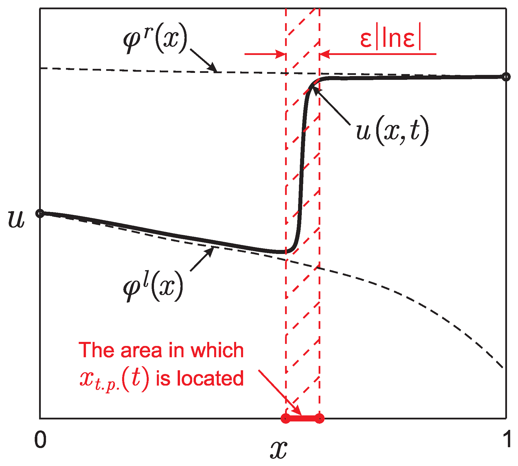
Figure 1. Typical form of the moving front-type solution in Problem (1) for a fixed t. The figure is drawn for set of parameters (16) and time t 0.36 .
Mathematics 09 02342 g001
Figure 2. Relationship of the functions U 0 ( ) ( x , t ) and φ ( x ) with the localization point of the reaction front x t . p . ( t ) .
Mathematics 09 02342 g002
Figure 3. The region passed through by the reaction front during the experimental observations of the function f δ ( t ) x t . p . ( t ) .
Mathematics 09 02342 g003
Figure 4. (a) Solution of the problem (1) at several fixed moments of time t; (b) exact model function f ( t ) and noisy function f δ ( t ) ; (c) result of recovering the function q i n v ( x ) for δ = 0.014 .
Mathematics 09 02342 g004
Figure 5. The norm of the residual versus the noise level δ of the inverse problem data for various ε .
Mathematics 09 02342 g005
Figure 6. Dependence of the accuracy of reconstruction the approximate solution q i n v ( x ) on the part of the region k passed through by the reaction front during its experimental observations (the case of ε = 10 2.5 , δ = 0 ).
Mathematics 09 02342 g006
Publisher’s Note: MDPI stays neutral with regard to jurisdictional claims in published maps and institutional affiliations.