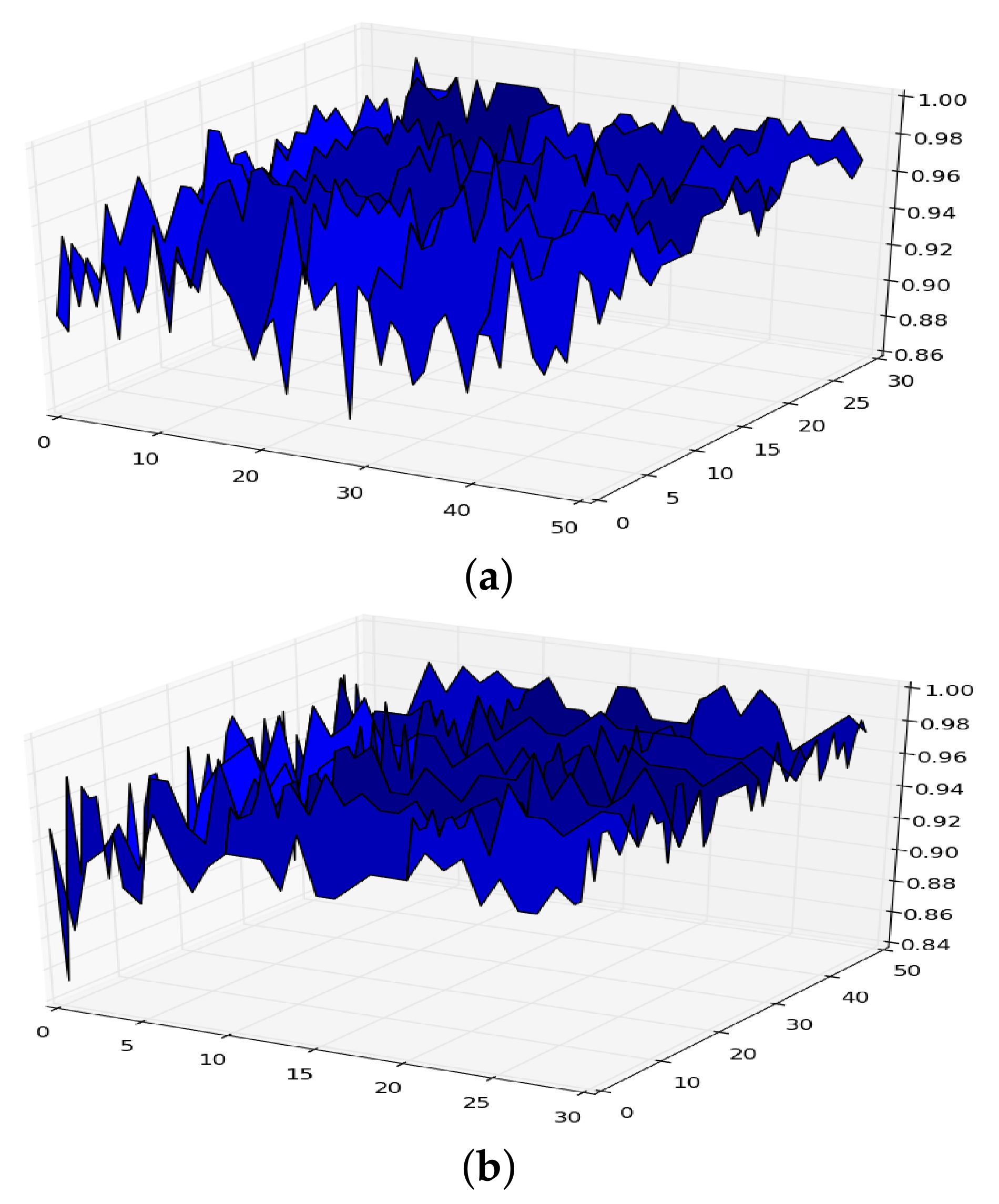
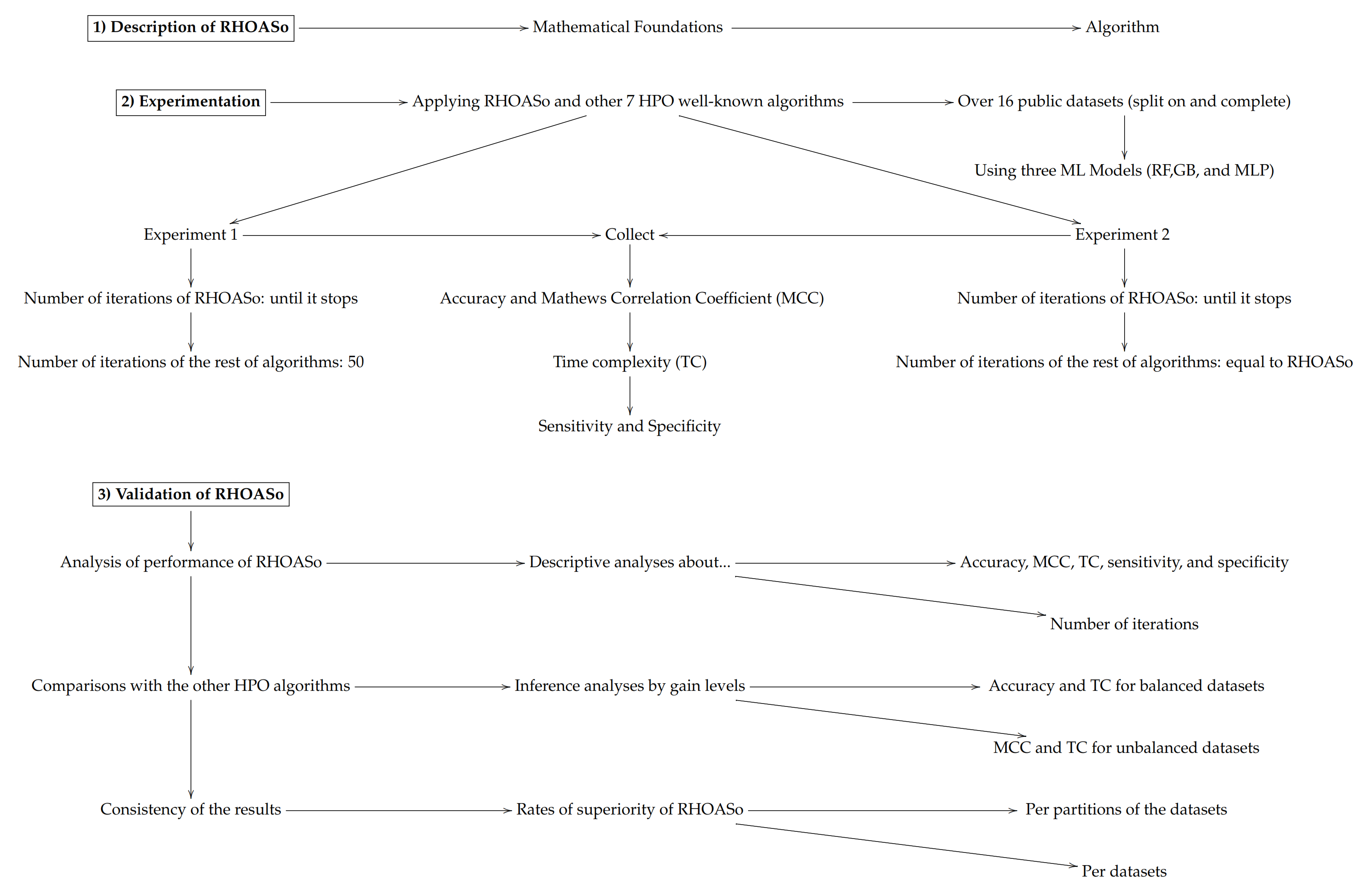
Figure 1.
Surface of for random forest. (a) in RF. (b) in RF.
Figure 1.
Surface of for random forest. (a) in RF. (b) in RF.
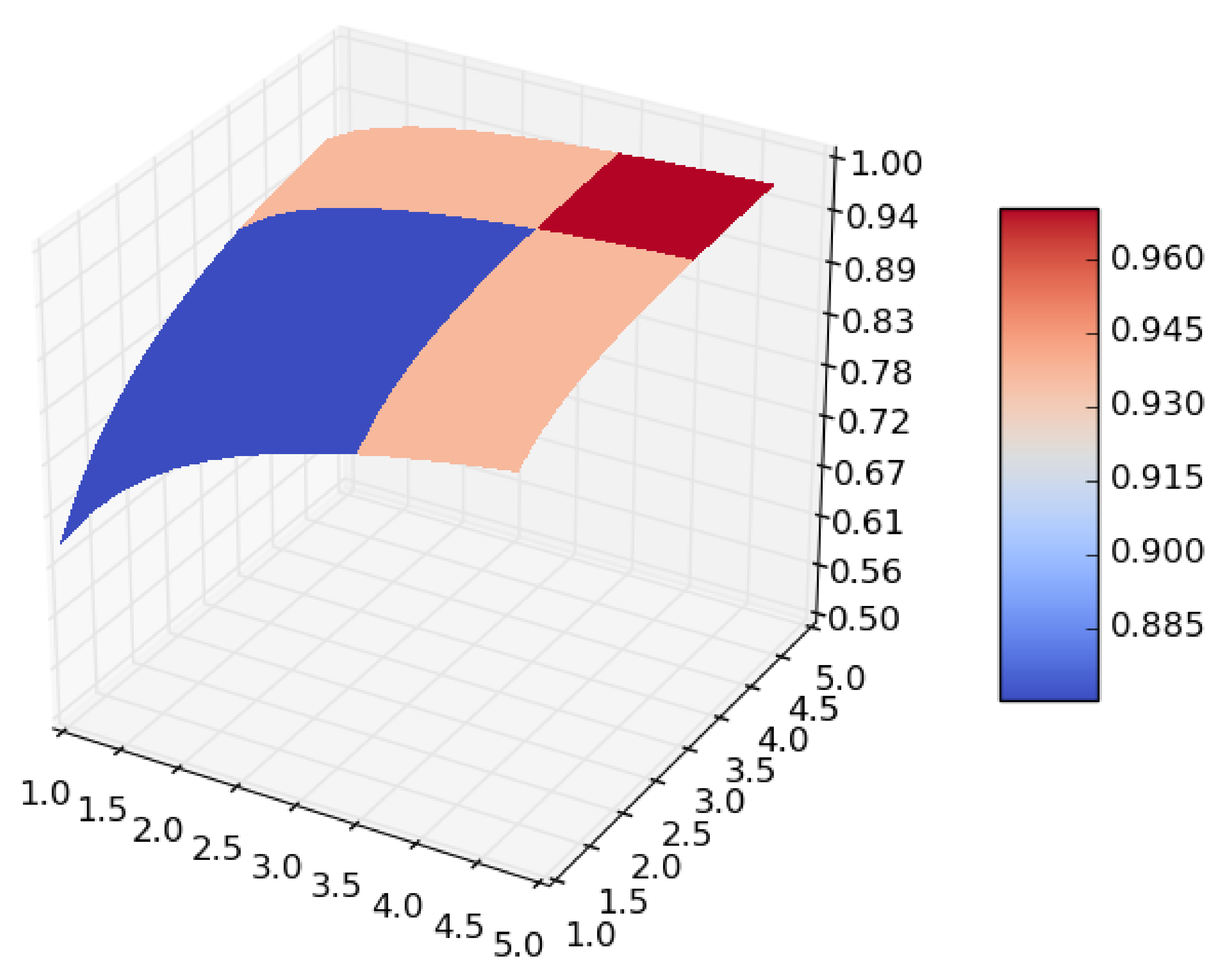
Figure 2.
Smoothing of .
Figure 2.
Smoothing of .
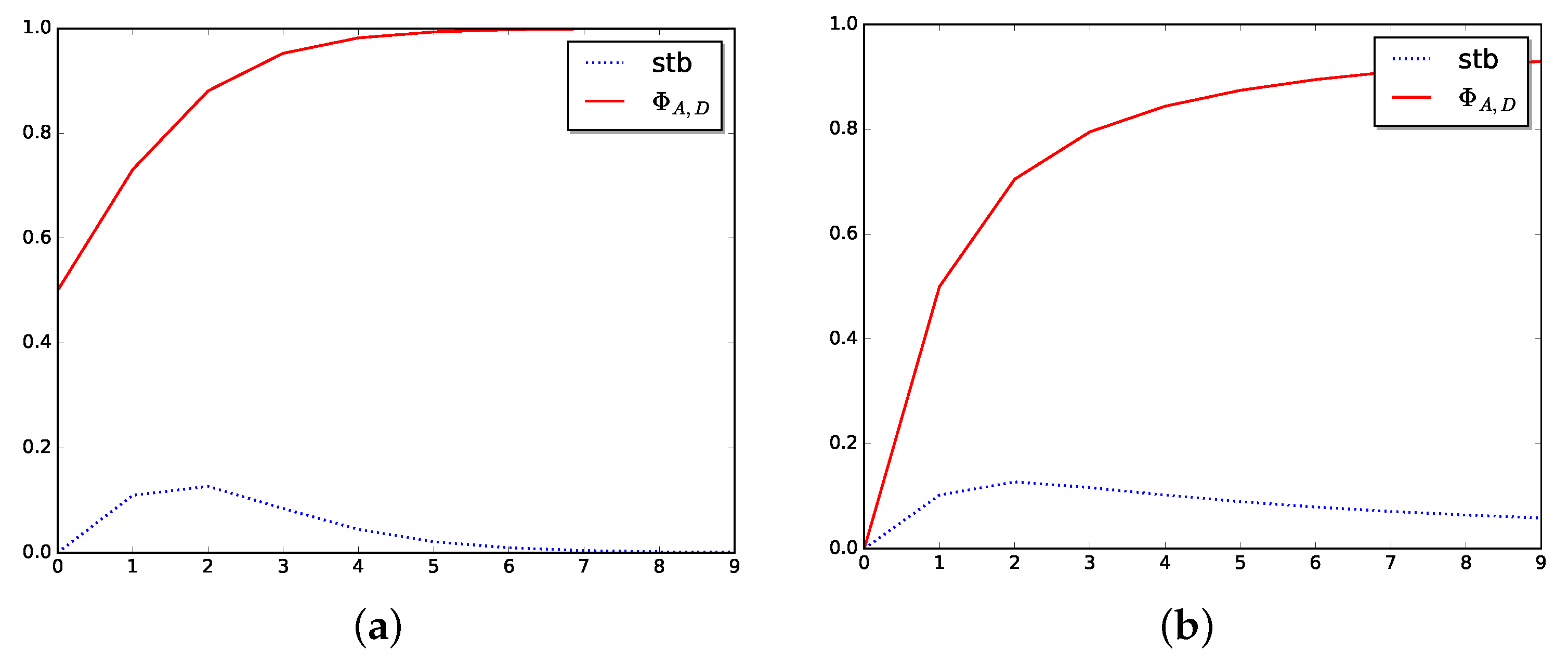
Figure 3.
Stabilizer in dimension one. (a) Stabilizer for logistic function. (b) Stabilizer for arctangent function.
Figure 3.
Stabilizer in dimension one. (a) Stabilizer for logistic function. (b) Stabilizer for arctangent function.
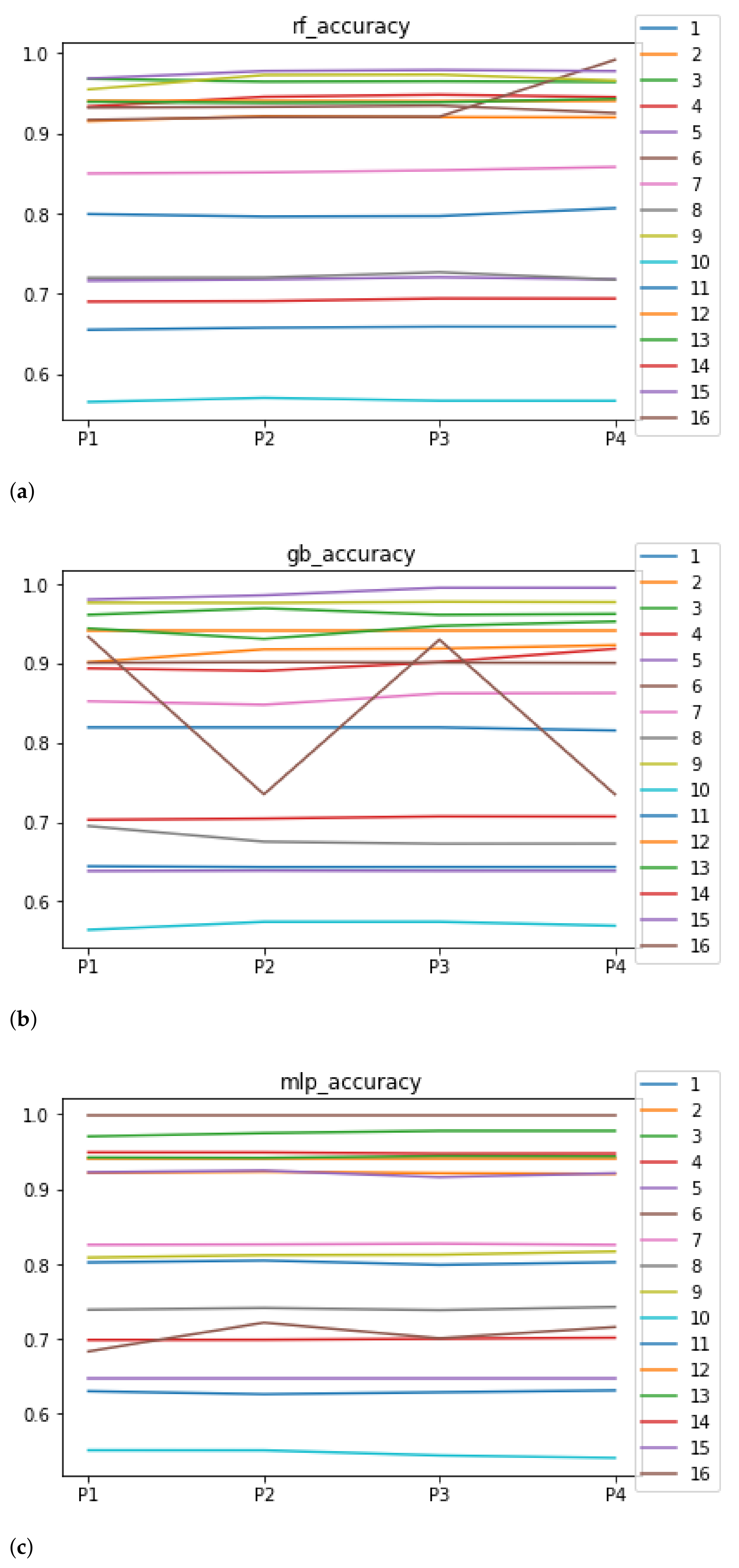
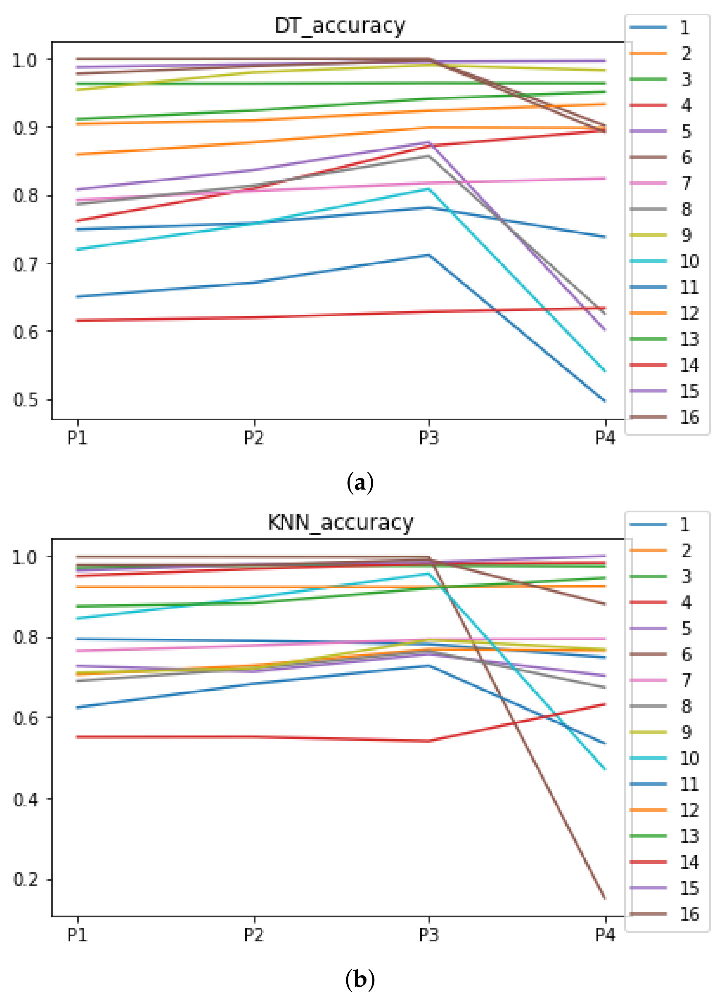
Figure 4.
Behavior of RHOASo: accuracy. Each line represents a dataset. (a) Accuracy for RF. Axis X: the partition of the dataset. Axis Y: the obtained accuracy. (b) Accuracy for GB. Axis X: the partition of the dataset. Axis Y: the obtained accuracy. (c) Accuracy for MLP. Axis X: the partition of the dataset. Axis Y: the obtained accuracy.
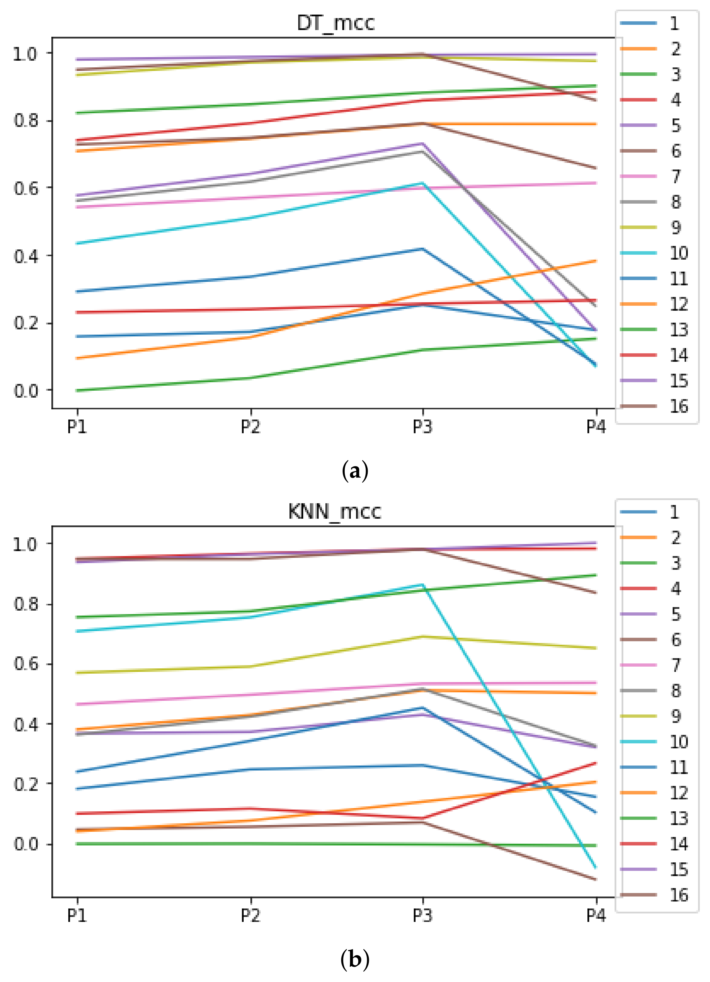
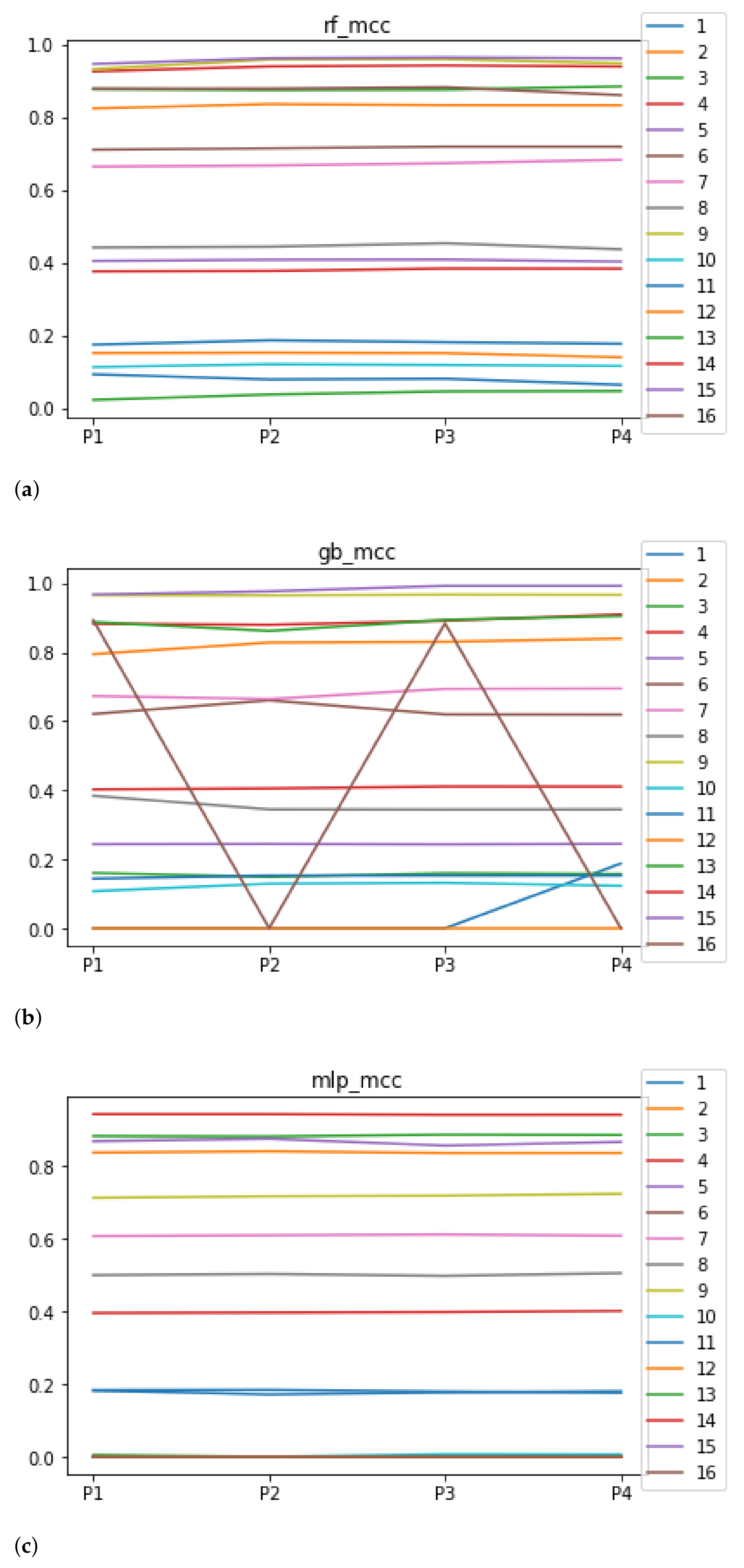
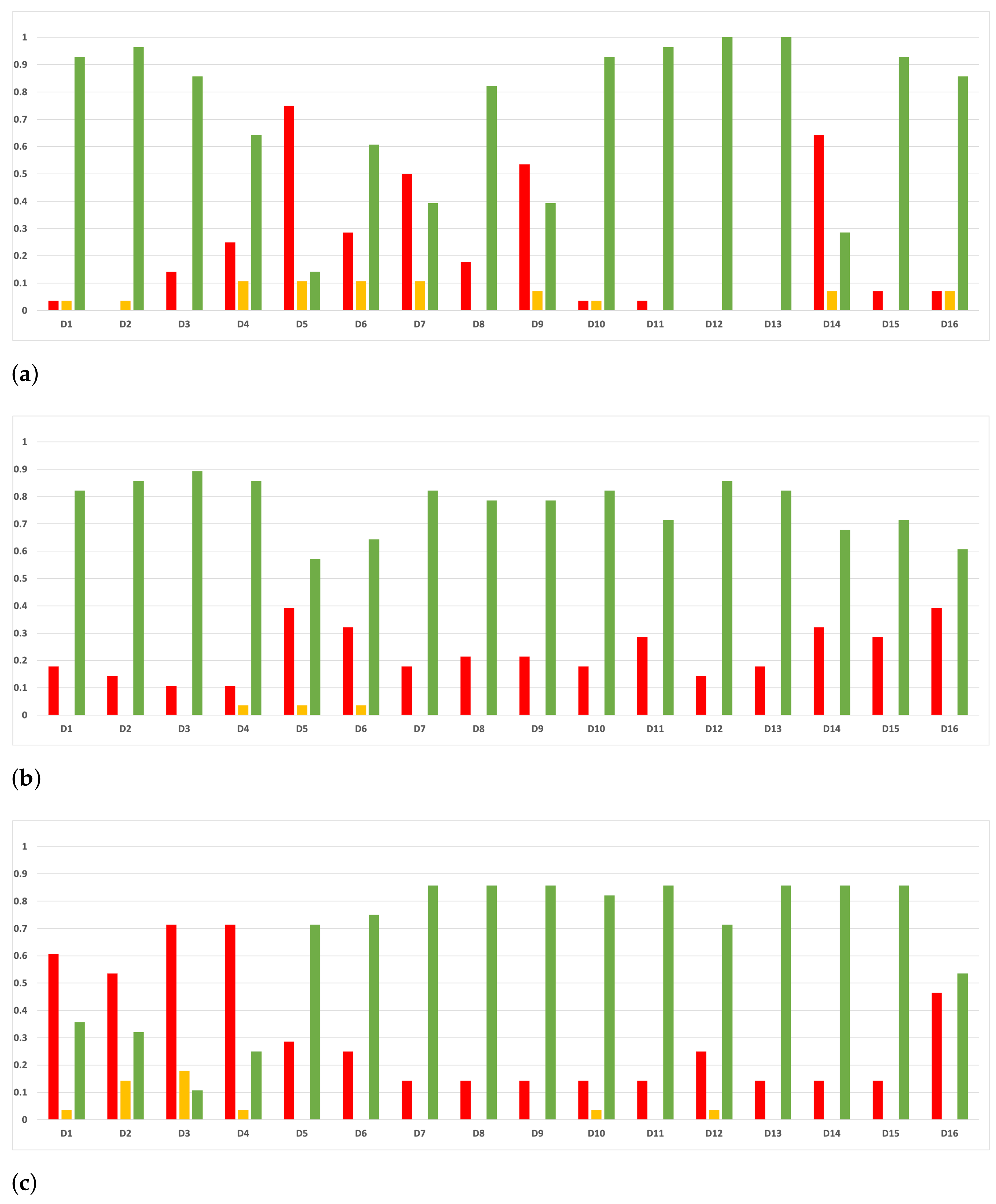
Figure 5.
Behavior of RHOASo: MCC. Each line represents a dataset. (a) MCC for RF. Axis X: the partition of the dataset. Axis Y: the obtained MCC. (b) MCC for GB. Axis X: the partition of the dataset. Axis Y: the obtained MCC. (c) MCC for MLP. Axis X: the partition of the dataset. Axis Y: the obtained MCC.
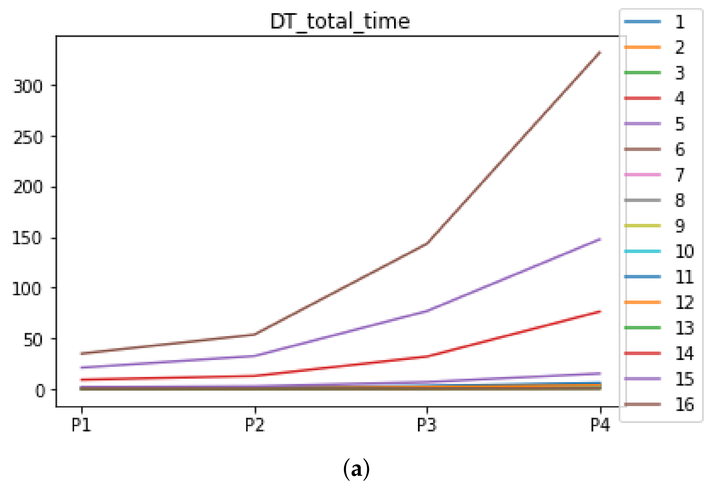
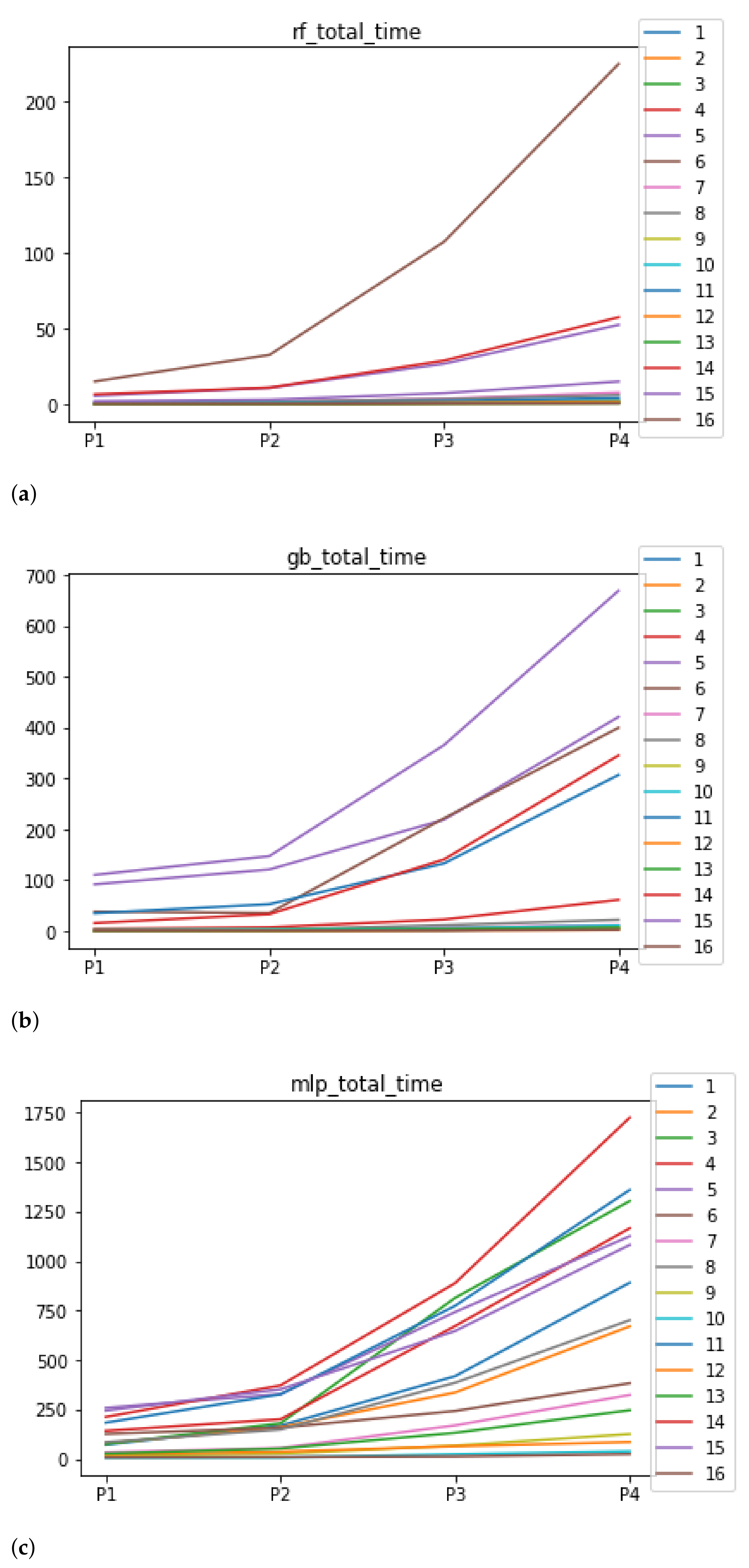
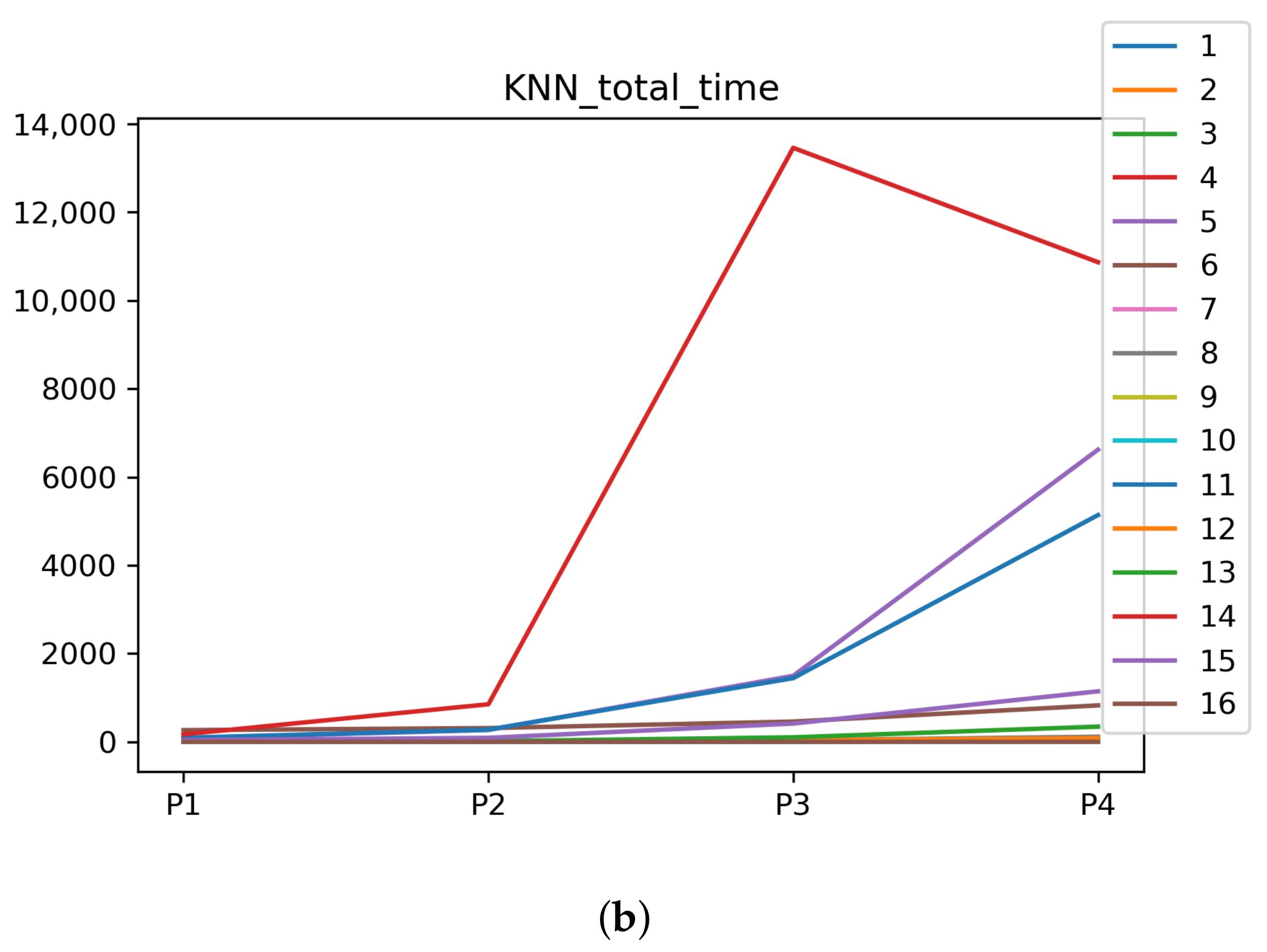
Figure 6.
Behavior of RHOASo: time complexity. Each line represents a dataset. (a) Time complexity for RF. Axis X: the partition of the dataset. Axis Y: the obtained time complexity in seconds. (b) Time complexity for GB. Axis X: the partition of the dataset. Axis Y: the obtained time complexity in seconds. (c) Time complexity for MLP. Axis X: the partition of the dataset. Axis Y: the obtained time complexity in seconds.
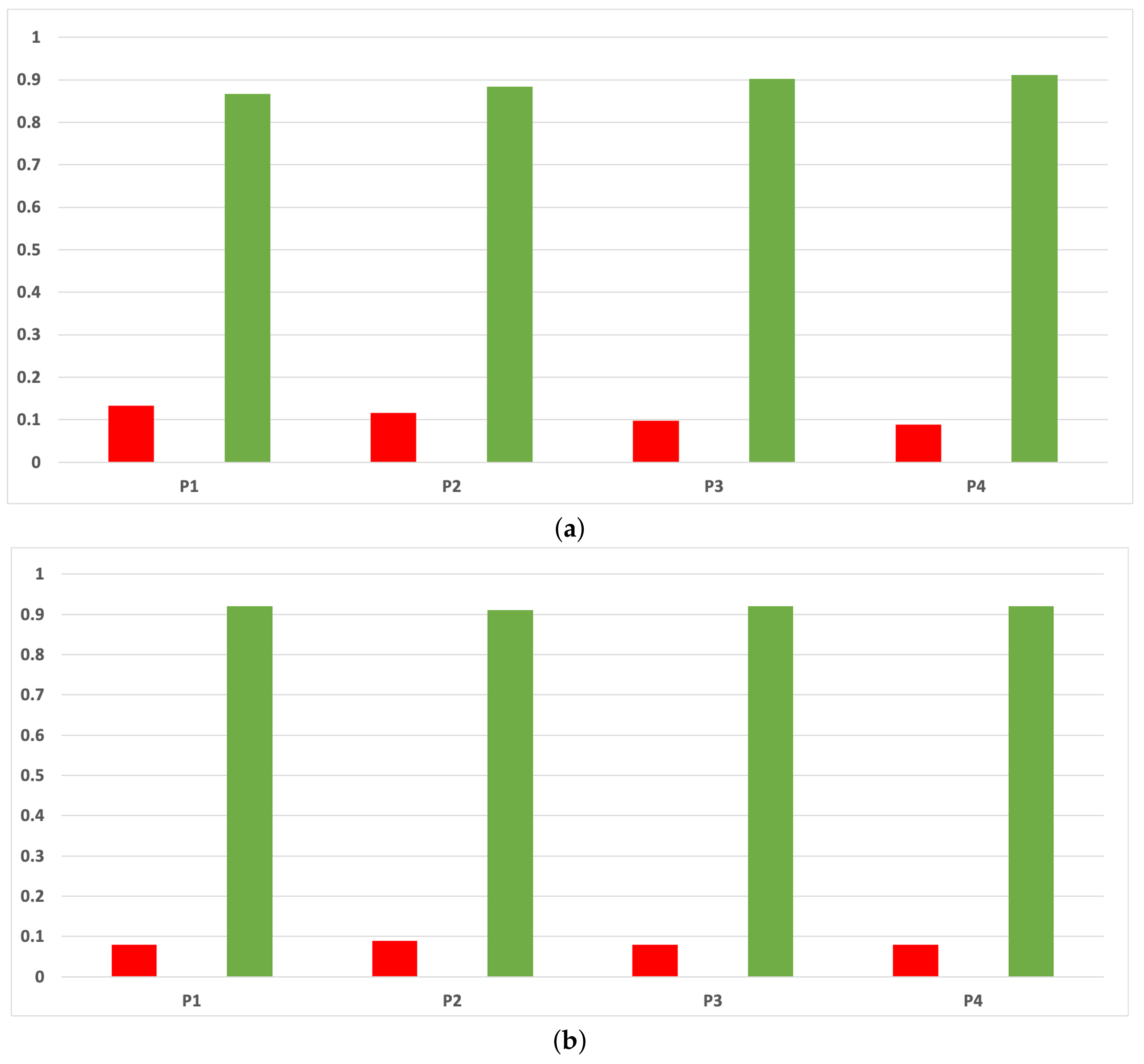
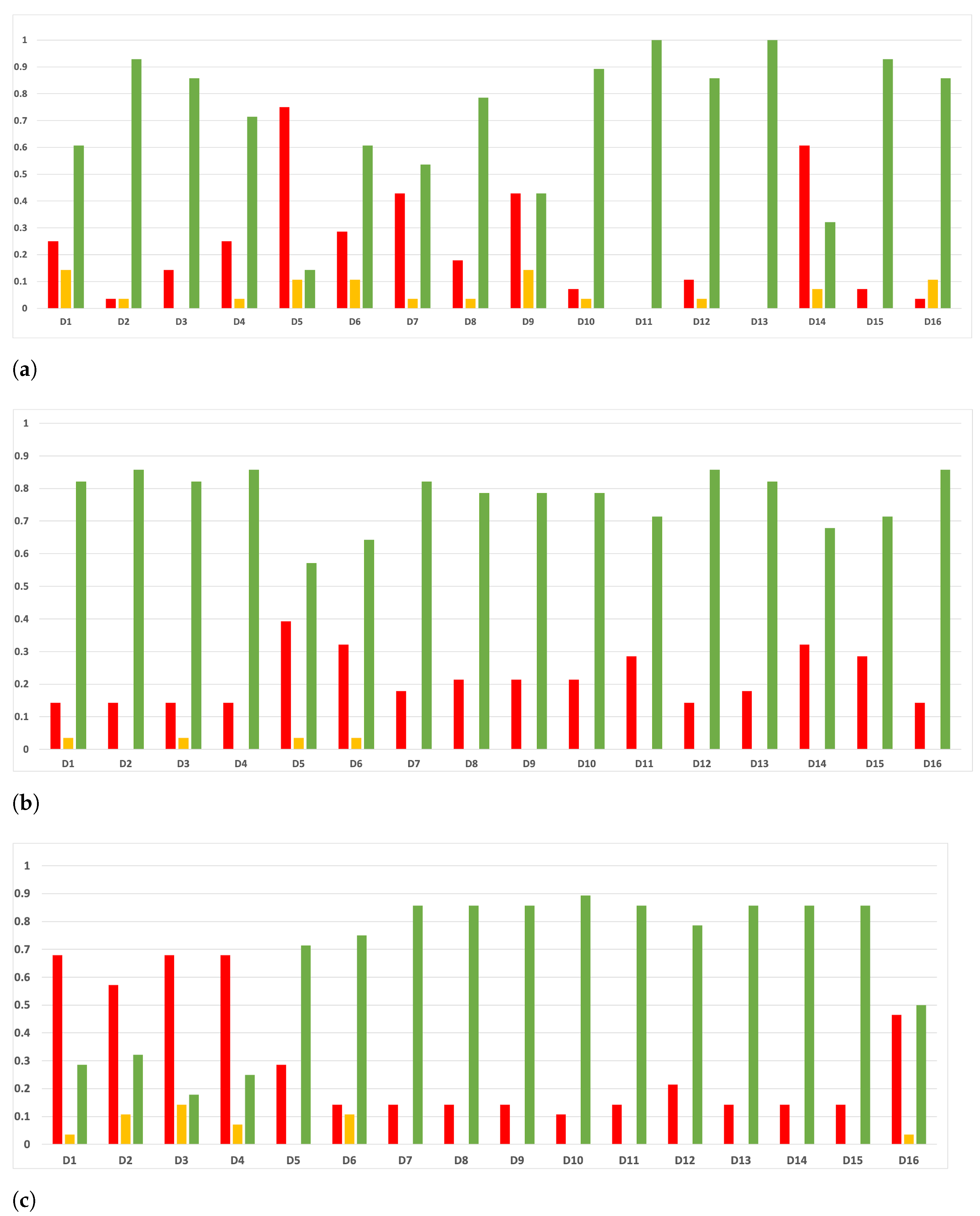
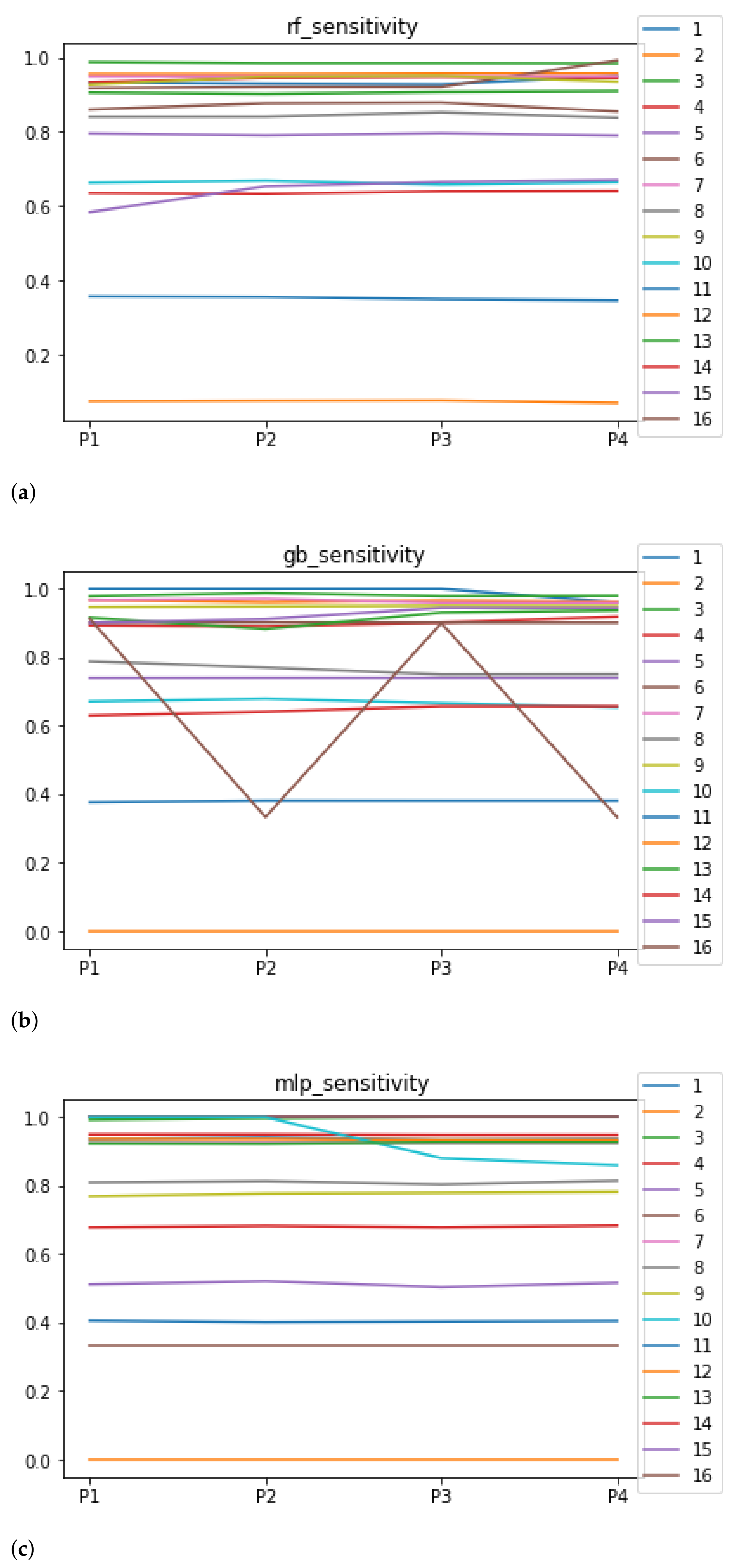
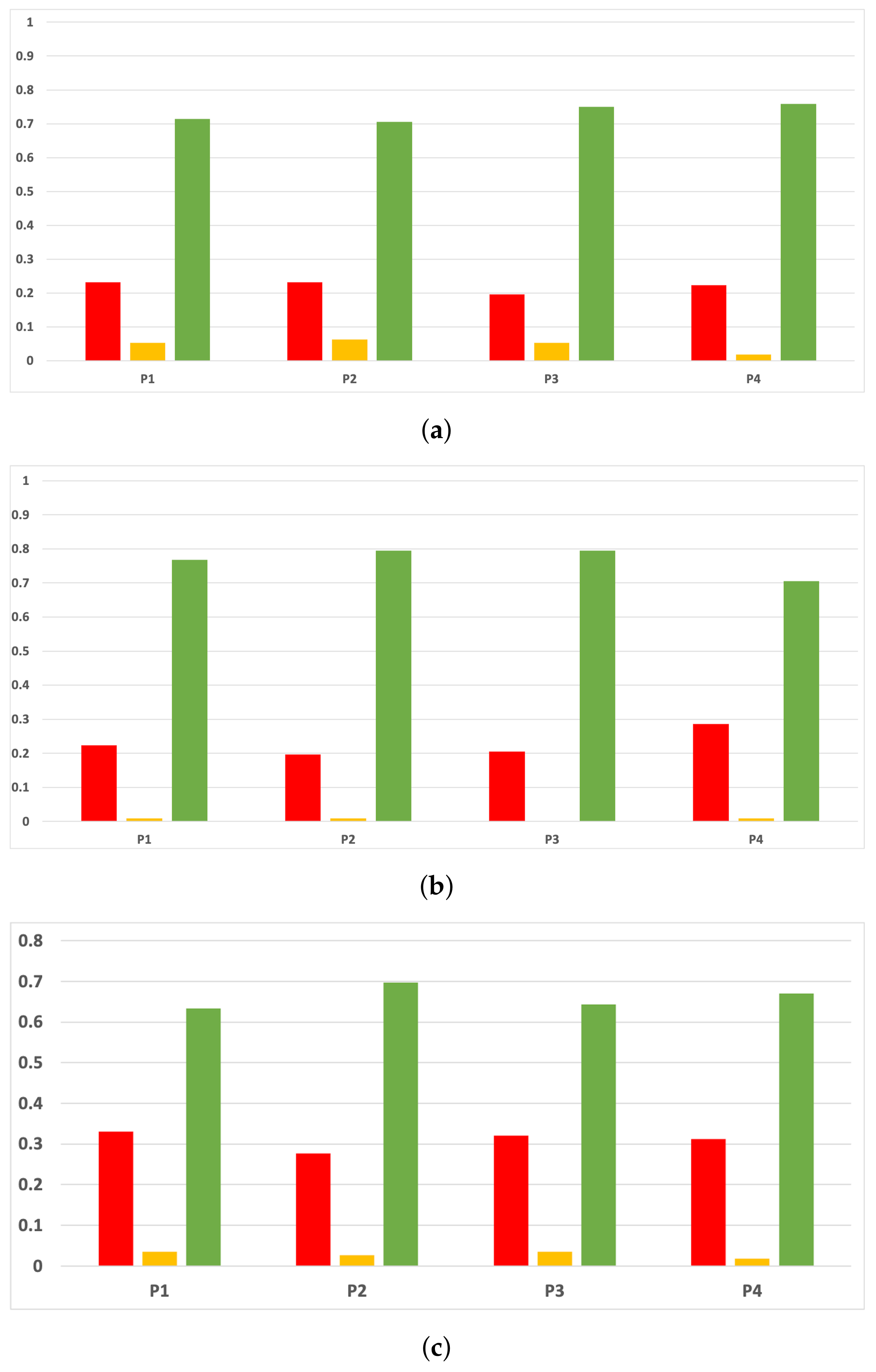
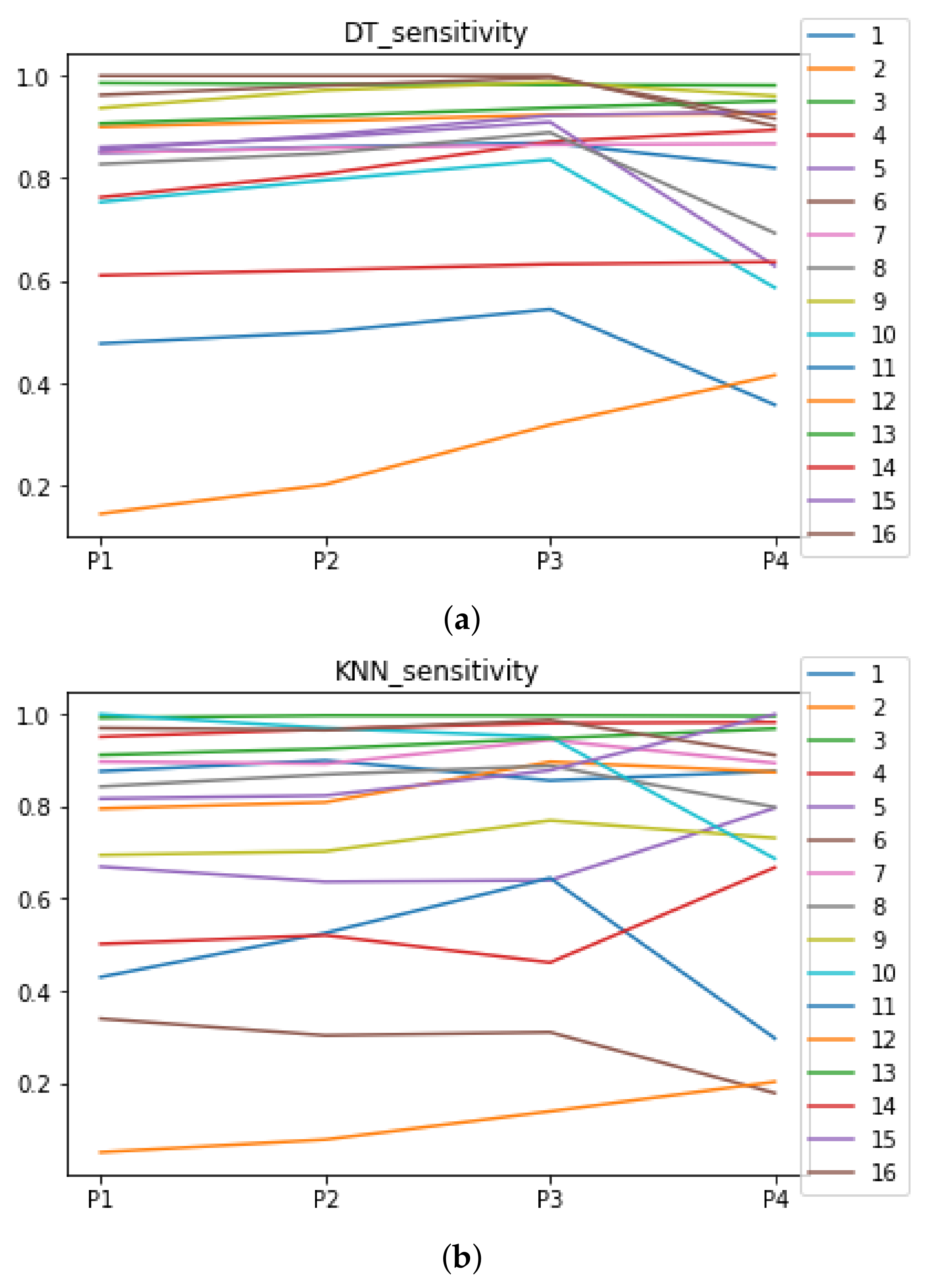
Figure 7.
Behavior RHOASo: sensitivity. The datasets are represented with a bar chart for each partition. (a) Sensitivity for RF. Axis X: the partition of the dataset. Axis Y: the obtained sensitivity. (b) Sensitivity for GB. Axis X: the partition of the dataset. Axis Y: the obtained sensitivity. (c) Sensitivity for MLP. Axis X: the partition of the dataset. Axis Y: the obtained sensitivity.
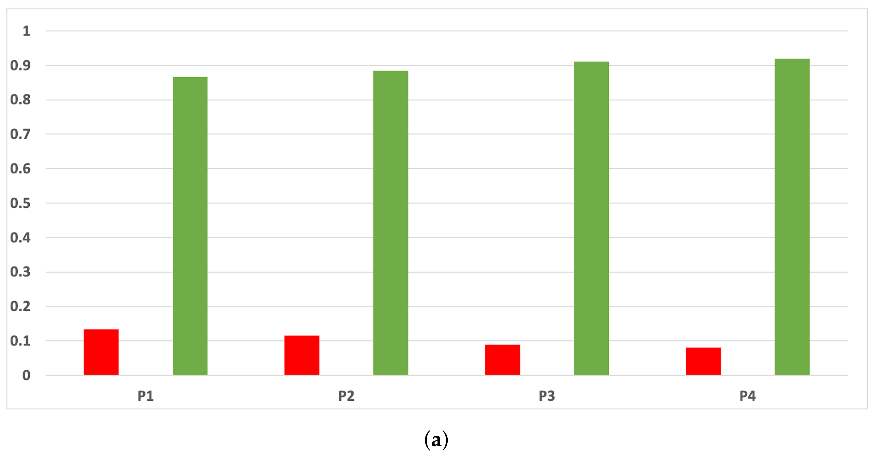
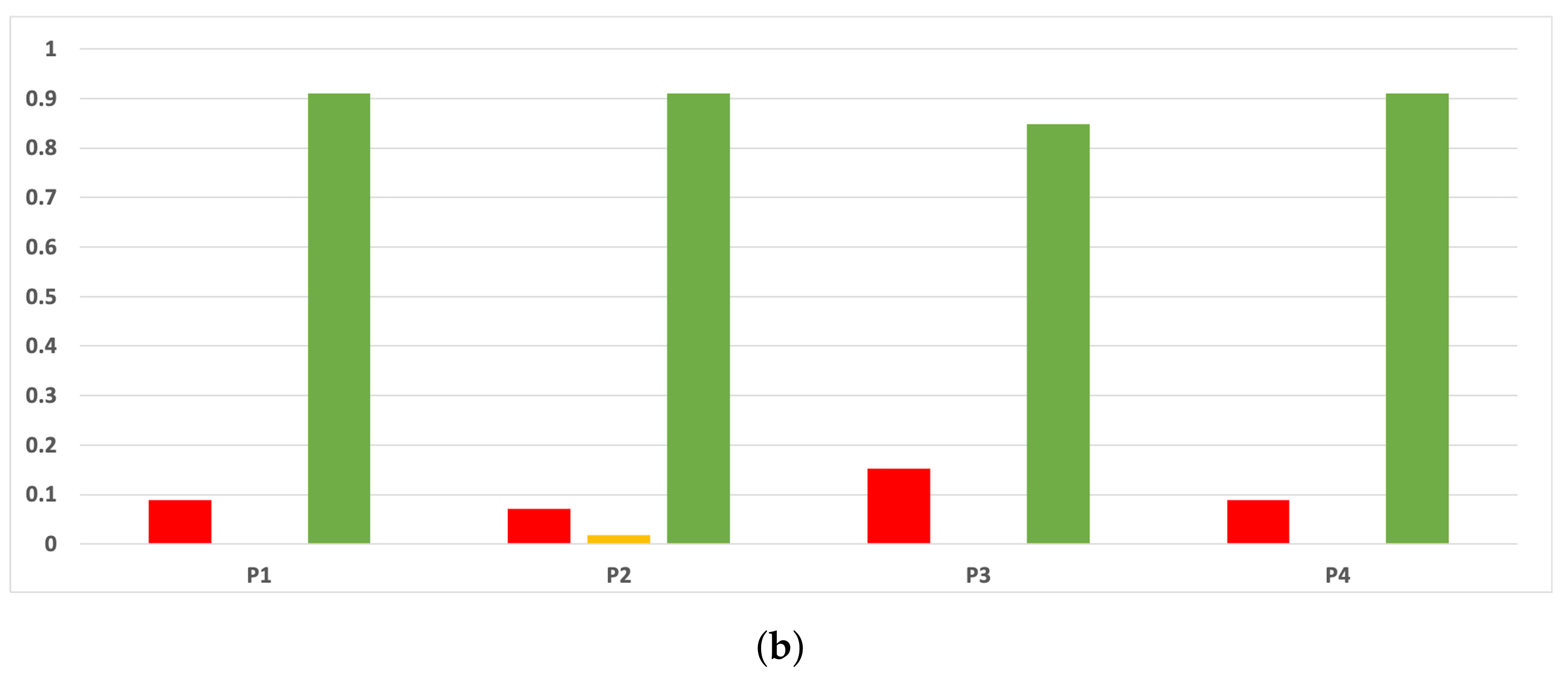
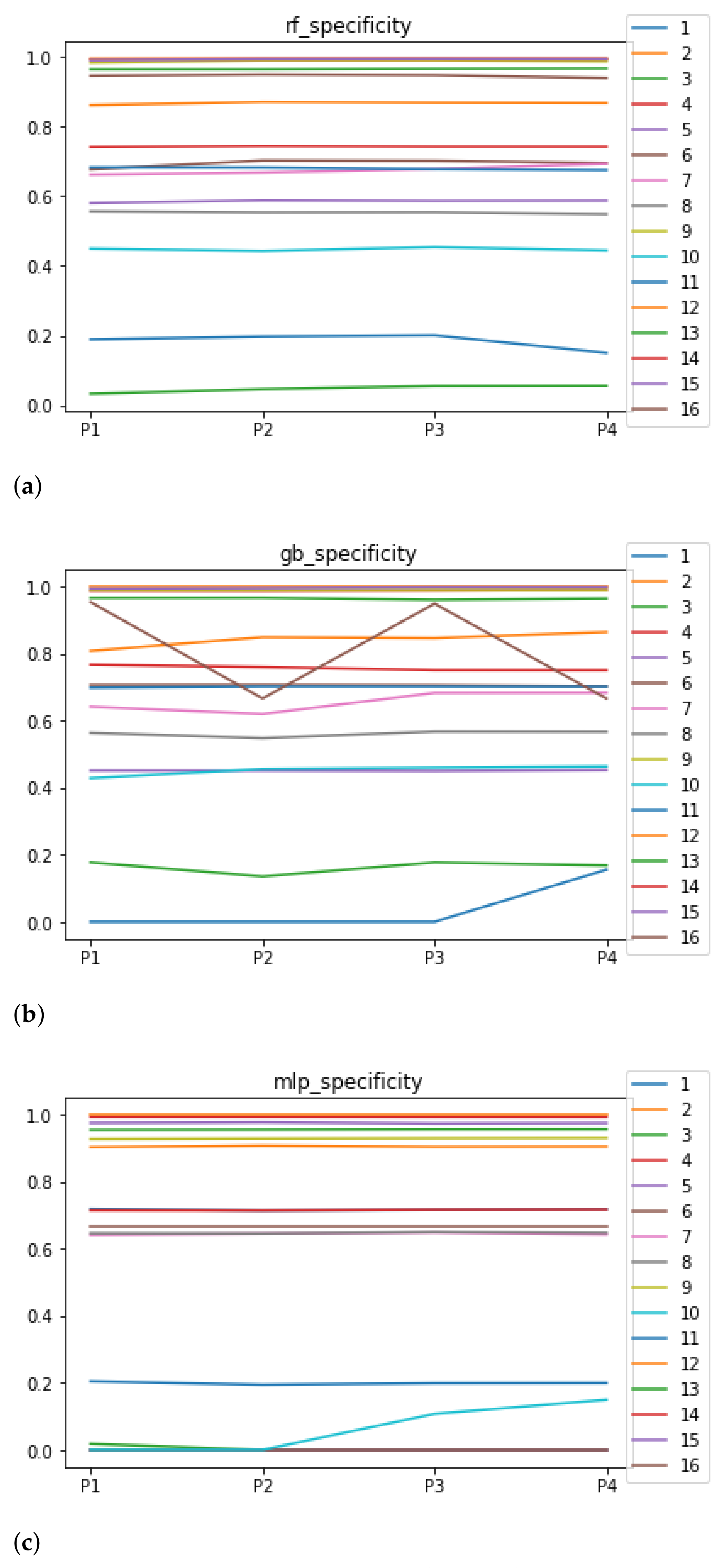
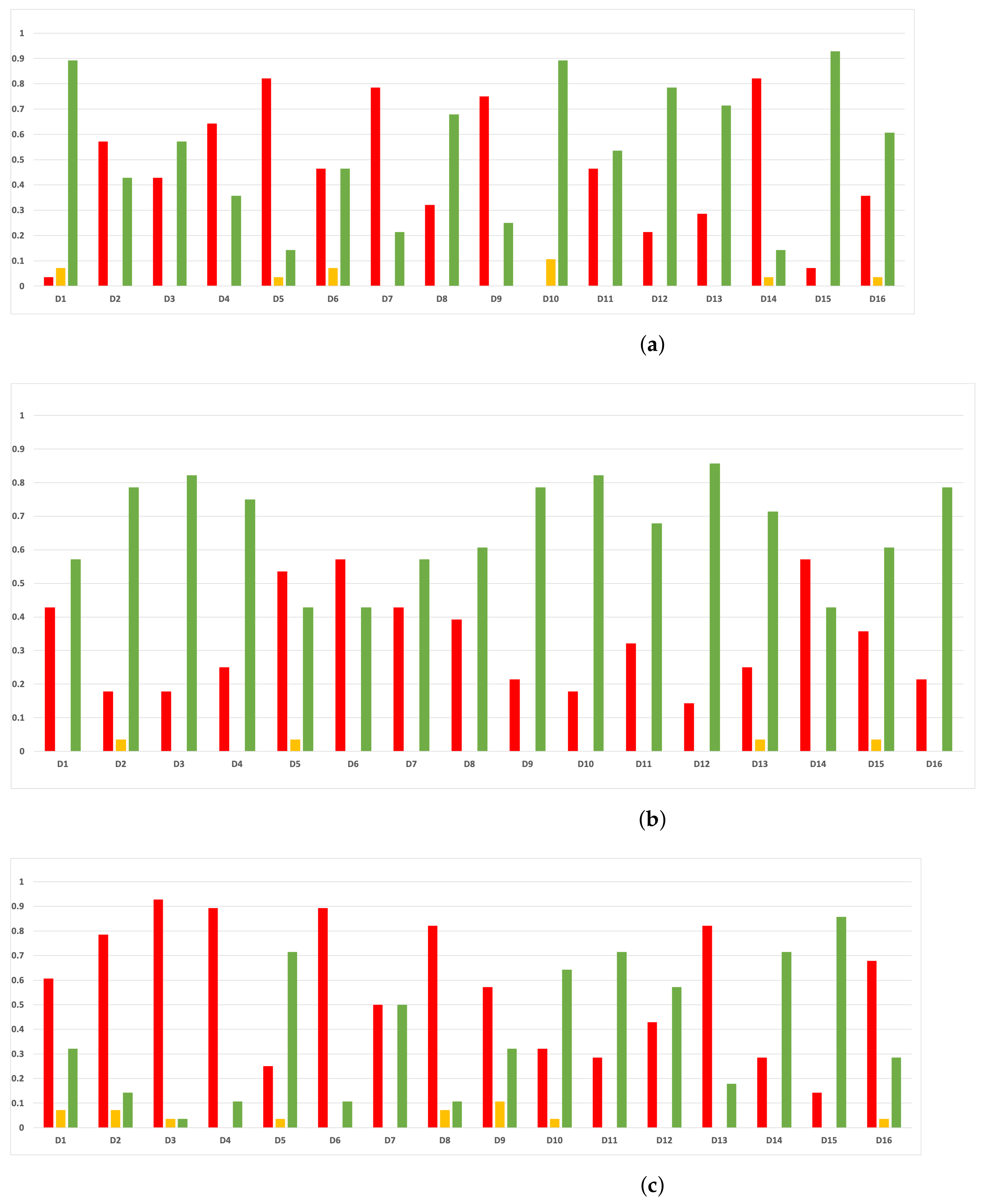
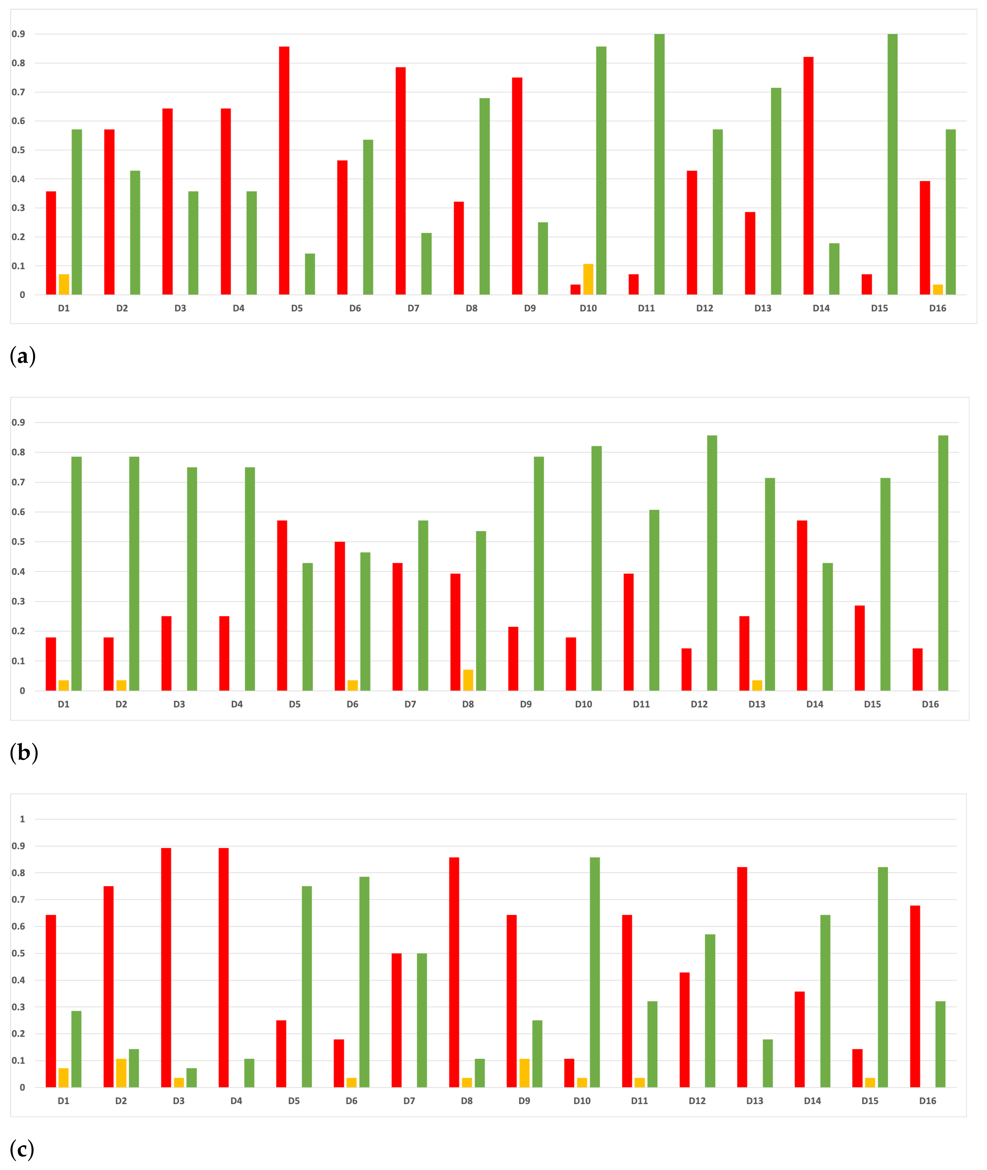
Figure 8.
Behavior RHOASo: specificity. The datasets are represented with a bar chart for each partition. (a) Specificity for RF. Axis X: the partition of the dataset. Axis Y: the obtained specificity. (b) Specificity for GB. Axis X: the partition of the dataset. Axis Y: the obtained specificity. (c) Specificity for MLP. Axis X: the partition of the dataset. Axis Y: the obtained specificity.
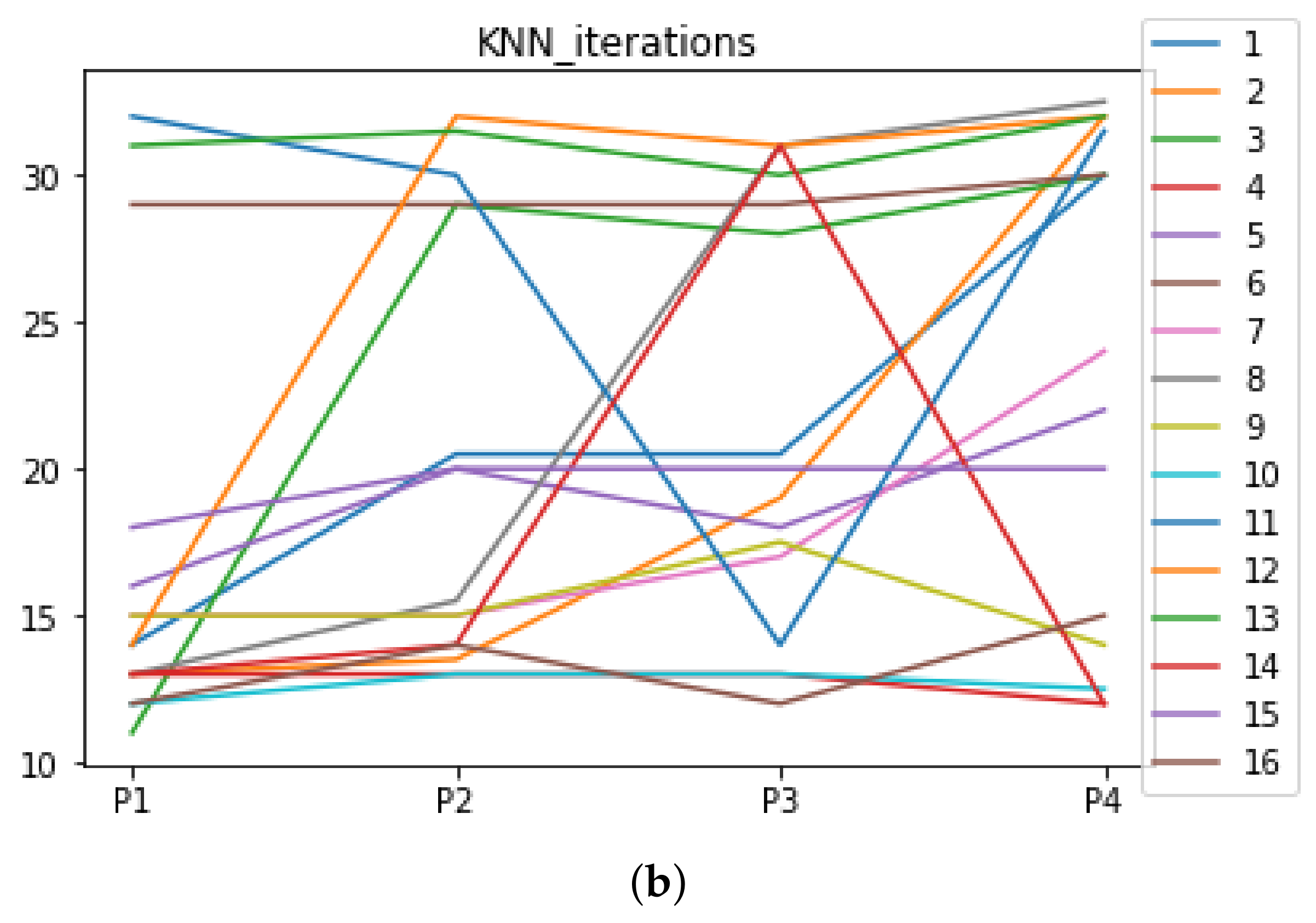
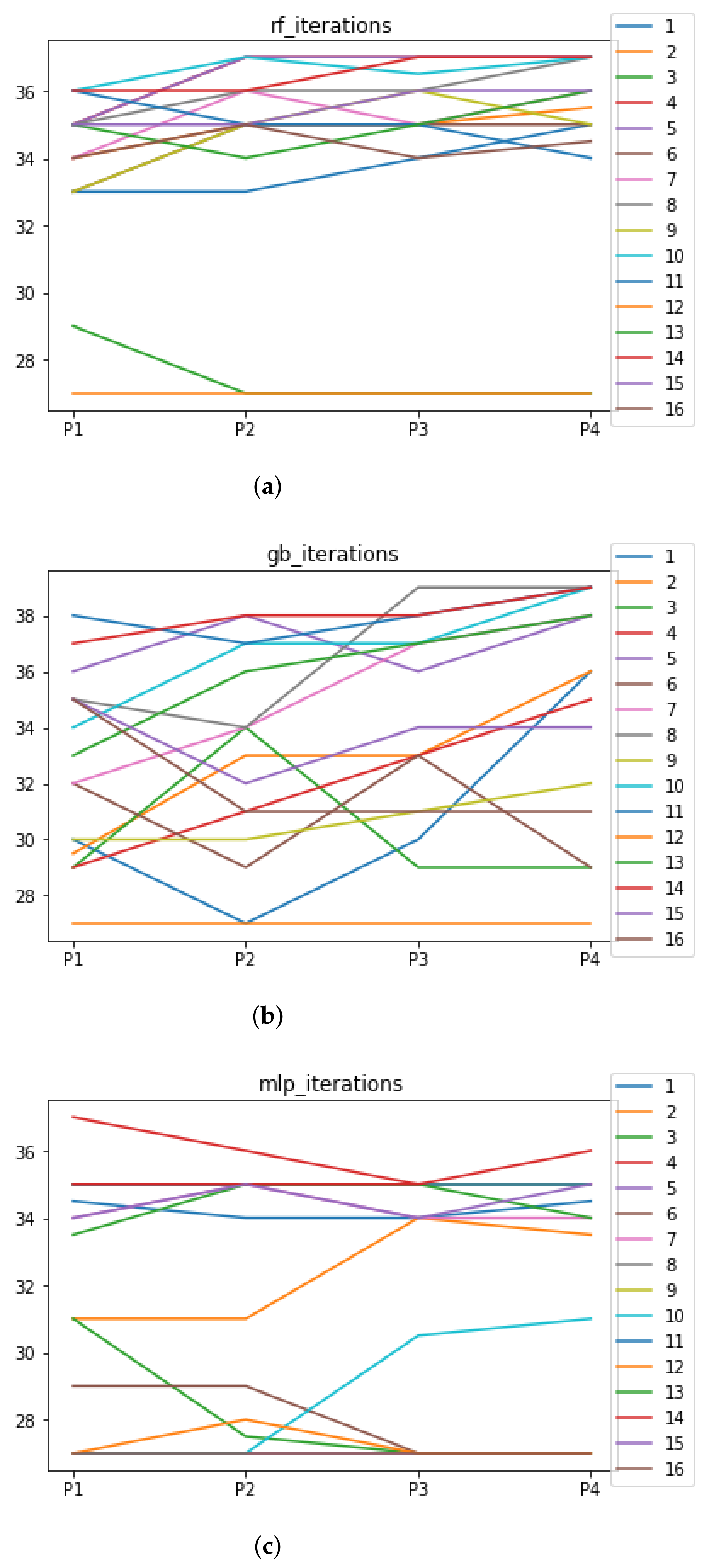
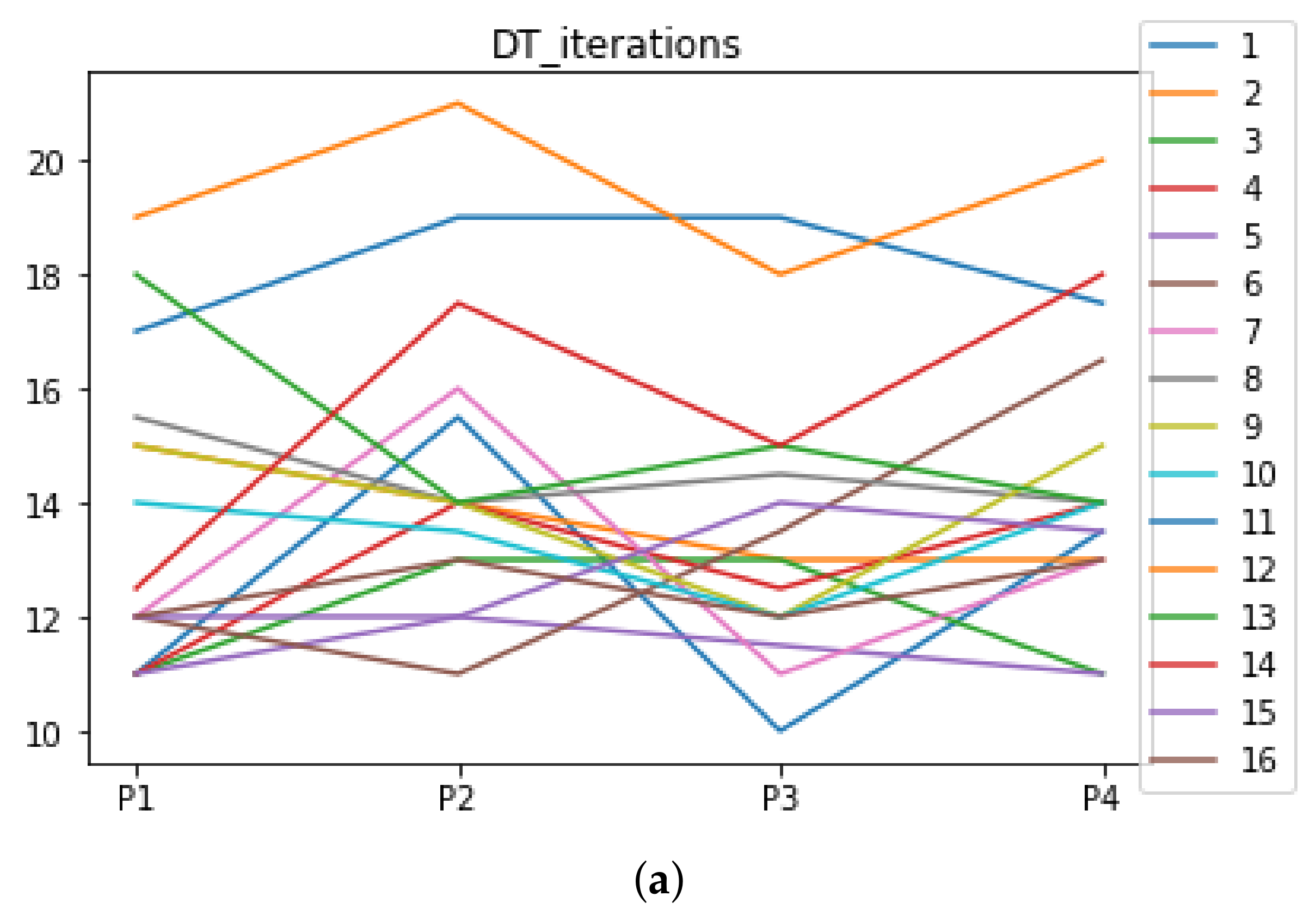
Figure 9.
Number of iterations per partition. Each line represents a dataset (medians). (a) Number of iterations RF. In axis X, the partition of the dataset. In axis Y, the number of the iterations that RHOASo has carried out. (b) Number of iterations GB. In axis X, the partition of the dataset. In axis Y, the number of the iterations that RHOASo has carried out. (c) Number of iterations MLP. In axis X, the partition of the dataset. In axis Y, the number of the iterations that RHOASo has carried out.
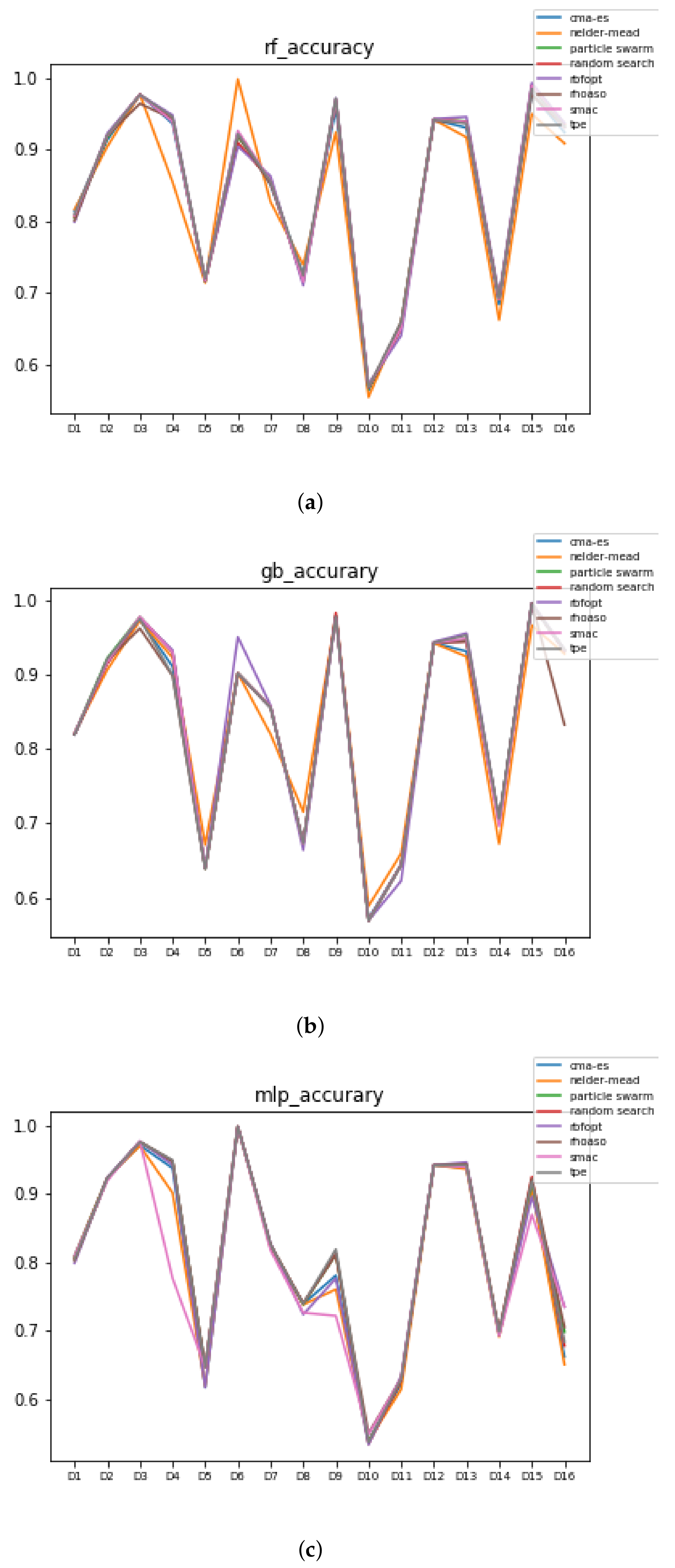
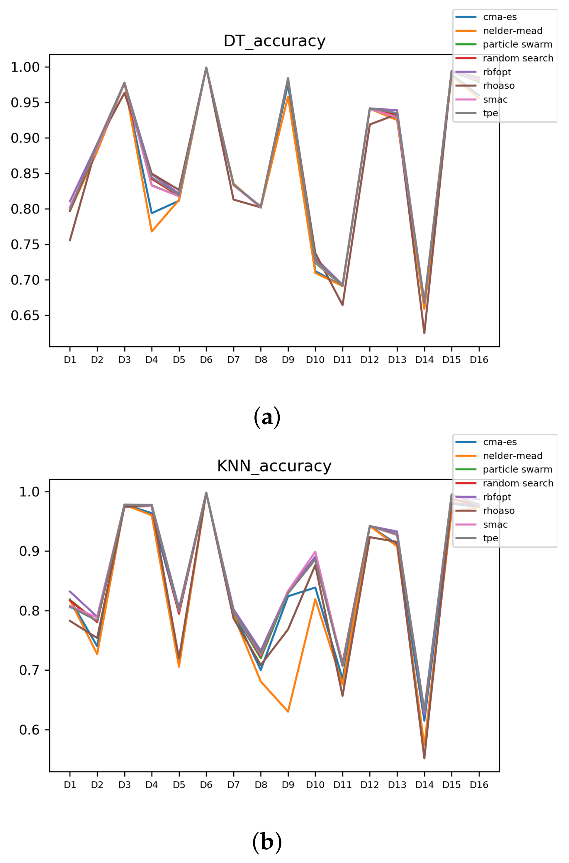
Figure 10.
Accuracy complexity. (a) Accuracy in RF. In axis X, the dataset. In axis Y, the accuracy obtained. Each line represents a HPO algorithm. (b) Accuracy in GB. In axis X, the dataset. In axis Y, the accuracy obtained. Each line represents a HPO algorithm. (c) Accuracy in MLP. In axis X, the dataset. In axis Y, the accuracy obtained. Each line represents a HPO algorithm.
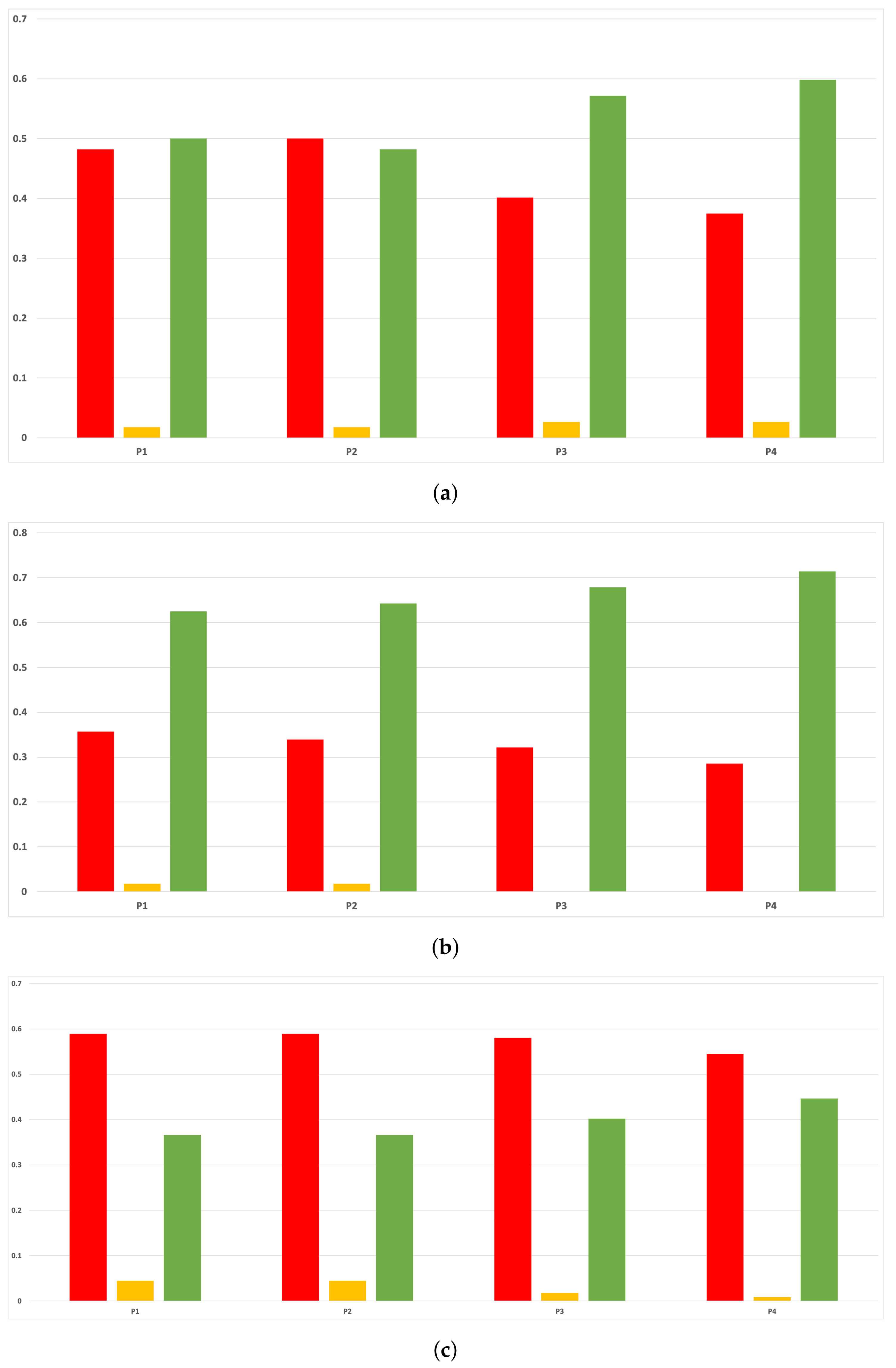
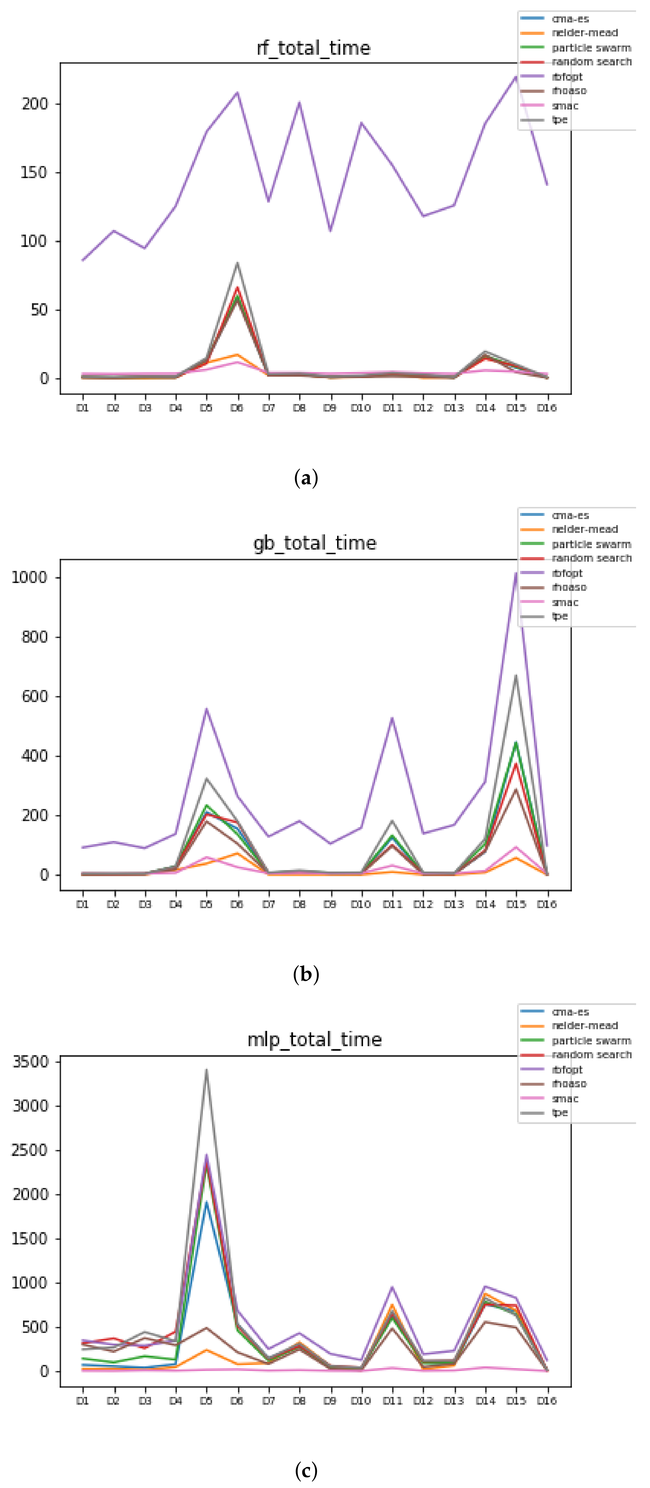
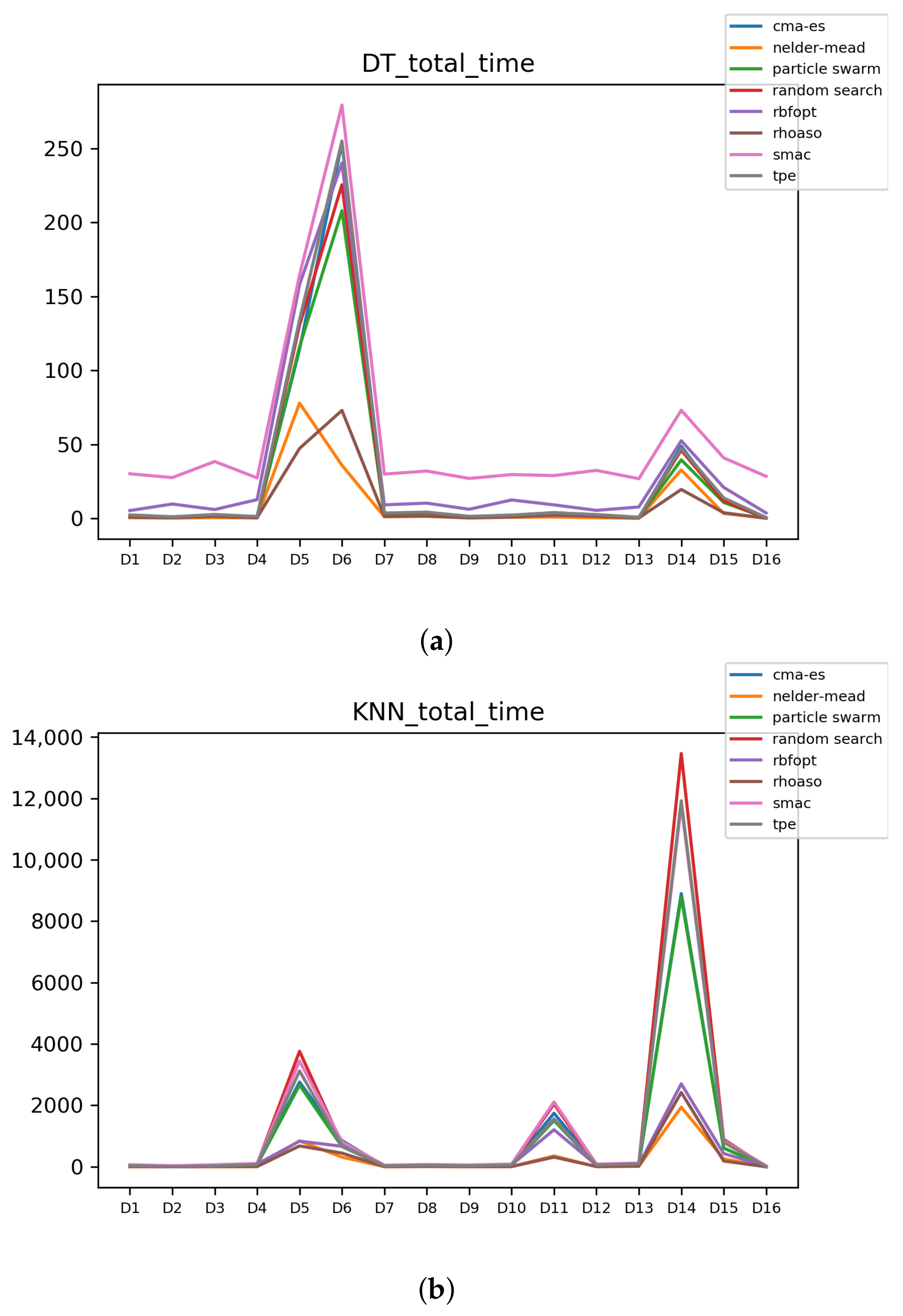
Figure 11.
Time complexity. (a) Time complexity in RF. In axis X, the dataset. In axis Y, the total time obtained measured in seconds. Each line represents a HPO algorithm. (b) Time complexity in GB. In axis X, the dataset. In axis Y, the total time obtained measured in seconds. Each line represents a HPO algorithm. (c) Time complexity in MLP. In axis X, the dataset. In axis Y, the total time obtained measured in seconds. Each line represents a HPO algorithm.
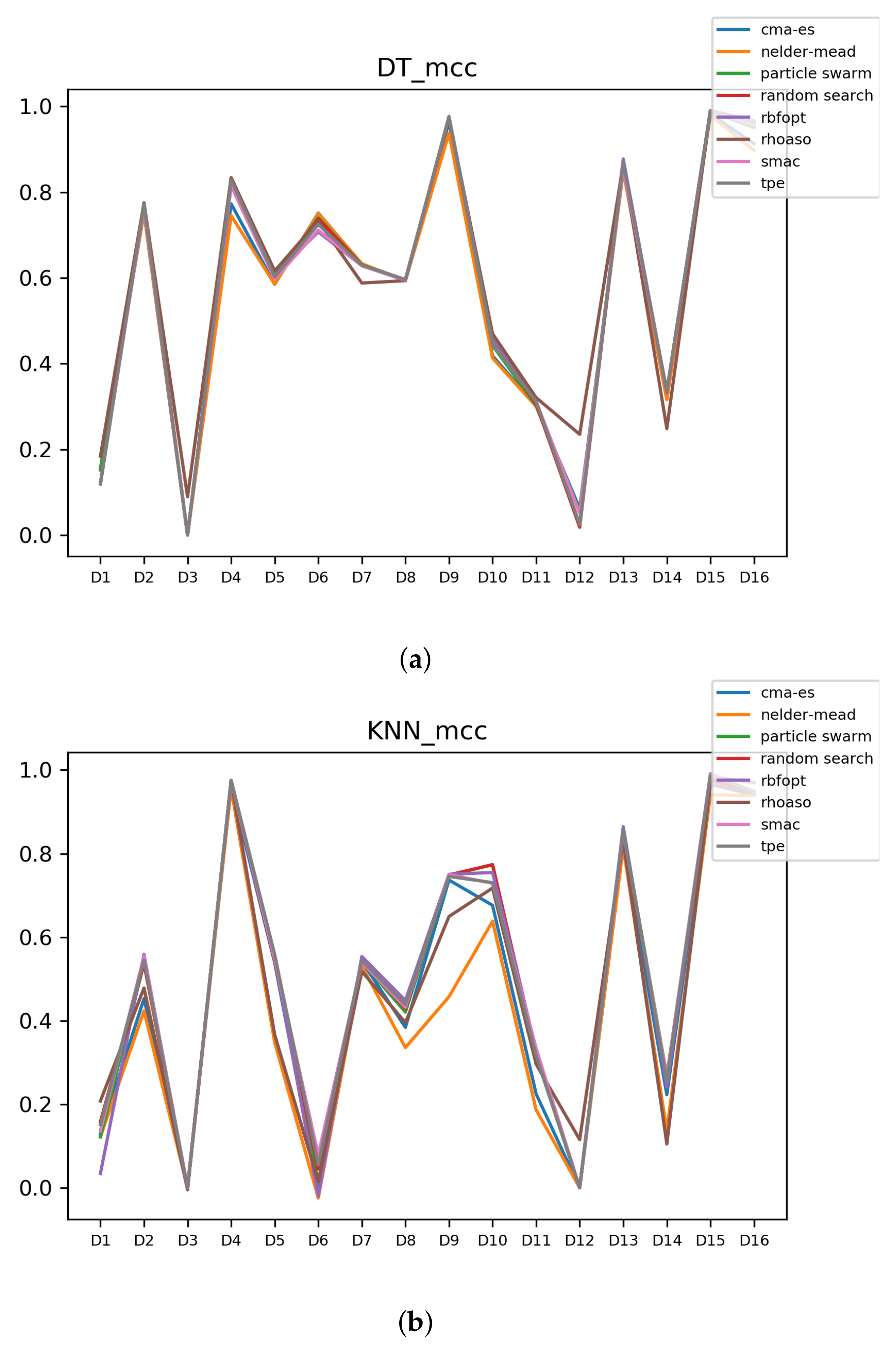
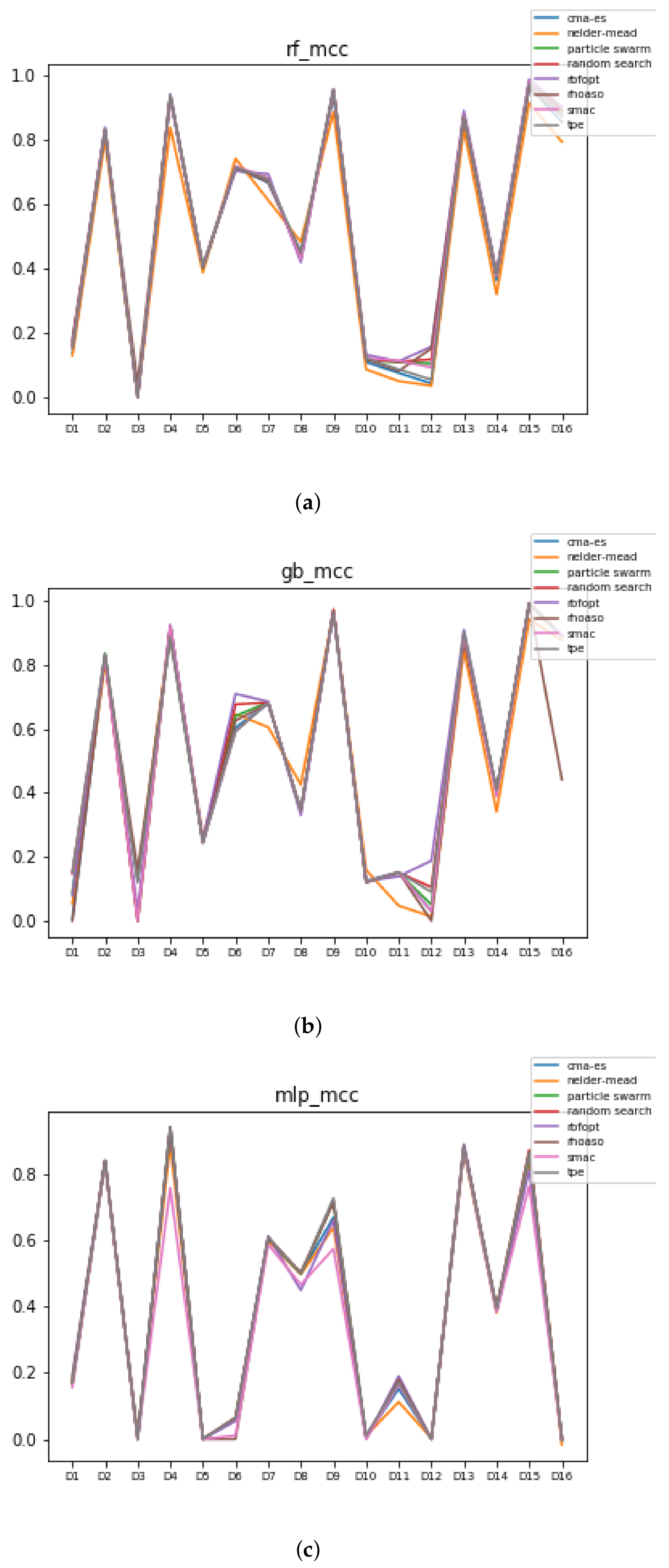
Figure 12.
MCC of all HPO algorithms. (a) MCC in RF. In axis X, the dataset. In axis Y, the MCC obtained. Each line represents a HPO algorithm. (b) MCC in GB. In axis X, the dataset. In axis Y, the MCC obtained. Each line represents a HPO algorithm. (c) MCC in MLP. In axis X, the dataset. In axis Y, the MCC obtained. Each line represents a HPO algorithm.
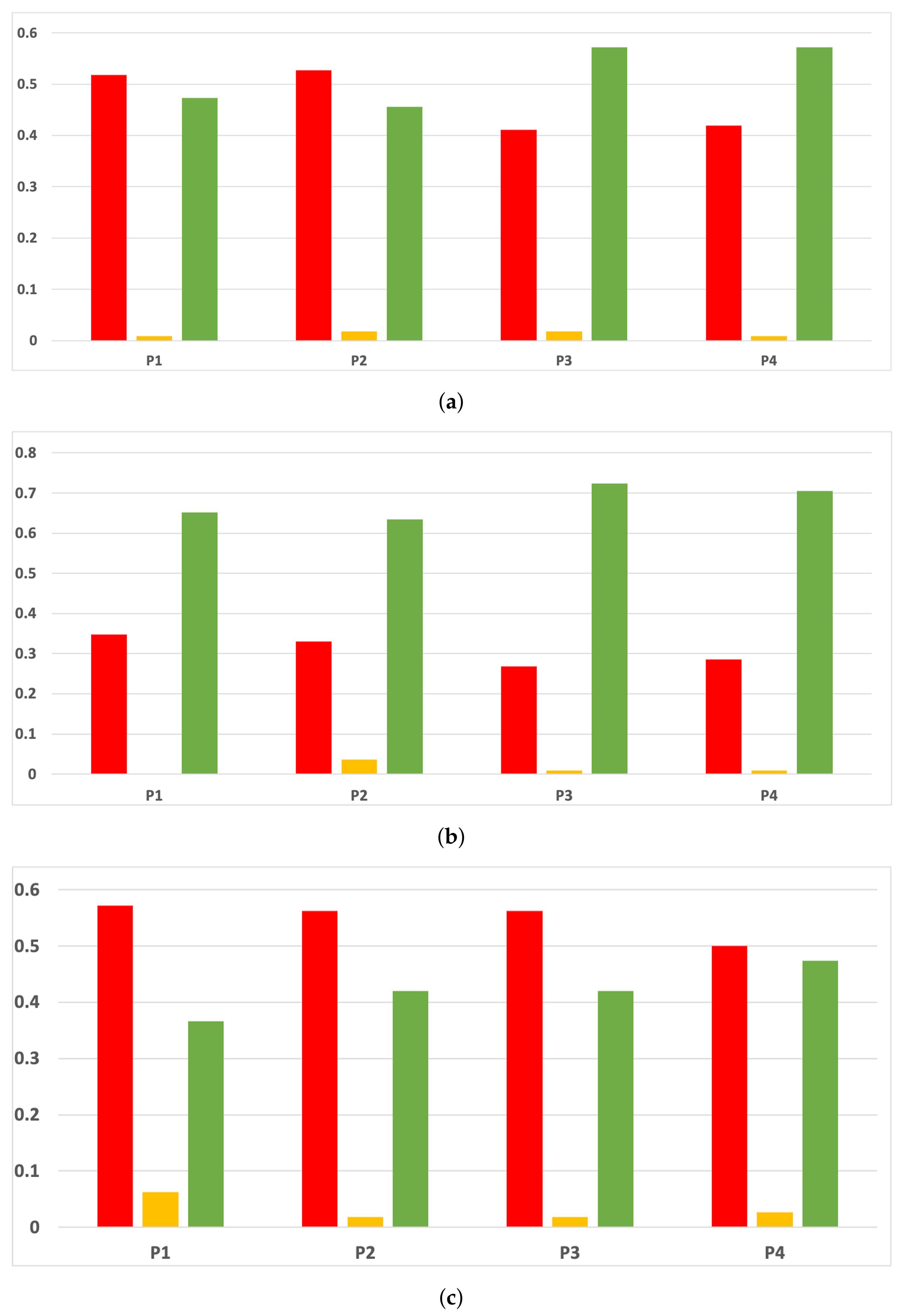
Figure 13.
Experiment 2: Accuracy complexity. (a) Accuracy in RF. In axis X, the dataset. In axis Y, the accuracy obtained. Each line represents a HPO algorithm. (b) Accuracy in GB. In axis X, the dataset. In axis Y, the accuracy obtained. Each line represents a HPO algorithm. (c) Accuracy in MLP. In axis X, the dataset. In axis Y, the accuracy obtained. Each line represents a HPO algorithm.
Figure 14.
Experiment 2: Time complexity. (a) Time complexity in RF. In axis X, the dataset. In axis Y, the total time obtained measured in seconds. Each line represents a HPO algorithm. (b) Time complexity in GB. In axis X, the dataset. In axis Y, the total time obtained measured in seconds. Each line represents a HPO algorithm. (c) Time complexity in MLP. In axis X, the dataset. In axis Y, the total time obtained measured in seconds. Each line represents a HPO algorithm.
Figure 15.
Experiment 2: MCC of all HPO algorithms. (a) MCC in RF. In axis X, the dataset. In axis Y, the MCC obtained. Each line represents a HPO algorithm. (b) MCC in GB. In axis X, the dataset. In axis Y, the MCC obtained. Each line represents a HPO algorithm. (c) MCC in MLP. In axis X, the dataset. In axis Y, the MCC obtained. Each line represents a HPO algorithm.
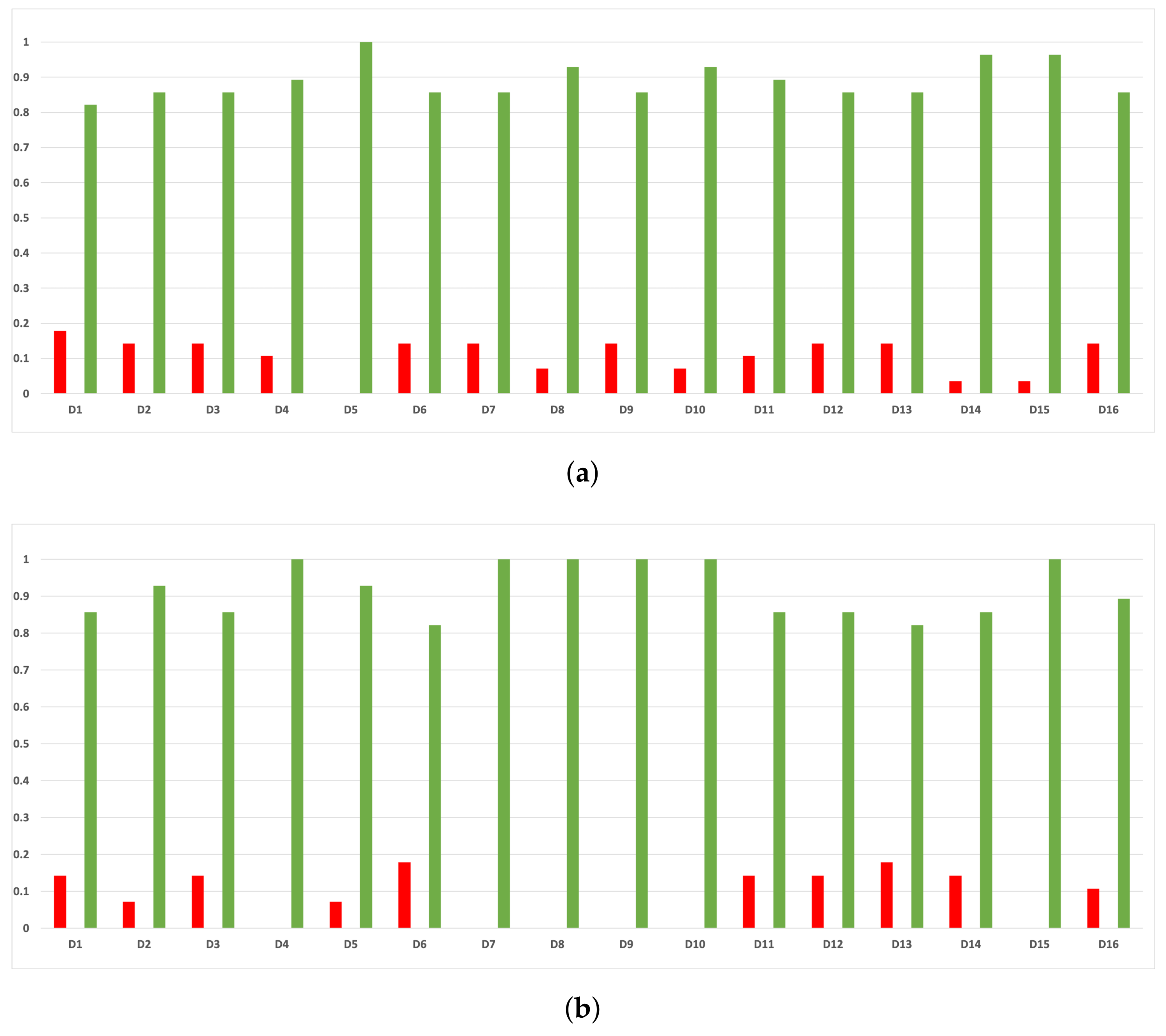
Figure 16.
Experiment 1: consistency per partition (accuracy and time complexity). (a) Rate of validity per partition in RF. In axis X, the partition of the dataset. In axis Y, the rate of RHOASo for each class of validity. (b) Rate of validity per partition in GB. In axis X, the partition of the dataset. In axis Y, the rate of RHOASo for each class of validity. (c) Rate of validity per partition in MLP. In axis X, the partition of the dataset. In axis Y, the rate of RHOASo for each class of validity.
Figure 17.
Experiment 1: consistency per dataset. Rate of validity with the accuracy and time complexity. (a) Rate of vx per dataset in RF. In axis X, the dataset. In axis Y, the rate of RHOASo for each class of validity. (b) Rate of validity per dataset in GB. In axis X, the dataset. In axis Y, the rate of RHOASo for each class of validity. (c) Rate of validity per dataset in MLP. In axis X, the dataset. In axis Y, the rate of RHOASo for each class of validity.
Figure 18.
Experiment 1: consistency per partition (MCC and time complexity). (a) Rate of validity per partition in RF. In axis X, the partition of the dataset. In axis Y, the rate of RHOASo for each class of validity. (b) Rate of validity per partition in GB. In axis X, the partition of the dataset. In axis Y, the rate of RHOASo for each class of validity. (c) Rate of validity per partition in MLP. In axis X, the partition of the dataset. In axis Y, the rate of RHOASo for each class of validity.
Figure 19.
Consistency per dataset: rate of validity with the MCC and time complexity. (a) Rate of validity per dataset in RF. In axis X, the dataset. In axis Y, the rate of RHOASo for each class of validity. (b) Rate of validity per dataset in GB. In axis X, the dataset. In axis Y, the rate of RHOASo for each class of validity. (c) Rate of validity per dataset in MLP. In axis X, the dataset. In axis Y, the rate of RHOASo for each class of validity.
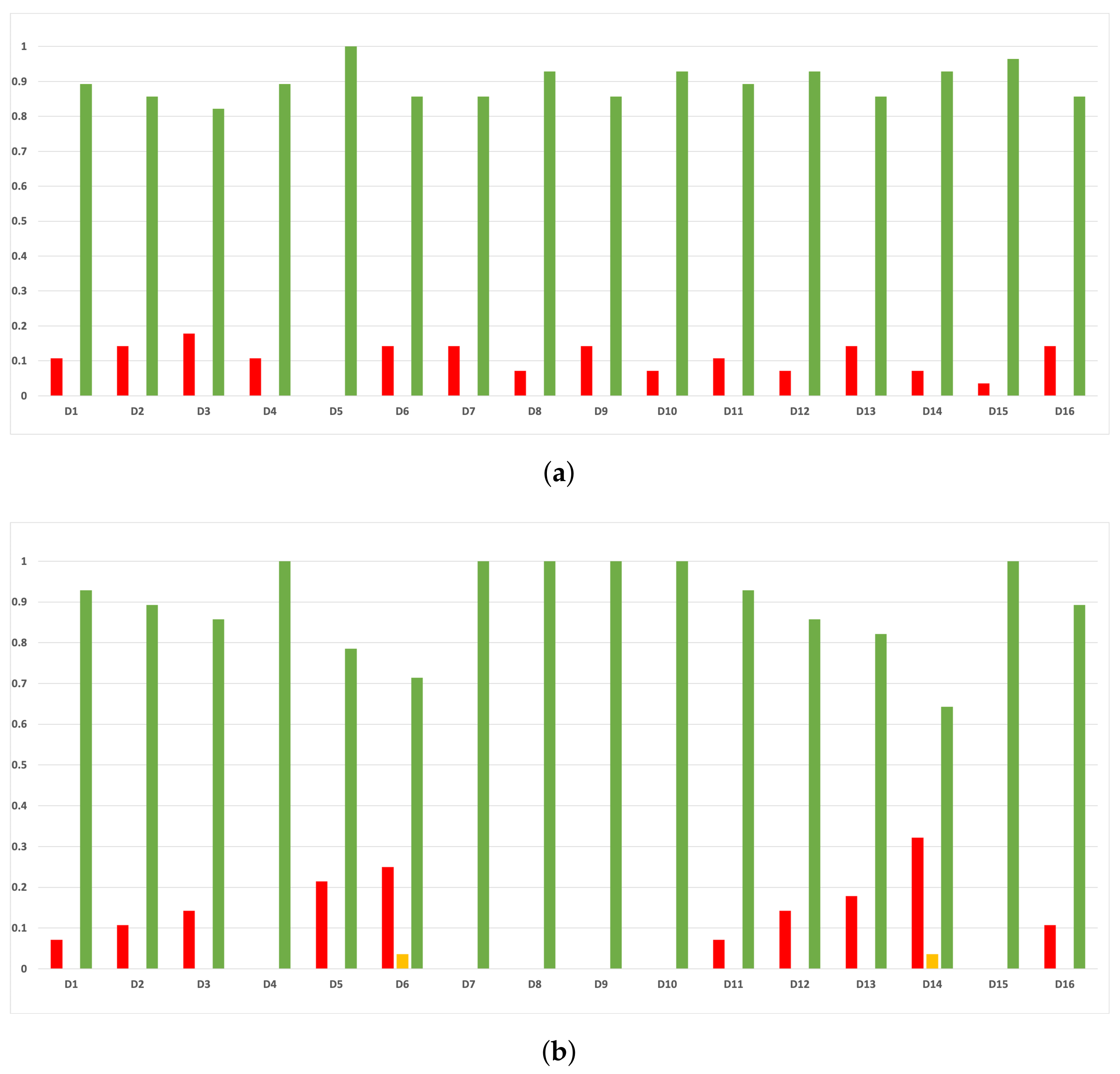
Figure 20.
Experiment 2: consistency per partition (accuracy and time complexity). (a) Rate of validity per partition in RF. In axis X, the partition of the dataset. In axis Y, the rate of RHOASo for each class of validity. (b) Rate of validity per partition in GB. In axis X, the partition of the dataset. In axis Y, the rate of RHOASo for each class of validity. (c) Rate of validity per partition in MLP. In axis X, the partition of the dataset. In axis Y, the rate of RHOASo for each class of validity.
Figure 21.
Experiment 2: consistency per dataset. Rate of validity with the accuracy and time complexity. (a) Rate of validity per dataset in RF. In axis X, the dataset. In axis Y, the rate of RHOASo for each class of validity. (b) Rate of validity per dataset in GB. In axis X, the dataset. In axis Y, the rate of RHOASo for each class of validity. (c) Rate of validity per dataset in MLP. In axis X, the dataset. In axis Y, the rate of RHOASo for each class of validity.
Figure 22.
Experiment 2: consistency per partition (MCC and time complexity). (a) Rate of validity per partition in RF. In axis X, the partition of the dataset. In axis Y, the rate of RHOASo for each class of validity. (b) Rate of validity per partition in GB. In axis X, the partition of the dataset. In axis Y, the rate of RHOASo for each class of validity. (c) Rate of validity per partition in MLP. In axis X, the partition of the dataset. In axis Y, the rate of RHOASo for each class of validity.
Figure 23.
Experiment 2: consistency per dataset. Rate of validity with the MCC and time complexity. (a) Rate of validity per dataset in RF. In axis X, the dataset. In axis Y, the rate of RHOASo for each class of validity. (b) Rate of validity per dataset in GB. In axis X, the dataset. In axis Y, the rate of RHOASo for each class of validity. (c) Rate of validity per dataset in MLP. In axis X, the dataset. In axis Y, the rate of RHOASo for each class of validity.
Table 1.
Open research challenge in HPO. Content extracted from [
3].
Table 1.
Open research challenge in HPO. Content extracted from [
3].
| Research Challenge | Description |
|---|
| HPO vs. CASH tools | Research conducted to specialized tools and algorithms for HPO or to CASH
(Combined algorithm selection and hyper-parameter optimization) problem |
| Monitoring HPO | Tools that let the user follow the progress in an interactive way |
| Less computational costs | HPO remains computationally extremely expensive for certain tasks |
| Overtuning HPO | Control resampling in an efficient way |
| Closed black-box | The user can not take decisions about the optimization process and cannot analyze the HPO procedure. |
| Not supervised learning | Developing HPO algorithms for more types of machine
learning models, not only for supervised ones. |
| Users do not make use of advanced HPO approaches | Potential users have a poor understanding of HPO methods.
Missing guidance makes difficult the choice and configuration of of HPO methods |
| Finishing an HPO method | There are several ways to configure the end of an HPO
method, not all of them are easily configurable. |
Table 2.
Hyper-parameters of the HPO algorithms considered in this work.
Table 2.
Hyper-parameters of the HPO algorithms considered in this work.
| Name | Hyper-Parameters | Library |
|---|
| Particle Swarm | 6 | [21] |
| Tree Parzen Estimators | 2 | [25] |
| CMA-ES | 3 | [26] |
| Nelder–Mead | 2 | [26] |
| Random Search | 1 | [26] |
| SMAC | 30 | [27] |
| RBFOpt | 46 | [28] |
Table 3.
ML algorithms together with hyper-parameters we have considered.
Table 3.
ML algorithms together with hyper-parameters we have considered.
| Name | Hyper-Parameter 1 | Hyper-Parameter 2 |
|---|
| RF | Num. Trees | Max. Depth |
| GB | Num. Trees | Max. Depth |
| MLP (2 hidden layers) | Num. Neurons Layer 1 | Num. Neurons Layer 2 |
Table 4.
HPO algorithms used. Colors explanation: Bayesian methods in blue, decision-theoretic techniques in pink, evolutionary algorithms in brown, and other optimization algorithms in green.
Table 4.
HPO algorithms used. Colors explanation: Bayesian methods in blue, decision-theoretic techniques in pink, evolutionary algorithms in brown, and other optimization algorithms in green.
| Name | Reference | Python
Version | Automatic
Early Stop | Library |
|---|
| Particle Swarm | [20,35] | 2.7 y 3 | X | [21] |
| Tree Parzen Estimators | [10] | 2.7, 3 | X | [25] |
| CMA-ES | [17] | 2.7, 3 | X | [26] |
| Nelder–Mead | [18] | 2.7, 3 | √ | [26] |
| Random Search | [15] | 2.7, 3 | X | [26] |
| SMAC | [9] | 3 | X | [27] |
| RBFOpt | [11,36] | 2.7, 3 | X | [28] |
Table 5.
Descriptions of datasets.
Table 5.
Descriptions of datasets.
| Dataset = | Topic | Classes | Majority Class
Proportion | Features | Instances = | | | | Reference |
|---|
| First order proving | 2 | 0.82 | 51 | 4589 | 382 | 764 | 2294 | [37] |
| Spambase | 2 | 0.6 | 57 | 4601 | 383 | 766 | 2300 | [38] |
| Polish companies | 2 | 0.978 | 64 | 4885 | 407 | 814 | 2442 | [39] |
| | Bankruptcy | | | | | | | | |
| Opto digits | 10 | 0.1 | 64 | 5620 | 468 | 936 | 2810 | [40] |
| Grammatical | 2 | 0.64 | 300 | 27,936 | 2328 | 4656 | 13,968 | [41] |
| | Facial Expressions | | | | | | | | |
| Credit card | 2 | 0.99 | 30 | 284,807 | 23,733 | 47,467 | 142,403 | [42] |
| | Fraud Detection | | | | | | | | |
| Magic Telescope | 2 | 0.64 | 10 | 19,020 | 1585 | 3170 | 9519 | [43] |
| Electricity | 2 | 0.57 | 8 | 45,312 | 3776 | 7552 | 22,656 | [44,45] |
| Wall Robot | 4 | 0.4 | 24 | 5456 | 454 | 909 | 2728 | [46] |
| Eye | 2 | 0.55 | 14 | 14,980 | 1248 | 2496 | 7490 | [47] |
| Connect 4 | 3 | 0.65 | 43 | 67,557 | 5629 | 11,259 | 33,778 | [48] |
| Amazon | 2 | 0.94 | 9 | 32,769 | 2730 | 5461 | 16,384 | [49] |
| Phishing websites | 2 | 0.55 | 30 | 11,055 | 921 | 1842 | 5527 | [50] |
| Higgs | 2 | 0.52 | 28 | 98,049 | 8170 | 16,341 | 49,025 | [51] |
| NSL-KDD | 6 | 0.51 | 42 | 148,517 | 12,376 | 24,752 | 74,258 | [52,53] |
| Robots in RTLS | 3 | 0.73 | 12 | 6422 | 535 | 1070 | 3211 | [54] |
Table 6.
Conditions of validity. The symbols =, >, < denote statistically meaningful equality and difference, and Me denotes the median.
Table 6.
Conditions of validity. The symbols =, >, < denote statistically meaningful equality and difference, and Me denotes the median.
| Validity | Pj | | | |
|---|
| | | | |
|
| | | |
|
| | | |
|
| | | |
Table 7.
Medians of response variables for RHOASo in Experiment 2.
Table 7.
Medians of response variables for RHOASo in Experiment 2.
| Dataset | Accuracy | MCC | Time Complexity | Sensitivity | Specificity | Iterations |
|---|
| D1
| RF | 0.8024 | 0.1776 | 0.904 | 0.9419 | 0.1743 | 32.0 |
| GB | 0.8194 | 0.0002 | 1.2169 | 0.9999 | 0.0 | 30.5 |
| MLP | 0.8018 | 0.1811 | 256.0706 | 0.9367 | 0.1971 | 35.0 |
| D2
| RF | 0.923 | 0.8394 | 0.7208 | 0.9563 | 0.8732 | 37 |
| GB | 0.9108 | 0.8141 | 1.0615 | 0.9675 | 0.8274 | 28.5 |
| MLP | 0.9244 | 0.8432 | 237.3997 | 0.9362 | 0.9079 | 32.5 |
| D3
| RF | 0.9632 | 0.0496 | 0.9074 | 0.9835 | 0.0573 | 27.0 |
| GB | 0.9681 | 0.1249 | 1.29 | 0.9866 | 0.1127 | 29.0 |
| MLP | 0.9771 | 0.0 | 280.6122 | 0.999 | 0.0 | 27.0 |
| D4
| RF | 0.9499 | 0.9445 | 0.8897 | 0.95 | 0.9944 | 37.0 |
| GB | 0.8994 | 0.8886 | 14.3729 | 0.8994 | 0.9888 | 33.0 |
| MLP | 0.934 | 0.9269 | 339.9584 | 0.934 | 0.9927 | 34.5 |
| D5
| RF | 0.7175 | 0.4067 | 16.6164 | 0.7885 | 0.589 | 37.0 |
| GB | 0.6384 | 0.2443 | 189.5368 | 0.7401 | 0.4527 | 38.0 |
| MLP | 0.6464 | 0.0 | 321.7485 | 1.0 | 0 | 27.0 |
| D6
| RF | 0.9876 | 0.7332 | 35.5843 | 0.9916 | 0.6794 | 33.0 |
| GB | 0.9009 | 0.6211 | 127.1753 | 0.9013 | 0.6999 | 33.0 |
| MLP | 0.9922 | 0.0028 | 218.3069 | 1.0 | 0.0036 | 27.0 |
| D7
| RF | 0.8588 | 0.6845 | 2.4416 | 0.9483 | 0.6965 | 35.0 |
| GB | 0.8609 | 0.6916 | 5.1165 | 0.9629 | 0.673 | 37.0 |
| MLP | 0.8266 | 0.6106 | 109.3366 | 0.9256 | 0.6444 | 33.5 |
| D8
| RF | 0.7325 | 0.4688 | 2.4364 | 0.8881 | 0.5518 | 34.5 |
| GB | 0.6726 | 0.3437 | 9.2316 | 0.7504 | 0.567 | 38.0 |
| MLP | 0.7374 | 0.4963 | 225.6947 | 0.8138 | 0.6372 | 31.0 |
| D9
| RF | 0.9756 | 0.9635 | 1.1602 | 0.9549 | 0.9908 | 36.0 |
| GB | 0.9775 | 0.9664 | 3.9133 | 0.9508 | 0.9907 | 32.0 |
| MLP | 0.8014 | 0.7016 | 48.2327 | 0.765 | 0.9251 | 35.0 |
| D10
| RF | 0.5654 | 0.1156 | 1.2617 | 0.6625 | 0.445 | 37.0 |
| GB | 0.5703 | 0.1244 | 3.665 | 0.6664 | 0.4559 | 37.5 |
| MLP | 0.5457 | 0.0021 | 10.986 | 0.9297 | 0.0709 | 27.0 |
| D11
| RF | 0.6583 | 0.0276 | 1.3408 | 0.3358 | 0.6683 | 33.0 |
| GB | 0.6434 | 0.1519 | 77.7497 | 0.381 | 0.7023 | 38.0 |
| MLP | 0.6309 | 0.1779 | 534.4388 | 0.4034 | 0.7164 | 34.0 |
| D12
| RF | 0.9406 | 0.1435 | 1.1293 | 0.068 | 0.9938 | 29.0 |
| GB | 0.9421 | 0.0 | 0.9947 | 0.0 | 1.0 | 27.0 |
| MLP | 0.942 | 0.0 | 50.6516 | 0.0 | 0.9999 | 27.0 |
| D13
| RF | 0.9436 | 0.886 | 0.6895 | 0.9124 | 0.9682 | 37.0 |
| GB | 0.9474 | 0.8936 | 1.303 | 0.9273 | 0.9649 | 34.0 |
| MLP | 0.9427 | 0.8841 | 94.5033 | 0.9245 | 0.957 | 34.5 |
| D14
| RF | 0.6897 | 0.3766 | 20.5842 | 0.6307 | 0.7431 | 38.0 |
| GB | 0.7068 | 0.4104 | 81.4707 | 0.6568 | 0.7517 | 38.0 |
| MLP | 0.7003 | 0.3993 | 515.4725 | 0.6811 | 0.7177 | 37.0 |
| D15
| RF | 0.9782 | 0.9608 | 4.5483 | 0.6555 | 0.9933 | 33.5 |
| GB | 0.9919 | 0.9885 | 305.4672 | 0.9417 | 0.9987 | 35.5 |
| MLP | 0.9217 | 0.8595 | 474.1431 | 0.5171 | 0.9739 | 34.0 |
| D16
| RF | 0.9312 | 0.8643 | 0.5872 | 0.8498 | 0.9385 | 35.0 |
| GB | 0.8687 | 0.6586 | 0.9878 | 0.7524 | 0.8705 | 30.0 |
| MLP | 0.7348 | 0.0 | 11.8172 | 0.3333 | 0.6667 | 27.0 |
Table 8.
Rate of validity of RHOASo vs. HPO across all (% with accuracy and time complexity).
Table 8.
Rate of validity of RHOASo vs. HPO across all (% with accuracy and time complexity).
| Validity | RF | GB | MLP | Average |
|---|
| | | | |
| | | | |
| | | | |
| | | | |
Table 9.
Rate of validity of RHOASo vs. HPO across all (% with accuracy and time complexity).
Table 9.
Rate of validity of RHOASo vs. HPO across all (% with accuracy and time complexity).
| Validity | RF | GB | MLP | Average |
|---|
| | | | |
| | | | |
| | | | |
Table 10.
Rate of validity of RHOASo vs. HPO across all (% with MCC and time complexity).
Table 10.
Rate of validity of RHOASo vs. HPO across all (% with MCC and time complexity).
| Validity | RF | GB | MLP | Average |
|---|
| | | | |
| | | | |
| | | | |
Table 11.
Experiment 2: Rate of validity of RHOASo vs. HPO across all (% with accuracy and time complexity).
Table 11.
Experiment 2: Rate of validity of RHOASo vs. HPO across all (% with accuracy and time complexity).
| Validity | RF | GB | MLP | Average |
|---|
| | | | |
| | | | |
| | | | |
Table 12.
Experiment 2: rate of validity of RHOASo Vs HPO across all (% with MCC and time complexity).
Table 12.
Experiment 2: rate of validity of RHOASo Vs HPO across all (% with MCC and time complexity).
| Validity | RF | GB | MLP | Average |
|---|
| | | | |
| | | | |
| | | | |


