Quasi-Interpolation in a Space of C² Sextic Splines over Powell–Sabin Triangulations

Abstract

In this work, we study quasi-interpolation in a space of sextic splines defined over Powell–Sabin triangulations. These spline functions are of class $C^2$ on the whole domain but fourth-order regularity is required at vertices and $C^3$ regularity is imposed across the edges of the refined triangulation and also at the interior point chosen to define the refinement. An algorithm is proposed to define the Powell–Sabin triangles with a small area and diameter needed to construct a normalized basis. Quasi-interpolation operators which reproduce sextic polynomials are constructed after deriving Marsden’s identity from a more explicit version of the control polynomials introduced some years ago in the literature. Finally, some tests show the good performance of these operators.

1. Introduction

Spline functions over triangulations have been, and are, the object of intense research for their role in the Approximation Theory and for dealing with a wide variety of problems of practical interest, among which the approximation of scattered data and the numerical solution of partial differential equations occupy a prominent place.

It is well known that the requirement of a regularity $C^m$ of a spline on a given triangulation implies that the degree must be greater than or equal to $4m+1$ [1]. As in practice, it is essential to use splines of the lowest degree for a given class, different finite elements obtained by subdiving every triangle have been introduced and analyzed in the literature, among them the Clough–Tocher (CT-) and Powell–Sabin (PS-) refinements (see [2] and [3], respectively).

The PS-refinement was proposed in [3] for contour plotting. A first subdivision into six triangles is achieved by selecting an inner point in every triangle and connecting it with similar points in the adjacent triangles as well as with the three vertices. The inner point of a boundary triangle is joined to a point over a boundary edge when no adjacent triangle is available. From this PS6-split, a PS12-split is easily derived by joining in every triangle the three points lying on the edges of the triangle that the previous construction produces [4]. Furthermore, in this case, PS-splines of higher degree and smoothness have been constructed [5].

Since their introduction, $C^1$ quadratic splines on Powell–Sabin (PS-) triangulations found several useful applications in interpolation and linear least squares fitting. Especially, we mention the papers [6,7,8,9] treating numerical solution of PDEs, and the references [10] concerned with interpolation and least squares subject to one- or two-sided restrictions. The construction of quasi-interpolation operators with optimal orders is treated in [11,12,13,14,15,16,17]. Gaussian quadrature rules are also treated using $C^1$ quadratic Powell–Sabin (PS-) splines [18].

The application of splines in various fields requires efficient algorithms for constructing locally supported bases for the spline spaces. The B-spline representation of bivariate $C^1$ quadratic splines achieved by Dierckx [19] was essential in the development of spline spaces on PS partitions and applications. The method proposed by P. Dierckx is completely geometrical, it is reduced to finding a set of PS2 triangles that must contain a number of specified points. Linear and quadratic programming problems are the standard methods proposed by many authors in the literature [19,20]. The main idea of both methods is to minimize the area of a triangle without imposing any condition concerning the diameter of the sought triangles. Moreover, the quadratic problem only provides local maxima. In order to avoid these limitations, we present an algorithm that aims to produce PS6 triangles with a smaller area and diameter, and compare it with the one proposed in [21].

The study of spline function spaces on Powell–Sabin partitions obtained by a refinement into six sub-triangles, has attracted a great interest in the scientific community since its introduction. The cubic case was considered in [20,22]. Spaces of quintic splines were analyzed in [23] and more recently in [24], among others. In [25] and [26], normalized bases for PS-splines of degree $3r-1$ are defined and super-splines of arbitrary degree are given, respectively.

Quasi-interpolation over Powell–Sabin triangulations for specific spaces have been also studied in depth [11,12,13,14,15,16,17,24], as well as for a family of spaces [27]. The construction of such operators is based on establishing a Marsden’s identity. It is a powerful tool that allows to write the monomials in terms of the corresponding B-spline-like functions (B-splines for short). In this view, we establish a general Marsden’s identity in the subspace of sextic splines from an easy approach based on a version of the control polynomials different from the one used in [25].

In this paper, we revise a subspace of $C^2$ sextic PS6 splines obtained by imposing additional smoothness requirements at the interior points of the triangulation chosen to construct the sub-triangulation and also across some edges of the refined triangulation. This subspace of splines was studied in [26], where it is shown that every spline is uniquely determined by its values at the vertices of the initial triangulation and the interior points and those of its partial derivatives up to the fourth order at the vertices.

The paper is organized as follows: In Section 2, we recall some general concepts of polynomials on triangles and recall the notion of control polynomials. In Section 3, we recall some results concerning the space of sextic PS6 splines as well as the Hermite interpolation problems needed to obtain the B-splines forming a normalized basis, and provide explicit expressions for the Bernstein–Bézier coefficients of the B-splines in order to provide a fully worked out construction. Furthermore, the Marsden’s identity is stated. In Section 4, an algorithm for determining the set of PS triangles needed to define the B-splines is proposed, which aims to obtain PS splines with a small area and diameter. In Section 5, control polynomials are used to define quasi-interpolation operators having an optimal approximation order. Furthermore, some tests are carried out to illustrate the performance of such operators. A section of conclusions is also included.

2. Bernstein–Bézier, Polar Forms and Control Polynomials

Firstly, we introduce some notation, results relative to polynomials defined on triangles and the notion of polar forms.

Consider a non-degenerated triangle $T:=⟨V_1,V_2,V_3⟩$ with vertices $V_i:=\left(x_i,y_i\right)$, $i=1,2,3$. It is well-known that every point $V:=(x,y)\in {\mathbb{R}}^2$ can be uniquely expressed as

$$V=\sum _{i=1}^3{\tau }_i{V}_i,{\tau }_1+{\tau }_2+{\tau }_3=1,$$

where the barycentric coordinates $\tau :=\left({\tau }_1,{\tau }_2,{\tau }_3\right)$ with respect to T are the unique solution of the system

$$\left(\begin{array}{ccc}{x}_1& x_2& x_3\\ y_1& y_2& y_3\\ 1& 1& 1\end{array}\right)\left(\begin{array}{c}{\tau }_1\\ {\tau }_2\\ {\tau }_3\end{array}\right)=\left(\begin{array}{c}x\\ y\\ 1\end{array}\right).$$

Hereafter, we denote by ${\mathbb{P}}_d$ the linear space of bivariate polynomials of degree less than or equal to d. Any bivariate polynomial $p\in {\mathbb{P}}_d$ has a unique representation in barycentric coordinates

$$p\left(V\right)=b\left(\tau \right):=\sum _{\left|\beta \right|=d}{b}_{\beta }{\mathfrak{B}}_{\beta ,T}^d\left(\tau \right),$$

where $\beta :=({\beta }_1,{\beta }_2,{\beta }_3)\in {\mathbb{N}}^3$ are multi-indices of length $\left|\beta \right|:=\left|{\beta }_1\right|+\left|{\beta }_2\right|+\left|{\beta }_3\right|$ and

$${\mathfrak{B}}_{\beta ,T}^d\left(\tau \right):=\frac{d!}{\beta !}{\tau }^{\beta }=\frac{d!}{{\beta }_1!{\beta }_2!{\beta }_3!}{\tau }_1^{{\beta }_1}{\tau }_2^{{\beta }_2}{\tau }_3^{{\beta }_3}$$

are the Bernstein–Bézier polynomials of degree d with respect to T. The coefficients $b_{\beta }$ are called the Bézier ordinates of the polynomial p with respect to the triangle T, and $b\left(\tau \right)$ is stated to be the Bernstein–Bézier form of p. It may be represented by associating each coefficient $b_{\beta }$ with the domain points ${\xi }_{\beta }$ determined by the barycentric coordinates $\left(\frac{{\beta }_1}{d},\frac{{\beta }_2}{d},\frac{{\beta }_3}{d}\right)$ with respect to triangle T (see Figure 1). The points $\left({\xi }_{\beta },b_{\beta }\right)\in {\mathbb{R}}^3$ are the control points of the so called B-net for the surface of equation $z=p\left(x,y\right)$. This surface is tangent at the vertices of T to the linear piecewise function defined by the B-net. The graph of the surface is contained in the convex hull of the control points and p can be easily bounded from them.

Figure 1. Domain points for $d=6$.

The conversion of the Bézier form to a different triangle $\tilde{T}$ can be neatly expressed in terms of the polar form [28,29]. Recall that the polar form $\mathbf{B}\left[p_d\right]$ of a polynomial $p_d\in {\mathbb{P}}_d$ is completely characterized by three properties: it is symmetric, multi-affine and diagonal, i.e.,

• $\mathbf{B}\left[p_d\right]\left(A_1,\dots ,A_d\right)=\mathbf{B}\left[p_d\right]\left(A_{\pi \left(1\right)},\dots ,A_{\pi \left(d\right)}\right)$ for any permutation $\pi$ of integers $1,\dots ,d$.
• $$\begin{array}{cc}\hfill \mathbf{B}\left[p_d\right]\left(A_1,aB+bC,\dots ,A_d\right)=& a\mathbf{B}\left[p_d\right]\left(A_1,B,\dots ,A_d\right)\hfill \\ & +b\mathbf{B}\left[p_d\right]\left(A_1,C,\dots ,A_d\right)\hfill \end{array}$$
  if $a+b=1$.
• $\mathbf{B}\left[p_d\right]\left(A,\dots ,A\right)=p_d\left(A\right)$.

For further use, let us recall the following restricted version of Lemma 4.1 given in [11].

Lemma 1.

Let$d_1$and$d_2$be two positive integers, with$d_2\le d_1$. Then, for any polynomial$p\in {\mathbb{P}}_{d_1}$and any points$V_1,\dots ,V_{d_1-d_2}$in${\mathbb{R}}^2$, the function

$$q\left(X\right):=\mathbf{B}\left[p\right]\left(V_1,\dots ,V_{d_1-d_2},X^{d_2}\right)$$

(1)

is a polynomial of degree$\le d_2$. Moreover, for any points$W_1,\dots ,W_{d_2}$in${\mathbb{R}}^2$it holds

$$\mathbf{B}\left[q\right](W_1,\dots ,W_{d_2})=\mathbf{B}\left[p\right]\left(V_1,\dots ,V_{d_1-d_2},W_1,\dots ,W_{d_2}\right).$$

The behavior of the controlled spline function at any vertex can be detected from the behavior of control polynomials at the same vertex [20]. Now, by using the relationship between polynomials and their blossoms, we obtained a result that will allow to define the control polynomial that was the main tool for establishing Marsden’s identity which is the key for building quasi-interpolation schemes based on a $C^2$ sextic PS-spline space. The notation ${\partial }_{a,b}f\left(A\right)$ was used for the partial derivative $\frac{{\partial }^{a+b}f}{\partial x^a\partial y^b}\left(A\right)$ with $a+b\ge 0$.

The following result, that defines the control polynomial of degree $d_2$ at the vertex $V_1$ of a polynomial p of degree $d_1$, is an alternative way to establish Marsden’s identity.

Proposition 1.

Let$d_1$and$d_2$be two positive integers, with$d_2\le d_1$. Let$p\in {\mathbb{P}}_{d_1}$and$V_1\in$${\mathbb{R}}^2$. For a given real number$0<\theta <1$, we define the polynomial q of degree$d_2$by

$$q\left(X\right):=\mathbf{B}\left[p\right]\left(V_1^{d_1-d_2},{\left(\theta X+\left(1-\theta \right)V_1\right)}^{d_2}\right).$$

(2)

Then, for all$0\le a+b\le d_2$, we have

$${\partial }_{a,b}p\left(V_1\right)=\frac{1}{{\theta }^{a+b}}\frac{\left(\begin{array}{c}{d}_1\\ a+b\end{array}\right)}{\left(\begin{array}{c}{d}_2\\ a+b\end{array}\right)}{\partial }_{a,b}q\left(V_1\right).$$

Proof. 

By induction on $d_2$ and from the fact that the blossoming is multi-affine, the polynomial function q can also be written as

$$q\left(X\right)=\sum _{i=0}^{d_2}\left(\genfrac{}{}{0pt}{}{d_2}{i}\right){\theta }^i{\left(1-\theta \right)}^{d_2-i}\mathbf{B}\left[p\right]\left(V_1^{d_1-i},X^i\right).$$

From Lemma 1, q is a polynomial of degree $\le d_2$. Define the polynomial $q_i$ of degree i as

$$q_i\left(X\right):=\mathbf{B}\left[p\right]\left(V_1^{d_1-i},X^i\right),$$

and let ${\delta }_1:=(1,0)$ and ${\delta }_2:=(0,1)$.

Since $q_i\in {\mathbb{P}}_i$, we considered only the case when $a+b\le i$, obtaining that

$$\begin{array}{cc}\hfill {\partial }_{a,b}{q}_i\left(V_1\right)& =D_{{\delta }_1^a{\delta }_2^b}{q}_i\left(V_1\right)=\frac{i!}{\left(i-a-b\right)!}\mathbf{B}\left[q_i\right]\left(V_1^{i-a-b},{\delta }_1^a,{\delta }_2^b\right)\hfill \\ \hfill & =\frac{i!}{\left(i-a-b\right)!}\mathbf{B}\left[p\right]\left(V_1^{d_1-a-b},{\delta }_1^a,{\delta }_2^b\right).\hfill \end{array}$$

Then,

$$\begin{array}{cc}\hfill {\partial }_{a,b}q\left(V_1\right)& =\sum _{i=a+b}^{d_2}\frac{d_2!}{\left(d_2-i\right)!\left(i-a-b\right)!}{\theta }^i{\left(1-\theta \right)}^{d_2-i}\mathbf{B}\left[p\right]\left(V_1^{d_1-a-b},{\delta }_1^a,{\delta }_2^b\right)\hfill \\ \hfill & =\sum _{j=0}^{d_2-a-b}\frac{d_2!}{\left(d_2-a-b\right)!j!}{\theta }^{j+a+b}{\left(1-\theta \right)}^{d_2-a-b-j}\mathbf{B}\left[p\right]\left(V_1^{d_1-a-b},{\delta }_1^a,{\delta }_2^b\right)\hfill \\ \hfill & ={\theta }^{a+b}\frac{d_2!}{\left(d_2-a-b\right)!}\mathbf{B}\left[p\right]\left(V_1^{d_1-a-b},{\delta }_1^a,{\delta }_2^b\right),\hfill \end{array}$$

and the claim follows.    □

A general result is proved in Theorem 1 in [27], where more detailed information is given.

Hereafter, $D_r\left(V_1\right)$ denotes the disk of radius r around the vertex $V_1$ of a triangle $T=⟨V_1,V_2,V_3⟩$. It is the subset of domain points ${\xi }_{\beta }$ defined as

$$D_r\left(V_1\right):=\left\{{\xi }_{\beta },{\beta }_1\ge d-r\right\}.$$

In the following section, we present a completely worked out construction of a normalized basis of the subspace of splines over a Powell–Sabin partition introduced in [26].

3. Explicit Construction of a B-Spline Basis for a Space of Powell–Sabin Super Splines

Let $\mathsf{\Omega }$ be a polygonal domain in ${\mathbb{R}}^2$, and let $\mathsf{\Delta }:={\left\{T_i\right\}}_{i=1}^{nt}$ be a regular triangulation of $\mathsf{\Omega }$. We denoted by $V_i:={\left(x_i,y_i\right)}^T$, $i=1,\dots ,nv$, the vertices of the given triangulation. Let ${\mathsf{\Delta }}_{PS}$ be a PS-refinement of $\mathsf{\Delta }$, which divides each macro triangle $T_j$ into six micro-triangles (see Figure 2).

Figure 2. Powell–Sabin refinement of the given triangulation.

This partition was defined algorithmically as follows:

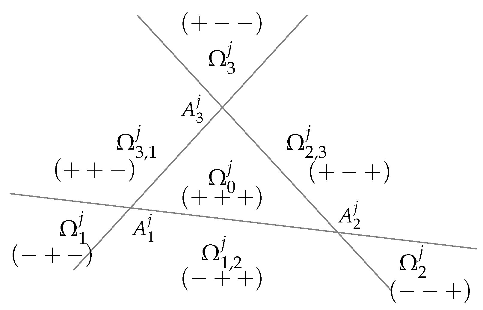
• Choose an interior point $Z_j$ in each triangle $T_j$. If two triangles $T_i$ and $T_j$ have a common edge, then the line joining $Z_i$ and $Z_j$ should intersect the common edge at some point $R_{ij}$.
• Join each point $Z_j$ to the vertices of $T_j$.
• For each edge of the triangle $T_j$:

  (a)

  which is common to a triangle $T_i$, join $Z_j$ to $R_{ij}$;

  (b)

  which belongs to the boundary $\partial \mathsf{\Omega }$, join $Z_j$ to an arbitrary point on that edge.

The space of sextic piecewise polynomials on ${\mathsf{\Delta }}_{PS}$ with global $C^2$ continuity was defined as:

$$S_6^2\left(\mathsf{\Omega },{\mathsf{\Delta }}_{PS}\right):=\left\{s\in C^2\left(\mathsf{\Omega }\right):s_{|t}\in {\mathbb{P}}_6\mathrm{for}\mathrm{all}\mathrm{micro-triangle}t\in {\mathsf{\Delta }}_{PS}\right\}.$$

This kind of spline space can be considered as the Hermitian finite element [30]. Then, we considered a particular subspace of $S_6^2\left(\mathsf{\Omega },{\mathsf{\Delta }}_{PS}\right)$ introduced in [26]. Let $\mathcal{V}:={\left\{V_i\right\}}_{i=1}^{nv}$, $\mathcal{Z}:={\left\{Z_i\right\}}_{i=1}^{nt}$ and ${\mathcal{E}}^{*}$ be, respectively, the subsets of vertices in $\mathsf{\Delta }$, split points in ${\mathsf{\Delta }}_{PS}$, and edges in ${\mathsf{\Delta }}_{PS}$ that connect a split point $Z_i$ to a point $R_{ij}$. As given in [26], the space of PS splines is defined as

$$S_6^{2,4,3}\left(\mathsf{\Omega },{\mathsf{\Delta }}_{PS}\right):=\left\{s\in S_6^2\left(\mathsf{\Omega },{\mathsf{\Delta }}_{PS}\right):s\in C^4\left(\mathcal{V}\right),s\in C^3\left(\mathcal{Z}\cup {\mathcal{E}}^{*}\right)\right\}.$$

Each $C^2\left(\mathsf{\Omega }\right)$ function s is of class $C^4$ at any vertex in $\mathcal{V}$ and of class $C^3$ at any split point in $\mathcal{Z}$ and across any edge in ${\mathcal{E}}^{*}$. In [26], by using minimal determining sets, it was proved that for given values $f_i^{a,b}$, $i=1,\dots ,nv$, and $g_k$, $k=1,\dots ,nt$, there exists a unique spline $s\in S_6^{2,4,3}\left(\mathsf{\Omega },{\mathsf{\Delta }}_{PS}\right)$ such that

$${\partial }_{a,b}s\left(V_i\right)=f_i^{a,b},0\le a+b\le 4,\mathrm{and}s\left(Z_k\right)=g_k.$$

(3)

Therefore, the dimension of the space $S_6^{2,4,3}\left(\mathsf{\Omega },{\mathsf{\Delta }}_{PS}\right)$ was equal to $15nv+nt$.

A procedure for the construction of a normalized basis for the space $S_6^{2,4,3}\left(\mathsf{\Omega },{\mathsf{\Delta }}_{PS}\right)$ was then based on the solution of the above Hermite interpolation problem for appropriate values $f_i^{a,b}$ and $g_k$ (see [26]). Non-negative and locally supported basis functions ${\mathcal{B}}_{i,j}^v$ and ${\mathcal{B}}_k^t$ with respect to vertices and triangles, respectively, that form a partition of unity were defined, and any $s\in S_6^{2,4,3}\left(\mathsf{\Omega },{\mathsf{\Delta }}_{PS}\right)$ could be represented as

$$s(x,y):=\sum _{i=1}^{nv}\sum _{j=1}^{15}{c}_{i,j}^v{\mathcal{B}}_{i,j}^v\left(x,y\right)+\sum _{k=1}^{nt}{c}_k^t{\mathcal{B}}_k^t\left(x,y\right).$$

(4)

In what follows, we gave a fully elaborate construction of such a normalized basis [25,26]. For every vertex $V_i$, let $M_i:={\cup }_{T\in \mathsf{\Delta },V_i\in T}T$ be the molecule of vertex $V_i$, i.e., the union of all triangles in $\mathsf{\Delta }$ containing $V_i$. For all vertices $V_{\ell }$, $\ell \in {\mathsf{\Lambda }}_i$ (e.g., ${\mathsf{\Lambda }}_i$ is the set of indices for the vertices that form an edge in $\mathsf{\Delta }$ with $V_i$), lying on the boundary of $M_i$, let

$$S_{i,\ell }:=\frac{1}{3}{V}_i+\frac{2}{3}{V}_{\ell }.$$

The points $V_i$ and $S_{i,\ell }$, $\ell \in {\mathsf{\Lambda }}_i$, were stated to be PS6 points associated with the vertex $V_i$. Let $t_i:=\left(Q_{i,1},Q_{i,2},Q_{i,3}\right)$ be a triangle containing the PS6 points of $V_i$. It will be called the PS6 triangle. Denote by ${\mathfrak{B}}_{t_i,mnl}^4$, $m+n+l=4$, the Bernstein polynomials of degree four with respect to $t_i$, and define, for all $0\le a+b\le 4$, the values

$$\begin{array}{cc}\hfill {\alpha }_{i,1}^{a,b}& :=C_{a,b}{\partial }_{a,b}{\mathfrak{B}}_{t_i,400}^4\left(V_i\right),{\alpha }_{i,2}^{a,b}:=C_{a,b}{\partial }_{a,b}{\mathfrak{B}}_{t_i,310}^4\left(V_i\right),{\alpha }_{i,3}^{a,b}:=C_{a,b}{\partial }_{a,b}{\mathfrak{B}}_{t_i,220}^4\left(V_i\right),\hfill \\ \hfill {\alpha }_{i,4}^{a,b}& :=C_{a,b}{\partial }_{a,b}{\mathfrak{B}}_{t_i,130}^4\left(V_i\right),{\alpha }_{i,5}^{a,b}:=C_{a,b}{\partial }_{a,b}{\mathfrak{B}}_{t_i,040}^4\left(V_i\right),{\alpha }_{i,6}^{a,b}:=C_{a,b}{\partial }_{a,b}{\mathfrak{B}}_{t_i,031}^4\left(V_i\right),\hfill \\ \hfill {\alpha }_{i,7}^{a,b}& :=C_{a,b}{\partial }_{a,b}{\mathfrak{B}}_{t_i,022}^4\left(V_i\right),{\alpha }_{i,8}^{a,b}:=C_{a,b}{\partial }_{a,b}{\mathfrak{B}}_{t_i,013}^4\left(V_i\right),{\alpha }_{i,9}^{a,b}:=C_{a,b}{\partial }_{a,b}{\mathfrak{B}}_{t_i,004}^4\left(V_i\right),\hfill \\ \hfill {\alpha }_{i,10}^{a,b}& :=C_{a,b}{\partial }_{a,b}{\mathfrak{B}}_{t_i,103}^4\left(V_i\right),{\alpha }_{i,11}^{a,b}:=C_{a,b}{\partial }_{a,b}{\mathfrak{B}}_{t_i,202}^4\left(V_i\right),{\alpha }_{i,12}^{a,b}:=C_{a,b}{\partial }_{a,b}{\mathfrak{B}}_{t_i,301}^4\left(V_i\right),\hfill \\ \hfill {\alpha }_{i,13}^{a,b}& :=C_{a,b}{\partial }_{a,b}{\mathfrak{B}}_{t_i,211}^4\left(V_i\right),{\alpha }_{i,14}^{a,b}:=C_{a,b}{\partial }_{a,b}{\mathfrak{B}}_{t_i,121}^4\left(V_i\right),{\alpha }_{i,15}^{a,b}:=C_{a,b}{\partial }_{a,b}{\mathfrak{B}}_{t_i,112}^4\left(V_i\right),\hfill \end{array}$$

(5)

with $C_{a,b}:=\frac{30}{\left(6-a-b\right)\left(5-a-b\right)}{\left(\frac{2}{3}\right)}^{a+b}$.

They are used to define the B-splines ${\mathcal{B}}_{i,j}^v$ and ${\mathcal{B}}_k^t$ as follows.

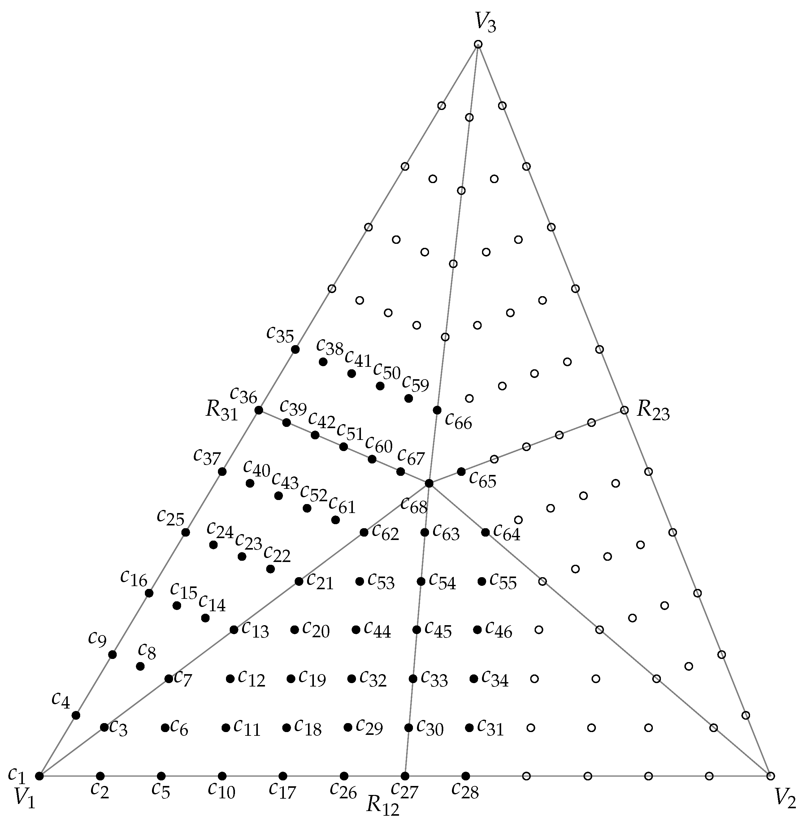
3.1. Vertex B-Spline

Every B-spline ${\mathcal{B}}_{i,j}^v$, $1\le j\le 15$, relative to the vertex $V_i$ was defined as the unique solution of a particular Hermite interpolation with conditions given by (3). Firstly, all $f_{\ell }^{a,b}$ were equal to zero except for $\ell =i$, and $f_i^{a,b}={\alpha }_{i,j}^{a,b}$. Moreover, if $V_i$ was a vertex of a triangle $T_k:=⟨V_1,V_2,V_3⟩$, then $g_k$ was equal to a value ${\beta }_{i,j}^k$ to be precise later and the remaining   values of g were all equal to zero. The spline defined in this way was zero outside the molecule $M_i$ of vertex $V_i$. Next, we computed the BB-coefficients of ${\mathcal{B}}_{i,j}^v$ relative to the triangles determining their support. For the sake of simplicity, we only computed the BB-coefficients of the B-spline ${\mathcal{B}}_{1,j}^v$ relative to the vertex $V_1$ of triangle $T_k$. The corresponding Bézier ordinates are schematically represented in Figure 3.

Figure 3. Representation of the Bézier ordinates of a B-spline relative to a vertex. The BB-coefficients that are known to be zero are indicated by open ∘.

From the definition of ${\mathcal{B}}_{1,j}^v$, many BB-coefficients were equal to zero. Figure 4 shows the refinement of $T_k$ and we assumed that the points indicated in the figure had the following barycentric coordinates:

$$\begin{array}{cc}\hfill V_1& =(1,0,0),V_2=(0,1,0),V_3=(0,0,1),Z=(z_1,z_2,z_3),\hfill \\ \hfill R_{12}& =({\lambda }_{12},{\lambda }_{21},0),R_{23}=(0,{\lambda }_{23},{\lambda }_{32}),R_{31}=({\lambda }_{13},0,{\lambda }_{31}).\hfill \end{array}$$

Because of the $C^4$ smoothness of the spline at $V_1$, the ordinates $c_1,c_2,\dots ,c_{25}$ were uniquely determined by the values ${\alpha }_{1,j}^{a,b}$, $0\le a+b\le 4$. The ordinates $c_{26},\dots ,c_{34}$ were obtained by the $C^3$ smoothness across the edge $⟨R_{12},Z⟩$.

Figure 4. A Powell–Sabin split of the triangle $T=⟨V_1,V_2,V_3⟩$.

Let us define three univariate cubic polynomial functions $p_3^0$, $p_3^1$ and $p_3^2$ on the segments $⟨\frac{V_1+R_{12}}{2}\frac{V_2+R_{12}}{2}⟩$, $⟨\frac{3V_1+2R_{12}+Z}{6}\frac{3V_2+2R_{12}+Z}{6}⟩$ and $⟨\frac{3V_1+R_{12}+2Z}{6}\frac{3V_2+R_{12}+2Z}{6}⟩$, respectively. Before subdivision, their BB-coefficients were

$$\begin{array}{cc}\hfill b_{30}^0& =c_{10},b_{21}^0={\widehat{c}}_{17},b_{12}^0=0,b_{03}^0=0,\hfill \\ \hfill b_{30}^1& =c_{11},b_{21}^1={\widehat{c}}_{18},b_{12}^1=0,b_{03}^1=0,\hfill \\ \hfill b_{30}^2& =c_{12},b_{21}^2={\widehat{c}}_{19},b_{12}^2=0,b_{03}^2=0,\hfill \end{array}$$

respectively, where

$${\widehat{c}}_{17}=\frac{c_{17}-{\lambda }_{12}{c}_{10}}{{\lambda }_{21}},{\widehat{c}}_{18}=\frac{c_{18}-{\lambda }_{12}{c}_{11}}{{\lambda }_{21}},{\widehat{c}}_{19}=\frac{c_{19}-{\lambda }_{12}{c}_{12}}{{\lambda }_{21}}.$$

Therefore, we obtained

$$\begin{array}{cc}\hfill c_{26}& ={\lambda }_{12}(c_{17}+{\lambda }_{21}{\widehat{c}}_{17}),c_{27}={\lambda }_{12}^2(c_{17}+2{\lambda }_{21}{\widehat{c}}_{17}),c_{28}={\lambda }_{12}^2{\widehat{c}}_{17},\hfill \\ \hfill c_{29}& ={\lambda }_{12}(c_{18}+{\lambda }_{21}{\widehat{c}}_{18}),c_{30}={\lambda }_{12}^2(c_{18}+2{\lambda }_{21}{\widehat{c}}_{18}),c_{31}={\lambda }_{12}^2{\widehat{c}}_{18},\hfill \\ \hfill c_{32}& ={\lambda }_{12}(c_{19}+{\lambda }_{21}{\widehat{c}}_{19}),c_{33}={\lambda }_{12}^2(c_{19}+2{\lambda }_{21}{\widehat{c}}_{19}),c_{34}={\lambda }_{12}^2{\widehat{c}}_{19}.\hfill \end{array}$$

The values $c_{35},\dots ,c_{43}$ were determined using a similar method. They were given by the following expressions:

$$\begin{array}{cc}\hfill c_{37}& ={\lambda }_{13}(c_{25}+{\lambda }_{31}{\widehat{c}}_{25}),c_{36}={\lambda }_{13}^2(c_{25}+2{\lambda }_{31}{\widehat{c}}_{25}),c_{35}={\lambda }_{13}^2{\widehat{c}}_{25},\hfill \\ \hfill c_{40}& ={\lambda }_{13}(c_{24}+{\lambda }_{31}{\widehat{c}}_{24}),c_{39}={\lambda }_{13}^2(c_{24}+2{\lambda }_{31}{\widehat{c}}_{24}),c_{38}={\lambda }_{13}^2{\widehat{c}}_{24},\hfill \\ \hfill c_{43}& ={\lambda }_{13}(c_{23}+{\lambda }_{31}{\widehat{c}}_{23}),c_{42}={\lambda }_{13}^2(c_{23}+2{\lambda }_{31}{\widehat{c}}_{23}),c_{41}={\lambda }_{13}^2{\widehat{c}}_{23},\hfill \end{array}$$

with

$${\widehat{c}}_{25}=\frac{c_{25}-{\lambda }_{13}{c}_{16}}{{\lambda }_{31}},{\widehat{c}}_{24}=\frac{c_{24}-{\lambda }_{13}{c}_{15}}{{\lambda }_{31}},{\widehat{c}}_{23}=\frac{c_{23}-{\lambda }_{13}{c}_{14}}{{\lambda }_{31}}.$$

The remaining Bézier ordinates had to be chosen in such a way that the B-spline was $C^3$ continuous at split point Z. Therefore, let us first define the points

$$w_i:={\displaystyle \frac{V_i+Z}{2}},i=1,2,3,$$

(6)

and let $p_3\in {\mathbb{P}}_3$ be the polynomial of degree 3 defined over the triangle $T=⟨w_1,w_2,w_3⟩$ with ordinates

$$b_{300}=c_{13},b_{210}={\widehat{c}}_{20},b_{201}={\widehat{c}}_{22},b_{120}=b_{030}=b_{021}=b_{012}=b_{003}=b_{102}=b_{111}=0,$$

where

$${\widehat{c}}_{20}={\displaystyle \frac{c_{20}-{\lambda }_{12}{c}_{13}}{{\lambda }_{21}}},{\widehat{c}}_{22}={\displaystyle \frac{c_{22}-{\lambda }_{13}{c}_{13}}{{\lambda }_{31}}}.$$

(7)

We obtained

$$\begin{array}{cc}\hfill c_{44}& ={\lambda }_{12}^2{c}_{13}+2{\lambda }_{12}{\lambda }_{21}{\widehat{c}}_{20},c_{45}=12{\lambda }^3{c}_{13}+3{\lambda }_{12}^2{\lambda }_{21}{\widehat{c}}_{20},c_{46}={\lambda }_{12}^2{\widehat{c}}_{20},\hfill \\ \hfill c_{47}& =0,c_{48}=0,c_{49}=0,c_{50}={\lambda }_{13}^2{\widehat{c}}_{22},c_{51}={\lambda }_{13}^3{c}_{13}+3{\lambda }_{13}^2{\lambda }_{31}{\widehat{c}}_{22},\hfill \\ \hfill c_{52}& ={\lambda }_{13}^2{c}_{13}+2{\lambda }_{13}{\lambda }_{31}{\widehat{c}}_{22},c_{53}=z_1{\lambda }_{12}{c}_{13}+(z_2{\lambda }_{12}+z_1{\lambda }_{21}){\widehat{c}}_{20}+z_3{\lambda }_{12}{\widehat{c}}_{22},\hfill \\ \hfill c_{54}& =z_1{\lambda }_{12}^2{c}_{13}+(z_2{\lambda }_{12}^2+z_1{\lambda }_{12}{\lambda }_{21}){\widehat{c}}_{20}+z_3{\lambda }_{12}^2{\widehat{c}}_{22},c_{55}={\lambda }_{12}{z}_1{\widehat{c}}_{20},c_{56}=0,\hfill \\ \hfill c_{57}& =0,c_{58}=0,c_{59}={\lambda }_{13}{z}_1{\widehat{c}}_{22},c_{60}=z_1{\lambda }_{13}^2{c}_{13}+z_2{\lambda }_{13}^2{\widehat{c}}_{20}+(z_3{\lambda }_{13}^2+2z_1{\lambda }_{13}{\lambda }_{31}){\widehat{c}}_{22},\hfill \\ \hfill c_{61}& =z_1{\lambda }_{13}{c}_{13}+z_2{\lambda }_{13}{\widehat{c}}_{20}+(z_3{\lambda }_{13}+z_1{\lambda }_{31}){\widehat{c}}_{22},c_{62}=z_1^2{c}_{13}+2z_1{z}_2{\widehat{c}}_{20}+2z_1{z}_3{\widehat{c}}_{22},\hfill \\ \hfill c_{63}& =z_1^2{\lambda }_{12}{c}_{13}+(2z_1{z}_2{\lambda }_{12}+z_1^2{\lambda }_{21}){\widehat{c}}_{20}+2z_1{z}_3{\lambda }_{12}{\widehat{c}}_{22},c_{64}=z_1^2{\widehat{c}}_{20}+2z_1{z}_3{\widehat{c}}_{22},\hfill \\ \hfill c_{65}& =z_1^2{\lambda }_{23}{\widehat{c}}_{20}+z_1^2{\lambda }_{32}{\widehat{c}}_{22},c_{66}=z_1^2{\widehat{c}}_{22},\hfill \\ \hfill c_{67}& =z_1^2{\lambda }_{13}{c}_{13}+2z_1{z}_2{\lambda }_{13}{\widehat{c}}_{20}+(2z_1{z}_3{\lambda }_{13}+z_1^2{\lambda }_{31}){\widehat{c}}_{22},c_{68}=z_1^3{c}_{13}+3z_1^2{z}_2{\widehat{c}}_{20}+3z_1^2{z}_3{\widehat{c}}_{22}.\hfill \end{array}$$

The choice ${\beta }_{1,j}^k=c_{68}$ provided the values needed to completely define the B-spline ${\mathcal{B}}_{1,j}^v$.

Figure 5 shows typical plots of the fifteen $C^2$ sextic B-splines associated with a vertex of the triangulation.

Figure 5. B-splines relative to a vertex.

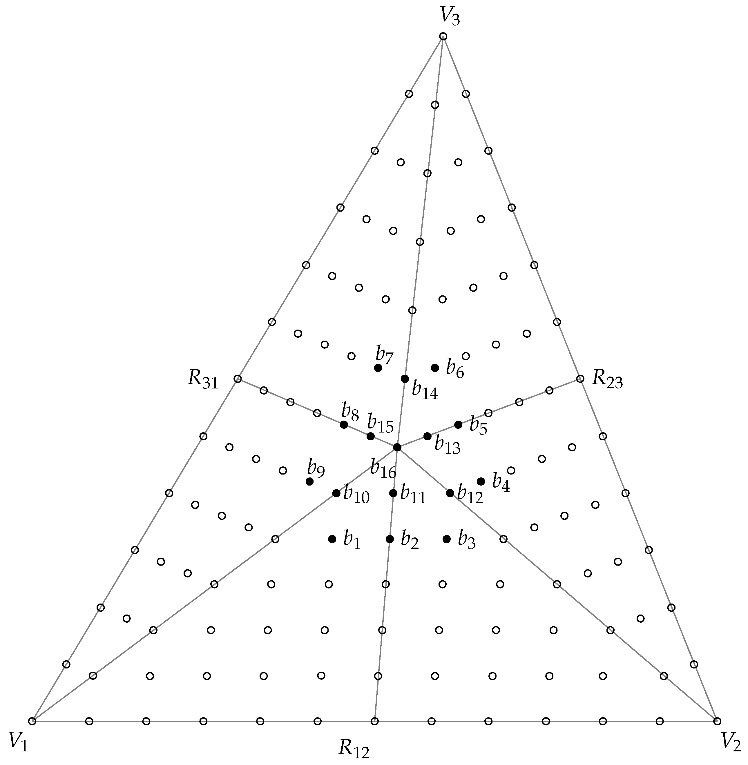
3.2. Triangle B-Spline

For the sake of simplicity, we denoted by $b_l$ the B-ordinates with respect to a triangle (see Figure 6). The B-spline ${\mathcal{B}}_k^t$ with respect to triangle $T_k$ was defined as the spline satisfying conditions (3) with all $f_i^{a,b}$ equal to zero, $g_k={\beta }_k$ and the remaining values of g equal to zero. It vanished outside $T_k$. In order to specify the value of ${\beta }_k$, we looked at the Bernstein–Bézier representation of the B-spline ${\mathcal{B}}_k^t$. We consider, again, the macro-triangle $T_k=⟨V_1,V_2,V_3⟩$, as above.

Figure 6. Schematic representation of the Bézier ordinates of a B-spline with respect to a triangle. The B-coefficients that are known to be zero are indicated by open ∘.

Let us define again a polynomial $p_3\in {\mathbb{P}}_3$ of degree 3 defined on the triangle $T=⟨w_1,w_2,w_3⟩$, where $w_i$ were defined in (6), and having the following B-ordinates:

$$b_{300}=b_{210}=b_{201}=b_{120}=b_{030}=b_{021}=b_{012}=b_{003}=b_{102}=0,b_{111}=1.$$

Furthermore, as in the above subsection, we obtained

$$\begin{array}{cc}\hfill b_1& ={\lambda }_{21}{z}_3,b_2=2{\lambda }_{12}{\lambda }_{21}{z}_3,b_3={\lambda }_{12}{z}_3,b_4={\lambda }_{32}{z}_1,b_5=2{\lambda }_{23}{\lambda }_{32}{z}_1,b_6={\lambda }_{23}{z}_1,\hfill \\ \hfill b_7& ={\lambda }_{13}{z}_2,b_8=2{\lambda }_{13}{\lambda }_{31}{z}_2,b_9={\lambda }_{31}{z}_2,b_{10}=2z_2{z}_3,b_{11}=2z_3({\lambda }_{12}{z}_2+{\lambda }_{21}{z}_1),\hfill \\ \hfill b_{12}& =2z_1{z}_3,b_{13}=2z_1({\lambda }_{23}{z}_3+{\lambda }_{32}{z}_2),b_{14}=2z_2{z}_1,b_{15}=2z_2({\lambda }_{31}{z}_1+{\lambda }_{13}{z}_3),\hfill \\ \hfill b_{16}& =6z_1{z}_2{z}_3.\hfill \end{array}$$

(8)

From the construction, it was clear that all the Bézier ordinates were non-negative. Then, the B-spline ${\mathcal{B}}_k^t$ was non-negative. We could choose ${\beta }_k=6z_1{z}_2{z}_3$.

For each vertex $V_i$ and each triangle $T_k$, we defined points $Q_{i,\beta }:=\left(X_{i,\beta },Y_{i,\beta }\right)$ with $\beta :=\left({\beta }_1,{\beta }_2,{\beta }_3\right)$, $\left|\beta \right|:={\beta }_1+{\beta }_2+{\beta }_3=4$ and $Q_k^t:=\left(X_k^t,Y_k^t\right)$ in such a way that the reproduction of the monomials x and y held, i.e.,

$$\begin{array}{cc}\hfill \sum _{i=1}^{nv}\sum _{\left|\beta \right|=4}{X}_{i,\beta }{\mathcal{B}}_{i,\beta }^v\left(x,y\right)+\sum _{k=1}^{nt}{X}_k^t{\mathcal{B}}_k^t\left(x,y\right)& =x,\hfill \end{array}$$

(9)

$$\begin{array}{cc}\hfill \sum _{i=1}^{nv}\sum _{\left|\beta \right|=4}{Y}_{i,\beta }{\mathcal{B}}_{i,\beta }^v\left(x,y\right)+\sum _{k=1}^{nt}{Y}_k^t{\mathcal{B}}_k^t\left(x,y\right)& =y.\hfill \end{array}$$

(10)

Proposition 2.

Let$Q_{i,(4,0,0)}$,$Q_{i,(0,4,0)}$and$Q_{i,(0,0,4)}$be the three vertices of a triangle$t_i$. If the remaining points are defined by

$$Q_{i,\beta }:=\frac{1}{4}({\beta }_1{Q}_{i,(4,0,0)}+{\beta }_2{Q}_{i,(0,4,0)}+{\beta }_3{Q}_{i,(0,0,4)})$$

and

$$Q_k^t=\frac{V_1+V_2+V_3}{6}+\frac{Z_k}{2},$$

then (9) and (10) hold.

Proof. 

For all $\left(x,y\right)\in t_i$, we had

$$x=\sum _{\left|\beta \right|=4}\mathbf{B}\left[x\right]\left(Q_{i,(4,0,0)}^{{\beta }_1},Q_{i,(0,4,0)}^{{\beta }_2},Q_{i,(0,0,4)}^{{\beta }_3}\right){\mathfrak{B}}_{t_i,\beta }^4\left(x,y\right).$$

(11)

Using  (5) and  (11), we obtained (9). Now, to prove (10), we needed to show that

$$\sum _{i=1}^3\sum _{\left|\beta \right|=4}{X}_{i,\beta }{\mathcal{B}}_{i,\beta }^v\left(x,y\right)+X_k^t{\mathcal{B}}_k^t\left(x,y\right)=z_1{x}_1+z_2{x}_2+z_3{x}_3.$$

(12)

Recall that, in the construction of B-splines in the above section, the value of a PS6 spline at a split point Z was computed through a particular cubic polynomial evaluated at the split point. We considered again the macro-triangle $T_k=⟨V_1,V_2,V_3⟩$. The two cubic polynomials corresponding to the two PS6 splines in the equations (9) and (10) were denoted by $p_{x,3}\left(\tau \right)$ and $p_{y,3}\left(\tau \right)$. They were defined on the triangle with the vertices given in (6). The Bézier ordinates of $p_{x,3}$ were given by the following expressions:

$$\begin{array}{cc}\hfill b_{300}^x& =\frac{1}{2}{x}_1+\frac{1}{2}(z_1{x}_1+z_2{x}_2+z_3{x}_3),b_{210}^x=\frac{2}{3}{b}_{300}^x+\frac{1}{3}{b}_{030}^x,b_{201}^x=\frac{2}{3}{b}_{300}^x+\frac{1}{3}{b}_{003}^x,\hfill \\ \hfill b_{030}^x& =\frac{1}{2}{x}_2+\frac{1}{2}(z_1{x}_1+z_2{x}_2+z_3{x}_3),b_{120}^x=\frac{1}{3}{b}_{300}^x+\frac{2}{3}{b}_{030}^x,b_{021}^x=\frac{2}{3}{b}_{030}^x+\frac{1}{3}{b}_{003}^x,\hfill \\ \hfill b_{003}^x& =\frac{1}{2}{x}_3+\frac{1}{2}(z_1{x}_1+z_2{x}_2+z_3{x}_3),b_{102}^x=\frac{1}{3}{b}_{300}^x+\frac{2}{3}{b}_{003}^x,b_{012}^x=\frac{1}{3}{b}_{030}^x+\frac{2}{3}{b}_{003}^x.\hfill \end{array}$$

By the definition of $Q_k^t$, it held

$$b_{111}=X_k^t=\frac{1}{3}(b_{300}^x+b_{030}^x+b_{003}^x).$$

Therefore, it was clear that $p_{x,3}\left(\tau \right)={\tau }_1{b}_{300}^x+{\tau }_2{b}_{030}^x+{\tau }_3{b}_{003}^x$, and (12) followed. Hence, (9) was proved. Equality (10) could be proved in a similar way.    □

Figure 7 shows the plot of the $C^2$ sextic B-spline associated with a triangle of the triangulation ${\mathsf{\Delta }}_{PS}$.

Figure 7. B-spline relative to a triangle.

4. Nearly Optimal PS6 Triangles

The construction of a normalized PS6 basis of $S_6^{2,4,3}\left(\mathsf{\Omega },{\mathsf{\Delta }}_{PS}\right)$ was reduced to finding a set of PS6 triangles that had to contain a number of specified points. The set of PS6 triangles was not uniquely defined for a given refinement [31]. One possibility for their construction was to calculate triangles of minimal area, the so-called optimal PS triangles introduced by P. Dierckx [19]. Computationally, this problem led to a quadratic programming problem. From a practical point of view, other choices may have been more appropriate. An alternative (and easier to implement) solution is given in [31], where the sides of the PS triangle are obtained by connecting neighboring PS-points in a suitable way. This technique was adopted and improved in [21]. A particular choice of the PS6 triangles could also simplify the treatment of boundary conditions. For quasi-interpolation (see [17]), the corners of each PS6 triangle were preferred to be chosen on edges of the triangulation.

We recalled the standard method proposed in the literature [19,20,25] to construct PS6 triangles and, then, we introduced a novel procedure.

4.1. Quadratic Programming Problem

Consider points $Q_{i,j}=(X_{i,j},Y_{i,j})$, $j=1,2,3$, yielding a PS6 triangle relative to the vertex $V_i=(x_i,y_i)$ and triplets $\left({\mathsf{\Gamma }}_{i,j},{\mathsf{\Gamma }}_{i,j}^x,{\mathsf{\Gamma }}_{i,j}^y\right)$,$j=1,2,3$, satisfying the following equality:

$$\left(\begin{array}{ccc}{\mathsf{\Gamma }}_{i,1}& {\mathsf{\Gamma }}_{i,2}& {\mathsf{\Gamma }}_{i,3}\\ {\mathsf{\Gamma }}_{i,1}^x& {\mathsf{\Gamma }}_{i,2}^x& {\mathsf{\Gamma }}_{i,3}^x\\ {\mathsf{\Gamma }}_{i,1}^y& {\mathsf{\Gamma }}_{i,2}^y& {\mathsf{\Gamma }}_{i,3}^y\end{array}\right)\left(\begin{array}{ccc}{X}_{i,1}& Y_{i,1}& 1\\ X_{i,2}& Y_{i,2}& 1\\ X_{i,3}& Y_{i,3}& 1\end{array}\right)=\left(\begin{array}{ccc}{x}_i& y_i& 1\\ 1& 0& 0\\ 0& 1& 0\end{array}\right).$$

(13)

The area of the PS6 triangle being

$$\left|\begin{array}{ccc}{X}_{i,1}& Y_{i,1}& 1\\ X_{i,2}& Y_{i,2}& 1\\ X_{i,3}& Y_{i,3}& 1\end{array}\right|={\left|\begin{array}{ccc}{\mathsf{\Gamma }}_{i,1}& {\mathsf{\Gamma }}_{i,2}& {\mathsf{\Gamma }}_{i,3}\\ {\mathsf{\Gamma }}_{i,1}^x& {\mathsf{\Gamma }}_{i,2}^x& {\mathsf{\Gamma }}_{i,3}^x\\ {\mathsf{\Gamma }}_{i,1}^y& {\mathsf{\Gamma }}_{i,2}^y& {\mathsf{\Gamma }}_{i,3}^y\end{array}\right|}^{-1}=\frac{1}{{\mathsf{\Gamma }}_{i,1}^x{\mathsf{\Gamma }}_{i,2}^y-{\mathsf{\Gamma }}_{i,1}^y{\mathsf{\Gamma }}_{i,2}^x},$$

then, maximizing the objective function ${\mathsf{\Gamma }}_{i,1}^x{\mathsf{\Gamma }}_{i,2}^y-{\mathsf{\Gamma }}_{i,1}^y{\mathsf{\Gamma }}_{i,2}^x$ is one approach to obtain a triangle of smallest area. Additional constraints are needed to obtain a PS6 triangle containing all PS6 points with respect to $V_i$.

The classical construction due to Dierckx was then summarized in the next result.

Proposition 3.

The construction of an optimal PS6 triangle$t_i$with respect to vertex$V_i$is equivalent to the following quadratic programming problem: find a set of triplets$\left({\mathsf{\Gamma }}_{i,1},{\mathsf{\Gamma }}_{i,1}^x,{\mathsf{\Gamma }}_{i,1}^y\right)$, $\left({\mathsf{\Gamma }}_{i,2},{\mathsf{\Gamma }}_{i,2}^x,{\mathsf{\Gamma }}_{i,2}^y\right)$and$\left(1-{\mathsf{\Gamma }}_{i,1}-{\mathsf{\Gamma }}_{i,2},-{\mathsf{\Gamma }}_{i,1}^x-{\mathsf{\Gamma }}_{i,2}^x,-{\mathsf{\Gamma }}_{i,1}^y-{\mathsf{\Gamma }}_{i,2}^y\right)$maximizing the objective function${\mathsf{\Gamma }}_{i,1}^x{\mathsf{\Gamma }}_{i,2}^y-{\mathsf{\Gamma }}_{i,1}^y{\mathsf{\Gamma }}_{i,2}^x$subject to the constraints

$$\begin{array}{cc}\hfill {\mathsf{\Gamma }}_{i,1}+{\mathsf{\Gamma }}_{i,2}+{\mathsf{\Gamma }}_{i,3}& =1\hfill \\ \hfill {\mathsf{\Gamma }}_{i,1}^x+{\mathsf{\Gamma }}_{i,2}^x+{\mathsf{\Gamma }}_{i,3}^x& =0\hfill \\ \hfill {\mathsf{\Gamma }}_{i,1}^y+{\mathsf{\Gamma }}_{i,2}^y+{\mathsf{\Gamma }}_{i,3}^y& =0\hfill \end{array}$$

and

$$\begin{array}{cc}\hfill & {\mathsf{\Gamma }}_{i,j}\ge 0,\hfill \\ \hfill & L_{i\ell ,j}={\mathsf{\Gamma }}_{i,1}+\frac{2}{3}\left({\mathsf{\Gamma }}_{i,j}^x\left(x_{\ell }-x_i\right)+{\mathsf{\Gamma }}_{i,j}^y\left(y_{\ell }-y_i\right)\right)\ge 0,\hfill \end{array}$$

with$j=1,2,3$and for all vertices$V_{\ell }=\left(x_{\ell },y_{\ell }\right)$lying on the boundary of the molecule$M_i$of$V_i$, where$\left({\mathsf{\Gamma }}_{i,1},{\mathsf{\Gamma }}_{i,2},{\mathsf{\Gamma }}_{i,3}\right)$and$\left(L_{i\ell ,1},L_{i\ell ,2},L_{i\ell ,3}\right)$are the barycentric coordinates with respect to PS6 triangle$t_i$of the PS6 points$V_i$and$S_{i\ell }$, respectively.

The objective function of the optimization problem can be written as $max\frac{1}{2}{x}^{T}Ax$, where

$$x^T:=\left({\mathsf{\Gamma }}_{i,1},{\mathsf{\Gamma }}_{i,2},{\mathsf{\Gamma }}_{i,1}^x,{\mathsf{\Gamma }}_{i,2}^x,{\mathsf{\Gamma }}_{i,1}^y,{\mathsf{\Gamma }}_{i,2}^y\right)\mathrm{and}A=\left(\begin{array}{cccccc}0& 0& 0& 0& 0& 0\\ 0& 0& 0& 0& 0& 0\\ 0& 0& 0& 0& 0& -1\\ 0& 0& 0& 0& 1& 0\\ 0& 0& 0& 1& 0& 0\\ 0& 0& -1& 0& 0& 0\end{array}\right).$$

The eigenvalues of the matrix A were $-1$, $-1$, 1, 1, 0 and 0, so that A was indefinite. As pointed out in [19], “since the Hessian matrix of the objective function is not negative (semi-) definite, appropriate software can only find a local maximum”. Therefore, we could not guarantee that the quadratic optimization problem has a unique solution, which led to a scenario of local solutions.

The technique for determining PS6 triangles is not unique. One option for their construction is to calculate a triangle with a minimal area. Although the quadratic program of P. Dierckx [19] produces excellent results, it can also produce PS6 triangle with quite large diameters. Therefore, in order to overcome the limitation of the above optimization problem, namely, the appearance of pre-degenerated triangles, i.e., triangles with a minimal area and long diameters which impact negatively the quality of the approximation, we proposed an algorithm yielding a PS6 triangle with a diameter as small as possible.

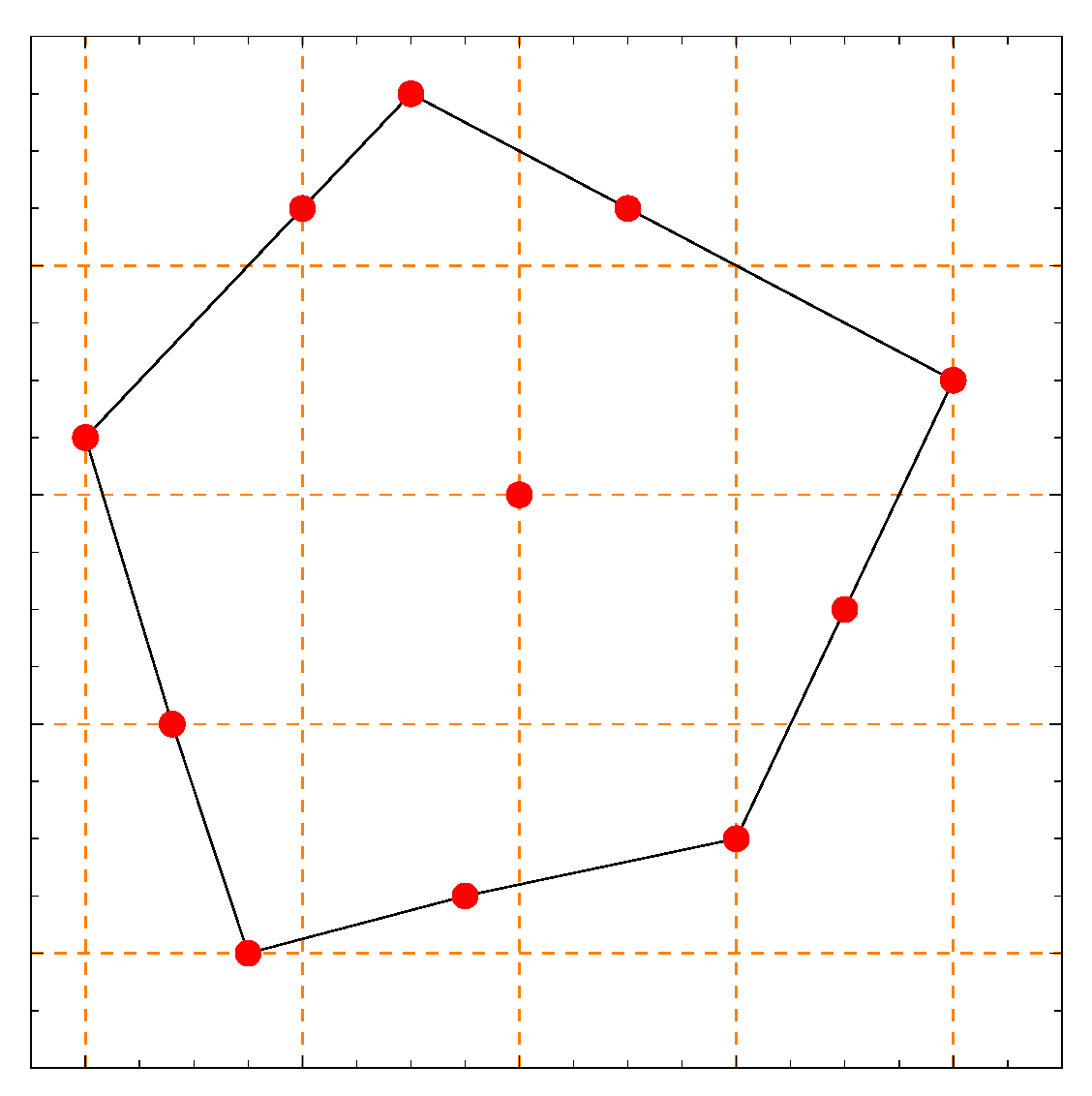
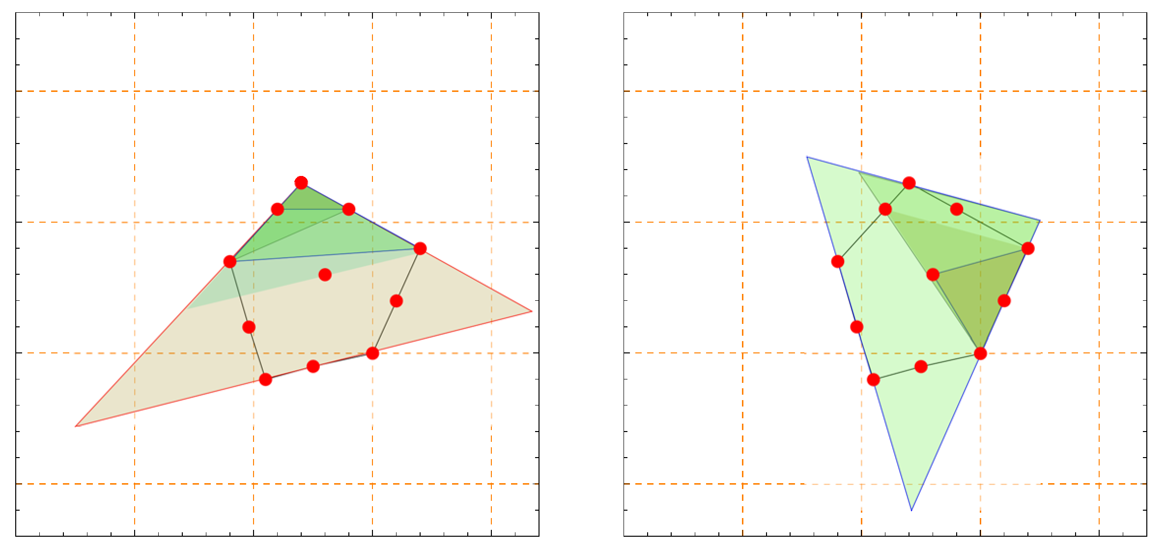
4.2. Algorithm for Determining a Triangle Containing a Set of Points

Given triangle T, let ${\left\{{\mathsf{\Omega }}_i\right\}}_{i=0}^6$ be the interiors of the seven regions obtained by extending the edges of T indefinitely (see Figure 8). Then, for each fixed $0\le i\le 6$, the barycentric coordinates of all the points in ${\mathsf{\Omega }}_i$ have constant signs. In particular, a point lies in the interior of T if and only if its barycentric coordinates are positive.

Figure 8. The seven regions determined by the triangle $T_j$, with associated signs.

The algorithm proposed here to define a triangle containing the points $A_i$, $1\le i\le n$, started from an initial triangle and built step by step triangles so that triangle $T_j:=⟨A_1^j,A_2^j,A_3^j⟩$, $j\ge 2$, obtained at the $j^{th}$ step of the algorithm contained the points $A_1$,…, $A_{j-1}$. Denote by ${\mathsf{\Omega }}_k^j$,$k=0,1,2,3$, and ${\mathsf{\Omega }}_{k,k+1}^j$,$k=1,2,3$, the seven regions obtained by dividing the plane through $T_j$ (see Figure 8).

More precisely, the procedure described in Algorithm 1 was carried out to determine a triangle from the previous one.

Figure 13 shows the PS6 triangles produced by the algorithm when applied to the PS6 points close to those used in [21]. They had two or three edges in common with the convex hull of the PS6 points.

Next, we gave a result needed to determine triangles having a nearly minimal area.

Algorithm 1Determining the triangle $T_{j+1}$ from $T_j$

Require: compute the barycentric coordinates of $A_j$ with respect to $T_j$ and select the region where $A_j$ is located.     if $A_j\in {\mathsf{\Omega }}_0^j$ then         $A_j$ is in $T_j$, perform $T_{j+1}\leftarrow T_j$ and move to the next point $A_{j+1}$     else if $A_j\in {\mathsf{\Omega }}_{3,1}^j$then Let I and J be the intersections of the line passing through $A_j$ and parallel to that passing through $\left\{A_3^j,A_1^j\right\}$ with the lines passing through $\left\{A_2^j,A_1^j\right\}$ and $\left\{A_2^j,A_3^j\right\}$, respectively, and let $T_{j+1}^1$ be the triangle with vertices $A_2^j$,$I$ and $J$. Let L be the line passing through $A_j$ and orthogonal to bisector of angle spanned by the lines $⟨A_2^j,A_1^j⟩$ and $⟨A_2^j,A_3^j⟩$. Let I and J be the intersections of L with the lines defined by $\left\{A_2^j,A_1^j\right\}$ and $\left\{A_2^j,A_3^j\right\}$, and define as $T_{j+1}^2$ the triangle with vertices $A_2^j$,$I$ and $J$. Define $T_{j+1}$ as the triangle of minimum area among $T_{j+1}^1$ and $T_{j+1}^2$.       The same process is used if $A_j$ belongs to ${\mathsf{\Omega }}_{1,2}^j$ or ${\mathsf{\Omega }}_{2,3}^j$.   else if$A_j\in {\mathsf{\Omega }}_3^j$ then       $T_{j+1}=⟨A_1^j,A_2^j,A_j⟩$.       The same procedure is applied if $A_j\in {\mathsf{\Omega }}_1^j$ or $A_j\in {\mathsf{\Omega }}_2^j$   end if

Lemma 2.

Let a,$A_1$,$A_2$,$A_3$and$A_4$be five points in${\mathbb{R}}^2$. If$a\in T_{ijk}:=⟨A_i,A_j,A_k⟩$for$i,j,k=1,2,3,4$and$i\ne j\ne k$, then, a is in the triangle obtained by applying the algorithm using$T_{ijk}$and$A_l$,$l\ne i\ne j\ne k$.

Proof. 

For the sake of simplicity, consider only one of the four different triangles which can be obtained from four points. Let $T_{134}:=⟨A_1,A_3,A_4⟩$ be a triangle containing a. By applying the algorithm proposed here to $T_{134}$ and $A_2$, we can distinguish the following scenarios:

• If $A_2\in T_{134}$, then, the resulting triangle will be $T_{134}$ itself.
• If $A_2\notin T_{134}$, then the obtained triangle will contain $T_{134}$.

In both cases the resulting triangle will contain $T_{134}$, so will contain also a. The proof is complete. □

From Lemma 2, at step j in the algorithm, we used the four triangles obtained by a permutation of the vertices of $T_j$ and $A_j$, and we chose the triangle of the small diameter among the four ones.

Figure 9 shows the PS6 triangles provided by the proposed algorithm for the considered triangulation. It can be noticed that the resulting triangles passed through at least three PS6 points. They had near minimal areas and smaller diameters.

Figure 9. A triangulation with the PS6 triangles obtained by the proposed algorithm.

As stated before, the quadratic optimization problem proposed by P. Dierckx [19] can produce PS6 triangles with quite large diameters, and the algorithm proposed here aimed to avoid this problem even though the resulting triangles had no minimal areas. Figure 10 shows the results provided by the Dierckx’s method and the algorithm for minimizing the diameter when a near degenerate vertex was considered.

Figure 10. PS6 triangles associated with a near degenerate vertex obtained by quadratic programming (a) and the proposed algorithm (b). The area of the triangle provided by the Dierckx’s method was equal to 0.2344 cm${}^2$ and the diameter was equal to 12.7857 cm. The area and the diameter of the second one were 0.25 cm${}^2$ and 7.9907 cm, respectively.

Figure 11 shows the results obtained when the time of execution of both algorithms was examined. The time required by Dierckx’ algorithm was more than 30 times longer than that required by the proposed algorithm.

Figure 11. Results produced by the proposed algorithm (a) and Dierckx’s algorithm (b).

Other algorithms for determing PS triangles have also been described in the literature. As stated before, in [21], after Proposition 1, the authors outline an algorithm that produces PS triangles sharing two or three edges with the convex hull of the PS points. Next, we compare it with our Algorithm. To conduct that, we considered PS points such as those in Figure 1 in [21]. They are represented in Figure 12.

Figure 12. PS points close to those of the ones in [21].

Algorithm 1 provided the PS6 triangles shown in Figure 13. Each of them was produced from a choice of an initial triangle. On the left side, we showed those obtained after three steps starting from the small dark triangle. We saw that these PS triangles shared two or three sides with the convex hull of the PS points. On the right side, we showed two other PS triangles produced by the algorithm after four steps. They also shared two or three sides with the convex hull. The results provided by the algorithm in [21] and Algorithm 1 were similar, although the later one did not need to compute the convex hull of the PS points.

Figure 13. Results produced by the proposed algorithm applied to a set of PS6 points close to the points indicated in Figure 12.

5. Quasi-Interpolation Schemes with Optimal Approximation Order

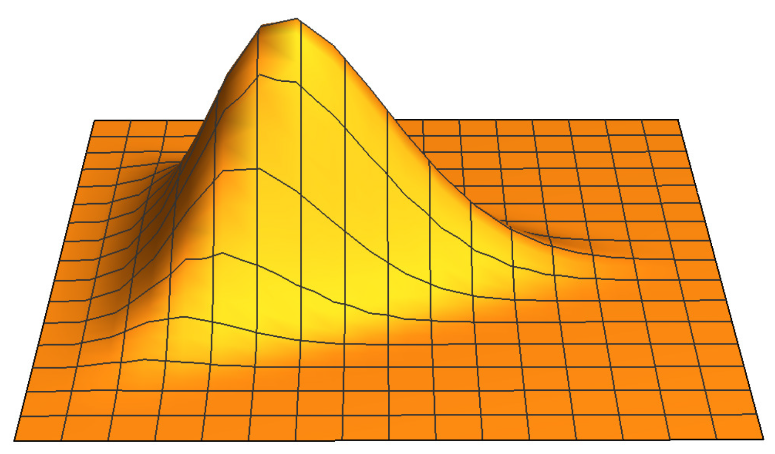
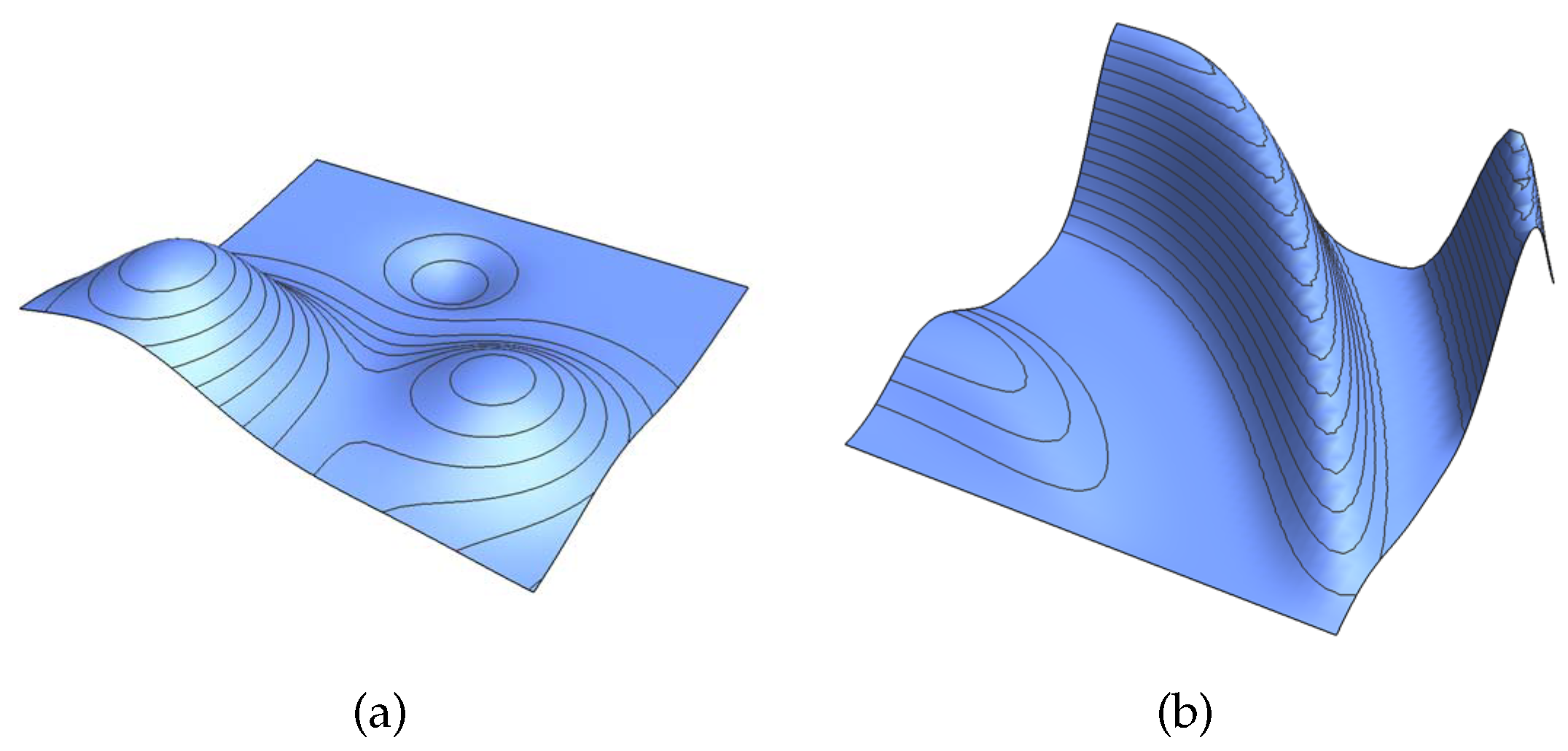
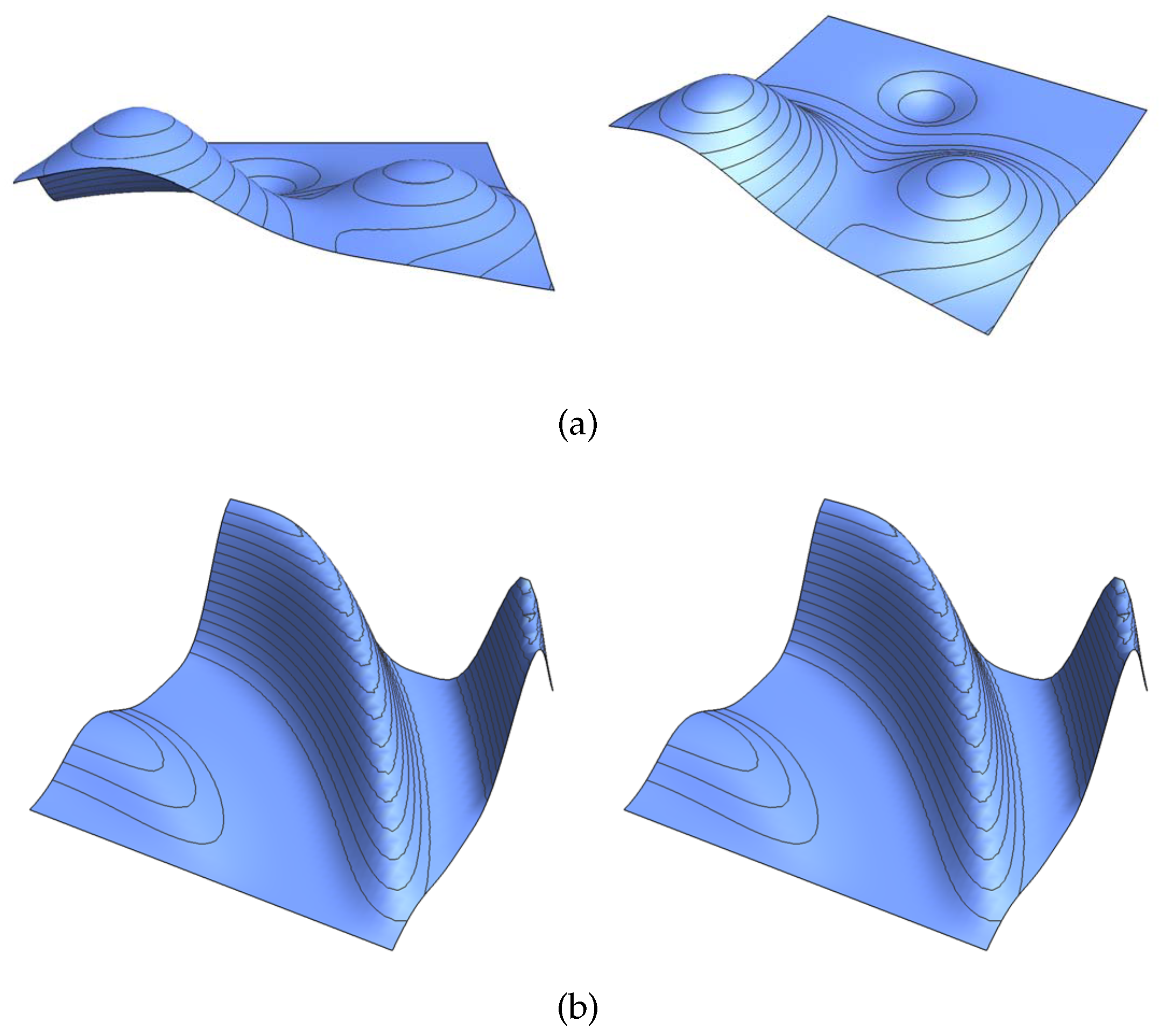
In this section, we gave proof of the Marsden’s identity for the space $S_6^{2,4,3}\left(\mathsf{\Omega },{\mathsf{\Delta }}_{PS}\right)$, expressing any spline s in this space as a linear combination of the normalized sextic Powell–Sabin B-splines defined above. The coefficients in that combination were given in terms of the polar forms of s. Therefore, Proposition 1 facilitates the establishment of Marsden’s identity in comparison with other existing methods (e.g., matrix inverse [20]).

Here, we used the same notation as in Section 3. Let $Q_{i,j},j=1,2,3$, be the vertices of a PS6 triangle $t_i$ with respect to $V_i$. Define

$${\tilde{Q}}_{i,j}:=-\frac{1}{2}{V}_i+\frac{3}{2}{Q}_{i,j},i=1,\dots ,nv,j=1,2,3.$$

We had the following result.

Corollary 1.

For any$p\in {\mathbb{P}}_6$it holds

$$p=\sum _{i=1}^{nv}\sum _{\left|\beta \right|=4}\mathbf{B}\left[p\right]\left(V_i^2,{\tilde{Q}}_{i,1}^{{\beta }_1},{\tilde{Q}}_{i,2}^{{\beta }_2},{\tilde{Q}}_{i,3}^{{\beta }_3}\right){\mathcal{B}}_{i,\beta }^v+\sum _{k=1}^{nt}\mathbf{B}\left[p\right]\left(Z_k^3,V_{k1},V_{k2},V_{k3}\right){\mathcal{B}}_k^t,$$

(14)

where$V_{k1},V_{k2}$and$V_{k3}$are the vertices of the macro triangle containing$Z_k$.

Proof. 

Define

$$s=\sum _{i=1}^{nv}\sum _{\left|\beta \right|=4}\mathbf{B}\left[p\right]\left(V_i^2,{\tilde{Q}}_{i,1}^{{\beta }_1},{\tilde{Q}}_{i,2}^{{\beta }_2},{\tilde{Q}}_{i,3}^{{\beta }_3}\right){\mathcal{B}}_{i,\beta }^v+\sum _{k=1}^{nt}\mathbf{B}\left[p\right]\left(Z_k^3,V_{k1},V_{k2},V_{k3}\right){\mathcal{B}}_k^t.$$

We proved that

$${\partial }_{a,b}s\left(V_i\right)={\partial }_{a,b}p\left(V_i\right),i=1,\dots ,nv,0\le a+b\le 4,$$

and

$$s\left(Z_k\right)=p\left(Z_k\right),k=1,\dots ,nt,$$

from which the equality $s=p$ follows.

It was clear that

$$s\left(V_i\right)=\sum _{\left|\beta \right|=4}\mathbf{B}\left[p\right]\left(V_i^2,{\tilde{Q}}_{i,1}^{{\beta }_1},{\tilde{Q}}_{i,2}^{{\beta }_2},{\tilde{Q}}_{i,3}^{{\beta }_3}\right){\mathcal{B}}_{i,\beta }^v\left(V_i\right).$$

Define

$$q_{vi}\left(X\right):=\sum _{\left|\beta \right|=4}\mathbf{B}\left[p\right]\left(V_i^2,{\tilde{Q}}_{i,1}^{{\beta }_1},{\tilde{Q}}_{i,2}^{{\beta }_2},{\tilde{Q}}_{i,3}^{{\beta }_3}\right){\mathcal{B}}_{i,\beta }^v\left(X\right).$$

From (5), for all $0\le a+b\le 4$ it held

$$\begin{array}{cc}\hfill & {\partial }_{a,b}{q}_{vi}\left(X\right)\hfill \\ \hfill & =\frac{30}{\left(6-a-b\right)\left(5-a-b\right)}{\left(\frac{4}{6}\right)}^{a+b}{\partial }_{a,b}\sum _{\left|\beta \right|=4}\mathbf{B}\left[p\right]\left(V_i^2,{\tilde{Q}}_{i,1}^{{\beta }_1},{\tilde{Q}}_{i,2}^{{\beta }_2},{\tilde{Q}}_{i,3}^{{\beta }_3}\right){\mathfrak{B}}_{t_i,\beta }^4\left(X\right)\hfill \\ \hfill & =\frac{6!}{\left(6-a-b\right)!\left(a+b\right)!}\frac{\left(a+b\right)!\left(4-a-b\right)!}{4!}{\left(\frac{4}{6}\right)}^{a+b}{\partial }_{a,b}\sum _{\left|\beta \right|=4}\mathbf{B}\left[p\right]\left(V_i^2,{\tilde{Q}}_{i,1}^{{\beta }_1},{\tilde{Q}}_{i,2}^{{\beta }_2},{\tilde{Q}}_{i,3}^{{\beta }_3}\right){\mathfrak{B}}_{t_i,\beta }^4\left(X\right).\hfill \end{array}$$

Then, we used the notion of control polynomial developed in Section 2. Let

$${\tilde{q}}_{vi}:=\mathbf{B}\left[p\right]\left(V_i^2,{\left(\frac{-1}{2}{V}_i+\frac{3}{2}X\right)}^4\right)$$

be the control polynomial of degree 4 of p at the vertex $V_i$. We could write ${\tilde{q}}_{vi}$ on the PS-triangle $t_i$ as

$${\tilde{q}}_{vi}\left(X\right)=\sum _{\left|\beta \right|=4}\mathbf{B}\left[{\tilde{q}}_{vi}\right]\left(Q_{i,1}^{{\beta }_1},Q_{i,2}^{{\beta }_2},Q_{i,3}^{{\beta }_3}\right){\mathfrak{B}}_{t_i,\beta }^4\left(X\right).$$

According to Lemma 1,

$${\tilde{q}}_{vi}\left(X\right)=\sum _{\left|\beta \right|=4}\mathbf{B}\left[p\right]\left(V_i^2,{\tilde{Q}}_{i,1}^{{\beta }_1},{\tilde{Q}}_{i,2}^{{\beta }_2},{\tilde{Q}}_{i,3}^{{\beta }_3}\right){\mathfrak{B}}_{t_i,\beta }^4\left(X\right).$$

Using Proposition 1, we deduced that

$${\partial }_{a,b}p\left(V_i\right)=\frac{30}{\left(6-a-b\right)\left(5-a-b\right)}{\left(\frac{4}{6}\right)}^{a+b}{\partial }_{a,b}{\tilde{q}}_{vi}\left(V_i\right)={\partial }_{a,b}{q}_{vi}\left(V_i\right)={\partial }_{a,b}s\left(V_i\right).$$

Then, it sufficed to prove that $s\left(Z_k\right)=p\left(Z_k\right)$. Without the loss of generality, we proved the equality only for one triangle in $\mathsf{\Delta }$. Let $T=⟨V_1,V_2,V_3⟩$ be a triangle in $\mathsf{\Delta }$ with split point $Z_1$. Then,

$$\begin{array}{cc}\hfill s\left(Z_1\right)& =\sum _{\left|\beta \right|=4}\mathbf{B}\left[p\right]\left(V_1^2,{\tilde{Q}}_{1,1}^{{\beta }_1},{\tilde{Q}}_{1,2}^{{\beta }_2},{\tilde{Q}}_{1,3}^{{\beta }_3}\right){\mathcal{B}}_{1,\beta }^v\left(Z_1\right)+\sum _{\left|\beta \right|=4}\mathbf{B}\left[p\right](V_2^2,{\tilde{Q}}_{2,1}^{{\beta }_1},{\tilde{Q}}_{2,2}^{{\beta }_2},{\tilde{Q}}_{2,3}^{{\beta }_3}){\mathcal{B}}_{2,\beta }^v\left(Z_1\right)\hfill \\ \hfill & +\sum _{\left|\beta \right|=4}\mathbf{B}\left[p\right]\left(V_3^2,{\tilde{Q}}_{3,1}^{{\beta }_1},{\tilde{Q}}_{3,2}^{{\beta }_2},{\tilde{Q}}_{3,3}^{{\beta }_3}\right){\mathcal{B}}_{3,\beta }^v\left(Z_1\right)+\mathbf{B}\left[p\right]\left(Z_1^3,V_1,V_2,V_3\right)\begin{array}{c}\hfill {\mathcal{B}}_k^t\end{array}\left(Z_1\right).\hfill \end{array}$$

From Section 3, we had

$$\begin{array}{cc}\hfill & \sum _{\left|\beta \right|=4}\mathbf{B}\left[p\right]\left(V_1^2,{\tilde{Q}}_{1,1}^{{\beta }_1},{\tilde{Q}}_{1,2}^{{\beta }_2},{\tilde{Q}}_{1,3}^{{\beta }_3}\right){\mathcal{B}}_{1,\beta }^v\left(Z_1\right)\hfill \\ \hfill & =c_{68}\hfill \\ \hfill & =z_1^3{c}_{13}+3z_1^2{z}_2{\tilde{c}}_{20}+3z_1^2{z}_3{\tilde{c}}_{22}\hfill \\ \hfill & =z_1^3\mathbf{B}\left[p\right]\left(V_1^3,Z_1^3\right)+3z_1^2{z}_2\mathbf{B}\left[p\right]\left(V_1^2,V_2,Z_1^3\right)+3z_1^2{z}_3\mathbf{B}\left[p\right]\left(V_1^2,V_3,Z_1^3\right).\hfill \end{array}$$

Similarly,

$$\begin{array}{cc}\hfill & \sum _{\left|\beta \right|=4}\mathbf{B}\left[p\right]\left(V_2^2,{\tilde{Q}}_{2,1}^{{\beta }_1},{\tilde{Q}}_{2,2}^{{\beta }_2},{\tilde{Q}}_{2,3}^{{\beta }_3}\right){\mathcal{B}}_{2,\beta }^v\left(Z_1\right)\hfill \\ \hfill & =z_2^3\mathbf{B}\left[p\right](V_2^3,Z_1^3)+3z_2^2{z}_1\mathbf{B}\left[p\right](V_2^2,V_1,Z_1^3)+3z_2^2{z}_3\mathbf{B}\left[p\right](V_2^2,V_3,Z_1^3),\hfill \\ \hfill & \sum _{\left|\beta \right|=4}\mathbf{B}\left[p\right]\left(V_3^2,{\tilde{Q}}_{3,1}^{{\beta }_1},{\tilde{Q}}_{3,2}^{{\beta }_2},{\tilde{Q}}_{3,3}^{{\beta }_3}\right){\mathcal{B}}_{3,\beta }^v\left(Z_1\right)\hfill \\ \hfill & =z_3^3\mathbf{B}\left[p\right]\left(V_3^3,Z_1^3\right)+3z_3^2{z}_1\mathbf{B}\left[p\right]\left(V_3^2,V_1,Z_1^3\right)+3z_3^2{z}_2\mathbf{B}\left[p\right]\left(V_3^2,V_2,Z_1^3\right),\hfill \end{array}$$

and

$$\mathbf{B}\left[p\right]\left(Z_1^3,V_1,V_2,V_3\right)\begin{array}{c}\hfill {\mathcal{B}}_k^t\end{array}\left(Z_1\right)=6z_1{z}_2{z}_3\mathbf{B}\left[p\right]\left(Z_1^3,V_1,V_2,V_3\right).$$

By taking into account the multi-affine property of the polar form, the claim followed. □

Then, we stated the following result, whose proof followed the idea used in [12] in dealing with quadratic Powell–Sabin splines.

Theorem 1.

For any spline$s\in S_6^{2,4,3}\left(\mathsf{\Omega },{\mathsf{\Delta }}_{PS}\right)$, it holds

$$s=\sum _{i=1}^{nv}\sum _{\left|\beta \right|=4}\mathbf{B}\left[s_i\right]\left(V_i^2,{\tilde{Q}}_{i,1}^{{\beta }_1},{\tilde{Q}}_{i,2}^{{\beta }_2},{\tilde{Q}}_{i,3}^{{\beta }_3}\right){\mathcal{B}}_{i,\beta }^v+\sum _{k=1}^{nt}\mathbf{B}\left[\begin{array}{c}\hfill {\tilde{s}}_k\end{array}\right]\left(Z_k^3,V_{k1},V_{k2},V_{k3}\right){\mathcal{B}}_k^t,$$

where$s_i:=s_{|\begin{array}{c}\hfill {\mathfrak{t}}_i\end{array}}$stands for the restriction of s to the triangle${\mathfrak{t}}_i$in${\mathsf{\Delta }}_{PS}$and${\tilde{s}}_k$is the restriction of s to a triangle$\begin{array}{c}\hfill {\mathfrak{t}}_k\end{array}=⟨V_{k1},V_{k2},V_{k3}⟩$containing$Z_k$.

Proof. 

Consider a spline s in $S_6^{2,4,3}\left(\mathsf{\Omega },{\mathsf{\Delta }}_{PS}\right)$. Let $\begin{array}{c}\hfill {\mathfrak{t}}_i\end{array}$ be a triangle in ${\mathsf{\Delta }}_{PS}$ having $V_i$ as a vertex. Let $s_i$ be the restriction of s to $\begin{array}{c}\hfill {\mathfrak{t}}_i\end{array}$, i.e., the sextic polynomial such that

$${\partial }_{a,b}s\left(V_i\right)={\partial }_{a,b}{s}_i\left(V_i\right),s\left(Z_k\right)=\begin{array}{c}\hfill {\tilde{s}}_k\end{array}\left(Z_k\right),0\le a+b\le 4.$$

Let $p_i$ be the restriction of s on $\begin{array}{c}\hfill {\mathfrak{t}}_i\end{array}$. From Corollary 1, it was clear that for all $\left(x,y\right)\in \mathsf{\Omega }$ and $r=1,\dots ,n_v$ it held

$$p_r=\sum _{i=1}^{nv}\sum _{\left|\beta \right|=4}\mathbf{B}\left[p_r\right]\left(V_i^2,{\tilde{Q}}_{i,1}^{{\beta }_1},{\tilde{Q}}_{i,2}^{{\beta }_2},{\tilde{Q}}_{i,3}^{{\beta }_3}\right){\mathcal{B}}_{i,\beta }^v+\sum _{k=1}^{nt}\mathbf{B}\left[p_r\right]\left(Z_k^3,V_{k1},V_{k2},V_{k3}\right){\mathcal{B}}_k^t.$$

Then,

$$p_r\left(V_r\right)=\sum _{\left|\beta \right|=4}\mathbf{B}\left[p_r\right]\left(V_r^2,{\tilde{Q}}_{r,1}^{{\beta }_1},{\tilde{Q}}_{r,2}^{{\beta }_2},{\tilde{Q}}_{r,3}^{{\beta }_3}\right){\mathcal{B}}_{r,\beta }^v\left(V_r\right).$$

Therefore,

$$p_r\left(V_r\right)=\sum _{\left|\beta \right|=4}\mathbf{B}\left[s_r\right]\left(V_r^2,{\tilde{Q}}_{r,1}^{{\beta }_1},{\tilde{Q}}_{r,2}^{{\beta }_2},{\tilde{Q}}_{r,3}^{{\beta }_3}\right){\mathcal{B}}_{r,\beta }^v\left(V_r\right).$$

Define,

$$q\left(x,y\right):=\sum _{i=1}^{nv}\sum _{\left|\beta \right|=4}\mathbf{B}\left[s_i\right]\left(V_i^2,{\tilde{Q}}_{i,1}^{{\beta }_1},{\tilde{Q}}_{i,2}^{{\beta }_2},{\tilde{Q}}_{i,3}^{{\beta }_3}\right){\mathcal{B}}_{i,\beta }^v\left(x,y\right)+\sum _{k=1}^{nt}\mathbf{B}\left[s_k\right]\left(Z_k^3,V_{k1},V_{k2},V_{k3}\right)\begin{array}{c}\hfill {\mathcal{B}}_k^t\end{array}\left(x,y\right).$$

It held

$$q\left(V_r\right)=\sum _{\left|\beta \right|=4}\mathbf{B}\left[s_r\right]\left(V_r^2,{\tilde{Q}}_{r,1}^{{\beta }_1},{\tilde{Q}}_{r,2}^{{\beta }_2},{\tilde{Q}}_{r,3}^{{\beta }_3}\right){\mathcal{B}}_{r,\beta }^v\left(V_r\right).$$

Then, for all $r=1,\dots ,n_v$, we obtained

$$q\left(V_r\right)=p_r\left(V_r\right)=s_r\left(V_r\right)=s\left(V_r\right).$$

Similarly, we obtained

$${\partial }_{a,b}q\left(V_r\right)={\partial }_{a,b}{p}_r\left(V_r\right)={\partial }_{a,b}{s}_r\left(V_r\right)={\partial }_{a,b}s\left(V_r\right),1\le a+b\le 4,$$

and

$$q\left(Z_k\right)=p_k\left(Z_k\right)=\begin{array}{c}\hfill {\tilde{s}}_k\end{array}\left(Z_k\right)=s\left(Z_k\right).$$

Since every element in $S_6^{2,4,3}\left(\mathsf{\Omega },{\mathsf{\Delta }}_{PS}\right)$ was uniquely determined by its values and derivative values up to order four at the vertices of $\mathsf{\Delta }$, then the claim followed and the proof was completed. □

Marsden’s identity is a useful tool for constructing quasi-interpolants to enough regular functions (see [12] and references therein for details). We used it to define differential quasi-interpolants in $S_6^{2,4,3}\left(\mathsf{\Omega },{\mathsf{\Delta }}_{PS}\right)$. Only an outline of the construction was given here.

Lef $f\in C^6\left(\mathsf{\Omega }\right)$ and $L_i^j:=\left(L_{i,x}^j,L_{i,y}^j\right)$, $i=1,\dots ,nv$, $j=1,\dots ,15$, be some fixed points lying in the union of all triangles in $\mathsf{\Delta }$ having $V_i$ as vertex. Let us suppose that they formed an unisolvent scheme in ${\mathbb{P}}_6\left({\mathbb{R}}^2\right)$, and let $p_i^j$ be the Taylor polynomial of f of degree six at $L_i^j$, i.e.,

$$p_i^j\left(x,y\right)=\sum _{0\le k+\ell \le 6}\frac{1}{k!\ell !}{\partial }_{k,\ell }f\left(L_i^j\right){\left(x-L_{i,x}^j\right)}^k{\left(y-L_{i,y}^j\right)}^l.$$

(15)

Let $p_k$ be the Taylor polynomial of degree 6 at point $L_k$ in the support of ${\mathcal{B}}_k^t$.

Define

$$\mathcal{Q}f\left(x,y\right):=\sum _{i=1}^{nv}\sum _{\left|\beta \right|=4}\mathbf{B}\left[p_i^j\right]\left(V_i^2,{\tilde{Q}}_{i,1}^{{\beta }_1},{\tilde{Q}}_{i,2}^{{\beta }_2},{\tilde{Q}}_{i,3}^{{\beta }_3}\right){\mathcal{B}}_{i,\beta }^v\left(x,y\right)+\sum _{k=1}^{nt}\mathbf{B}\left[p_k\right]\left(Z_k^3,V_{k1},V_{k2},V_{k3}\right)\begin{array}{c}\hfill {\mathcal{B}}_k^t\end{array}\left(x,y\right).$$

(16)

Let $\mathcal{Q}f$ be the quasi-interpolant defined by (16) and (15). Then, the quasi-interpolation operator $\mathcal{Q}:C^6\left(\mathsf{\Omega }\right)\to S_6^{2,4,3}\left(\mathsf{\Omega },{\mathsf{\Delta }}_{PS}\right)$ defined such that $\mathcal{Q}\left(f\right):=\mathcal{Q}f$ was exact on ${\mathbb{P}}_6$, i.e., $\mathcal{Q}\left(p\right)=p$ for all $p\in {\mathbb{P}}_6$.

Moreover, if each $L_i^j$ belonged to a triangle ${\tau }_i^j$ in ${\mathsf{\Delta }}_{PS}$ with $V_i$ as a vertex, then $\mathcal{Q}\left(s\right)=s$ for any spline $s\in S_6^{2,4,3}\left(\mathsf{\Omega },{\mathsf{\Delta }}_{PS}\right)$. Which meant that the quasi-interpolation operator $\mathcal{Q}$ was the projector.

Numerical Tests

The aim of this subsection is to test the approximation power of the proposed quasi-interpolation operator. To this end, we tested its performance using the well-known Franke and Nielson’s functions [32,33], given respectively by

$$\begin{array}{cc}\hfill f_1\left(x,y\right)& =0.75e^{-\frac{1}{4}\left({\left(9x-2\right)}^2+{\left(9y-2\right)}^2\right)}+0.75e^{\left(-\frac{1}{49}{\left(9x+1\right)}^2-\frac{1}{10}\left(9y+1\right)\right)}\hfill \\ \hfill & +0.5e^{-\frac{1}{4}\left({\left(9x-7\right)}^2+{\left(9y-3\right)}^2\right)}+0.2e^{-{\left(9x-4\right)}^2-{\left(9y-7\right)}^2}\hfill \end{array}$$

and

$$f_2\left(x,y\right)=\frac{y}{2}{cos}^4\left(4\left(x^2+y-1\right)\right),$$

whose plots appear in Figure 14.

Figure 14. Plots of the tests functions: Franke (a) and Nielson (b).

Let us consider the domain $\mathsf{\Omega }=(0,1)\times (0,1)$. The test was carried out for a sequence of a uniform mesh ${\mathsf{\Delta }}_n$ associated with the vertices $\left(ih,jh\right)$, $i,j=0,\dots ,n$, where $h:=\frac{1}{n}$. For each triangulation, we had to compute the B-splines ${\mathcal{B}}_{i,j}^v$ and ${\mathcal{B}}_k^t$ with respect to vertices and split points, respectively, and the corresponding points PS6-triangles according to the minimal area procedured described in this work.

The quasi-interpolation error was estimated as

$$\underset{\ell ,k=1,\dots ,50}{max}\left|f\left(x_{\ell },y_k\right)-\mathcal{Q}f\left(x\ell ,y_k\right)\right|,$$

where $x_i$ and $y_j$ were equally spaced points in $(0,1)$. The numerical convergence order (NCO) was given by the rate

$$NCO:={log}_2\left({\displaystyle \frac{E\left(2n\right)}{E\left(n\right)}}\right),$$

where $E\left(m\right)$ stands for the estimated error associated with ${\mathsf{\Delta }}_m$.

The estimated errors and NCOs for the functions $f_1$ and $f_2$ are shown in Table 1. They confirmed the theoretical results. Figure 15 shows two of the meshes used to define quasi-interpolants for the test functions $f_1$ and $f_2$. Figure 16 shows the plots of the splines $\mathcal{Q}{f}_1$ and $\mathcal{Q}{f}_2$ for the two above meshes.

Table 1. Estimated errors for Franke and Nielson’s functions and NCOs with $n=2^m$, $1\le m\le 3$.

		Franke’s Function		Nielson’s Function
$\mathit{n}$	$\mathit{n}$	Estimated Error	NCO	Estimated Error	NCO
2	9	$1.07\times {10}^{-1}$	–	$1.50\times {10}^{-2}$	–
4	25	$8.47\times {10}^{-4}$	$6.98$	$1.71\times {10}^{-4}$	$7.08$
8	81	$7.05\times {10}^{-6}$	$6.81$	$1.09\times {10}^{-6}$	$7.20$

Figure 15. Meshes for $n=2^m$, $1\le m\le 2$.

Figure 16. Quasi-interpolants for Franke’s function (a) and Nielson’s function (b).

6. Conclusions

In this paper, a fully carried out construction of a normalized basis of the space $S_6^{2,4,3}\left(\mathsf{\Omega },{\mathsf{\Delta }}_{PS}\right)$ introduced in [26] was given and an algorithm was proposed and compared with two others in the literature. Furthermore, an efficient manner to establish Marsden’s identity was detailed from which quasi-interpolation operators with optimal approximation order were defined. Some tests showed the good performance of these operators.

References

- Ženíšek, A. A general theorem on triangular finite C(m)-elements. Revue Française D’automatique Informatique Recherche Opérationnelle Analyse Numérique 1974, 8, 119–127. [Google Scholar] [CrossRef]
- Clough, R.W.; Tocher, J.L. Finite element stiffness matrices for analysis of plates in bending. In Proceedings of the Conference on Matrix Methods in Structural Mechanics, Wright-Patterson A. F. B., Dayton, OH, USA, 26–28 October 1965. [Google Scholar]
- Powell, M.; Sabin, M. Piecewise quadratic approximations on triangles. ACM Trans. Math. Softw. 1977, 3, 316–325. [Google Scholar] [CrossRef]
- Lamnii, A.; Lamnii, M.; Mraoui, H. A normalized basis for condensed C1 Powell-Sabin-12 splines. Comput. Aided Geom. Design. 2015, 34, 5–20. [Google Scholar] [CrossRef]
- Lai, M.J.; Schumaker, L.L. Spline Functions on Triangulations; Cambridge University Press: Cambridge, UK, 2007. [Google Scholar]
- Fortes, M.A.; González, P.; Ibxaxñez, M.J.; Pasadas, M. Interpolating minimal energy C1-Surfaces on Powell-Sabin Triangulations: Application to the resolution of elliptic problems. Numer. Methods Partial. Differ. Equ. 2014, 31, 798–821. [Google Scholar] [CrossRef]
- May, S.; Vignollet, J.; De Borst, R. Powell-Sabin B-splines and unstructured standard T-splines for the solution of the Kirchhoff-Love plate theory exploiting Bézier extraction. Int. J. Numer. Meth. Engng. 2016, 107, 205–233. [Google Scholar] [CrossRef] [Green Version]
- Chen, L.; Borst, D.R. Cohesive fracture analysis using Powell-Sabin B-splines. Int. J. Numer. Anal. Methods Geomech. 2019, 43, 625–640. [Google Scholar] [CrossRef] [PubMed] [Green Version]
- Giorgiani, G.; Guillard, H.; Nkonga, B. A Powell-Sabin finite element scheme for partial differential equations. ESAIM Proc. Surv. 2016, 53, 64–76. [Google Scholar] [CrossRef] [Green Version]
- Mulansky, B.; Schmidt, J.W. Powell-Sabin splines in range restricted interpolation of scattered data. Computing 1994, 53, 137–154. [Google Scholar] [CrossRef]
- Lamnii, M.; Mraoui, H.; Tijini, A. Raising the approximation order of multivariate quasi-interpolants. BIT Numer. Math. 2014, 54, 749–761. [Google Scholar] [CrossRef]
- Sbibih, D.; Serghini, A.; Tijini, A. Polar forms and quadratic spline quasi-interpolants on Powell Sabin partitions. Appl. Numer. Math. 2009, 59, 938–958. [Google Scholar] [CrossRef]
- Sbibih, D.; Serghini, A.; Tijini, A. Superconvergent quadratic spline quasi-interpolants on Powell-Sabin partitions. Appl. Numer. Math. 2015, 87, 74–86. [Google Scholar] [CrossRef]
- Sbibih, D.; Serghini, A.; Tijini, A. Superconvergent local quasi-interpolants based on special multivariate quadratic spline space over a refined quadrangulation. Appl. Math. Comput. 2015, 250, 145–156. [Google Scholar] [CrossRef]
- Sbibih, D.; Serghini, A.; Tijini, A.; Zidna, A. Superconvergent C1 cubic spline quasi-interpolants on Powell-Sabin partitions. BIT Numer. Math. 2015, 55, 797–821. [Google Scholar] [CrossRef]
- Remogna, S. Bivariate C2 cubic spline quasi-interpolants on uniform Powell-Sabin triangulations of a rectangular domain. Adv. Comput. Math. 2012, 36, 39–65. [Google Scholar] [CrossRef]
- Manni, C.; Sablonnière, P. Quadratic spline quasi-interpolants on Powell-Sabin partitions. Adv. Comput. Math. 2007, 26, 283–304. [Google Scholar] [CrossRef] [Green Version]
- Bartoň, M.; Kosinka, J. On numerical quadrature for C1 quadratic Powell-Sabin 6-split macro-triangles. J. Comput. Appl. Math. 2019, 349, 239–250. [Google Scholar] [CrossRef] [Green Version]
- Dierckx, P. On calculating normalized Powell-Sabin B-splines. Comput. Aided Geom. Design 1997, 15, 61–78. [Google Scholar] [CrossRef]
- Lamnii, M.; Mraoui, H.; Tijini, A.; Zidna, A. A normalized basis for C1 cubic super spline space on Powell-Sabin triangulation. Math. Comput. Simul. 2014, 99, 108–124. [Google Scholar] [CrossRef]
- Speleers, H.; Manni, C.; Pelosi, F.; Sampoli, M.L. Isogeometric analysis with Powell–Sabin splines for advection–diffusion–reaction problems. Comput. Methods Appl. Mech. Eng. 2012, 221–222, 132–148. [Google Scholar] [CrossRef]
- Grošelj, J.; Krajnc, M. C1 cubic splines on Powell-Sabin triangulations. Appl. Math. Comput. 2016, 272, 114–126. [Google Scholar] [CrossRef]
- Lai, M.J. On C2 quintic spline functions over triangulations of Powell-Sabin’s type. J. Comput. Appl. Math. 1996, 73, 135–155. [Google Scholar] [CrossRef] [Green Version]
- Lamnii, M.; Mraoui, H.; Tijini, A. Construction of quintic Powell-Sabin spline quasi-interpolants based on blossoming. J. Comput. Appl. Math. 2013, 250, 190–209. [Google Scholar] [CrossRef]
- Speleers, H. Construction of normalized B-splines for a family of smooth spline spaces over Powell-Sabin triangulations. Constr. Approx. 2013, 37, 41–72. [Google Scholar] [CrossRef]
- Grošelj, J. A normalized representation of super splines of arbitrary degree on Powell-Sabin triangles. BIT Numer. Math. 2016, 56, 1257–1280. [Google Scholar] [CrossRef]
- Speleers, H. A family of smooth quasi-interpolants defined over Powell-Sabin triangulations. Constr. Approx. 2015, 41, 297–324. [Google Scholar] [CrossRef]
- Ramshaw, L. Blossoming: A Connect-the-Dots Approach to Splines; Tech. Rep. 19; Digital Systems Research Center: Palo Alto, CA, USA, 1987. [Google Scholar]
- Seidel, H. An introduction to polar forms. IEEE Comput. Graph. Appl. 1993, 13, 38–46. [Google Scholar] [CrossRef]
- Dobronets, B.; Shaydurov, V. Hermitian Finite Element Complementing the Bogner-Fox-Schmit Rectangle Near Curvilinear Boundary. Lobachevskii J. Math. 2016, 37, 527–533. [Google Scholar] [CrossRef]
- Vanraes, E.; Dierckx, P.; Bultheel, A. On the Choice of the PS-Triangles; Technical Report 353; Department of Computer Science, K.U. Leuven: Leuven, Belgium, 2003. [Google Scholar]
- Franke, R. Scattered data interpolation: Tests of some methods. Math. Comp. 1982, 38, 181–200. [Google Scholar]
- Nielson, G.M. A first order blending method for triangles based upon cubic interpolation. Int. J. Numer. Meth. Eng. 1978, 15, 308–318. [Google Scholar] [CrossRef]
Publisher’s Note: MDPI stays neutral with regard to jurisdictional claims in published maps and institutional affiliations. |
© 2021 by the authors. Licensee MDPI, Basel, Switzerland. This article is an open access article distributed under the terms and conditions of the Creative Commons Attribution (CC BY) license (https://creativecommons.org/licenses/by/4.0/).