Algorithm Execution Time and Accuracy of NTC Thermistor-Based Temperature Measurements in Time-Critical Applications

Abstract

This paper addresses the challenges of selecting a suitable method for negative temperature coefficient (NTC) thermistor-based temperature measurement in electronic devices. Although measurement accuracy is of great importance, the temperature calculation time represents an even greater challenge since it is inherently constrained by the control algorithm executed in the microcontroller (MCU). Firstly, a simple signal conditioning circuit with the NTC thermistor is introduced, resulting in a temperature-dependent voltage U_T being connected to the MCU’s analog input. Next, a simulation-based approximation of the actual temperature vs. voltage curve is derived, resulting in four temperature notations: for a look-up table principle, polynomial approximation, B equation and Steinhart–Hart equation. Within the simulation results, the expected temperature error of individual methods is calculated, whereas in the experimental part, performed on a DC/DC converter prototype, required prework and available MCU resources are evaluated. In terms of expected accuracy, the look-up table and the Steinhart–Hart equation offer superior results over the polynomial approximation and B equation, especially in the nominal temperature range of the NTC thermistor. However, in terms of required prework, the look-up table is inferior compared to the Steinhart–Hart equation, despite the latter having far more complex mathematical functions, affecting the overall MCU algorithm execution time significantly.

1. Introduction

In power electronics, not only voltage and current but also temperature are very indicative quantities. With the measurement of the first two, the complete operation of an electronic device is controlled by means of a supervising microcontroller (MCU). With the latter, also various system quantities, i.e., root mean square (RMS) values of current and voltage, apparent and active power [1], can be calculated. Voltage and current measurements in electronic devices together with inventive circuit topologies can prevent severe malfunction, resulting in fault-tolerant devices that can still operate under a short- or open-circuit switch failure [2,3,4]. The case is similar regarding temperature measurements: they are not limited only to applications where the temperature of a technological process is monitored or controlled, as, for instance, in material science and mechanics [5], bioelectrochemistry and biomedical engineering [6,7] or microfluidics [8,9], to name just a few. Temperature measurements are also used—often in conjunction with voltage and current measurements—to monitor key components of the device in order to increase the operational safety and reliability of the device in general. A preventive monitoring based on voltage and current measurement to calculate the temperature of a power switch is reported in [10,11], whereas a direct temperature measurement was studied in [12] to prevent power switch failure and efficiency degradation.

As for the temperature measurement, there are mainly four types of sensors used in power electronics: thermocouples [13], resistance temperature detectors (RTD) such as the temperature probe PT100 as reported in [14], thermistors [15] and dedicated integrated circuits (IC) [16]. In contrast to thermocouples, being active elements, the latter three must have a source of excitation. Nevertheless, in all cases, some sort of signal conditioning circuit needs to be implemented to obtain information on temperature.

Among the four types of sensors, thermistors are the most widely used, because they offer a fast response and are cost-effective. Their usage is not limited to electronic devices only. In [17], they were used to measure the temperature profile of the ground top layer to determine the effect of weather and rainfall on the quality of the soil; moreover, in [18], they were used to study the quality of ice cover in rivers.

A distinctive feature of thermistors is the highly non-linear dependence of resistance with temperature, which is a fact to consider even with modern cutting-edge materials and manufacturing technologies [19]. To compensate for this, various approaches have been made to linearise the response—from hardware-based signal conditioning circuits to computer-based solutions or their combinations, implementing modern techniques, such as artificial neural networks [20] and field-programmable arrays (FPGA) [21,22,23]. On the hardware side, common solutions mainly rely on conditioning circuits implementing standalone operational amplifiers (OP ap) circuits [23,24] or voltage-controlled oscillators using dedicated timer ICs (555) [25,26,27], where a thermistor is connected to a frequency-determining input stage of the timing circuit, thus resulting in a more or less linear dependence of output frequency with temperature.

In this paper, a thermistor-based temperature measurement is analysed for four calculation methods from the perspective of the calculation time needed in the MCU to calculate the temperature from the measured voltage at its input. However, since all four methods rely on the approximation of the actual thermistor resistance vs. temperature, they inherently introduce a certain temperature error. The main goal of the analysis was to evaluate the amount of required prework and to find a calculation method that results in a tolerable error (i.e., maximum of ±1 °C) in the broadest temperature range possible, yet not to exceed the hardware-imposed maximum time of the control algorithm that is executed in the MCU.

The paper is organised as follows. Section 2 recaps the basics of thermistors and their resistance change with temperature. Furthermore, a simple and cost-effective signal conditioning circuit is introduced. In Section 3, a simulation-based review of four analytical methods for temperature calculation is given. The main contribution of this paper is described in Section 4, where experimental results are compared for all proposed temperature calculation routines. Additionally, the investigated approaches are evaluated in terms of their required prework, complexity, expected accuracy and, finally, required MCU resources.

2. Principle of Temperature Measurement Using NTC Thermistors

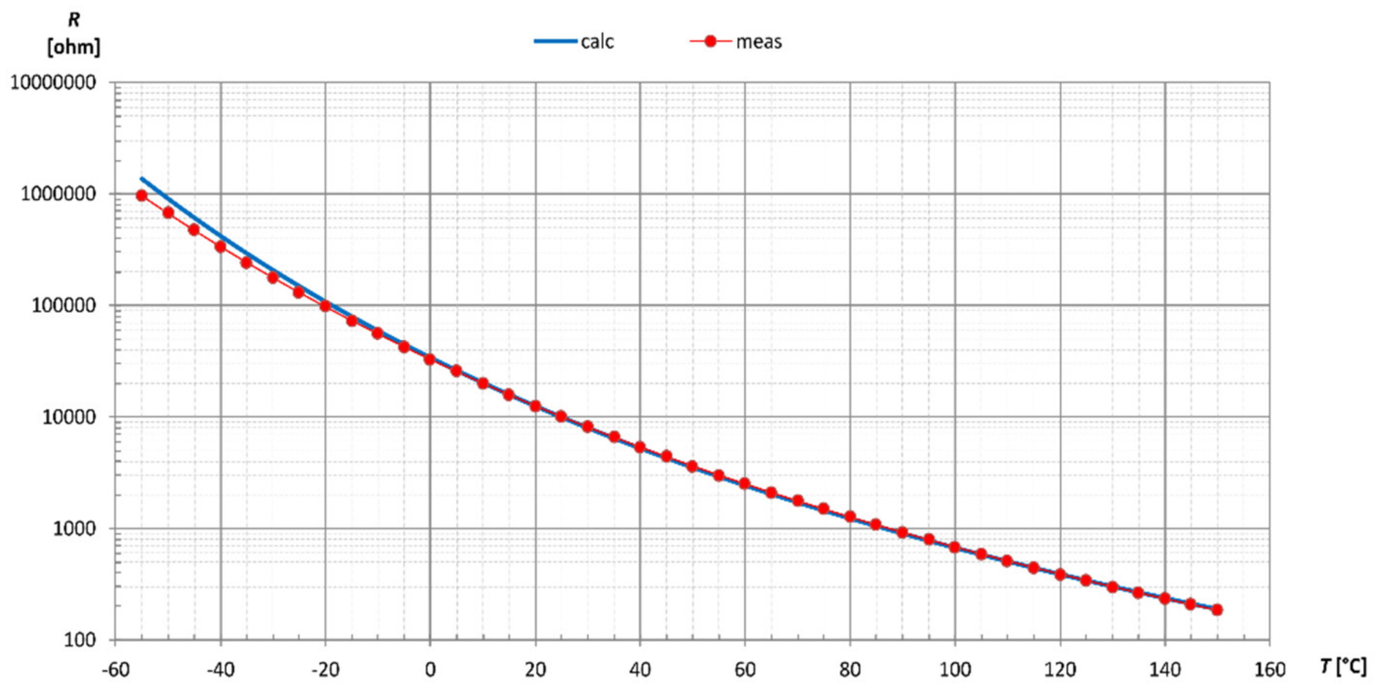
2.1. NTC Thermistor Basics

There are two types of temperature-dependent resistors (thermistors) used to detect a temperature change. With Negative Temperature Coefficient (NTC) thermistors, the resistance decreases as the temperature increases—in contrast to Positive Temperature Coefficient (PTC) thermistors. NTC thermistors are most common in cost-sensitive temperature measurements over a wide temperature range—typically between −55 °C and 150 °C [28]. Their resistance versus temperature dependence (R(T)) is highly non-linear and resembles an exponential-like function. Actual measured data R(T) are usually available in a graph or a table for a limited number of discrete temperatures and various nominal ranges. In the following text, the range between −55 °C and 150 °C is denoted as nominal. Many datasheets, in addition, offer parameters for the analytical description of R(T). The Steinhart–Hart equation [29] yields a very close match [22] with the actual measurement data in the whole nominal temperature range of the NTC thermistor:

$$\frac{1}{T}=a+b·\ln R+c·{\left(\ln R\right)}^3,$$

(1)

where T is the temperature on the Kelvin scale and a, b and c stand for Steinhart–Hart parameters. They can be provided by the thermistor manufacturer or calculated manually based on a set of three NTC resistances measured at different temperatures [30]. To find the R(T) dependence, the cubic equation for lnR in (1) should be solved, yielding in a real root

$$R=e^{\left(\sqrt[3]{y-\frac{x}{2}}-\sqrt[3]{y+\frac{x}{2}}\right)}$$

(2)

With

$$x=\frac{1}{c}\left(a-\frac{1}{T}\right) \mathrm{and}$$

(3)

$$y=\sqrt{{\left(\frac{b}{3c}\right)}^3+\frac{x^2}{4}}$$

(4)

Due to the rather complex calculation of parameters to obtain the NTC resistance from the Steinhart–Hart Equation (2), we prefer its simplified version using the B (beta) parameter

$$R=R_0·e^{B\left(\frac{1}{T}-\frac{1}{T_0}\right)}.$$

(5)

obtained after a substitution

$$\begin{gathered} a=\frac{1}{T_0}-\frac{1}{B}·\ln R_0, \\ b=\frac{1}{B} \mathrm{and} \\ c=0 \end{gathered}$$

(6)

in (1) is made. In (5), R₀ stands for the resistance at room temperature (at T₀ = 298.15 K). In contrast to the Steinhart–Hart equation, only two points on the R(T) curve are needed to calculate the possibly missing beta parameter. A general notation B_25/100 indicates that reference temperatures 25 °C and 100 °C are used to describe (5) across the nominal temperature range. Consequently, both analytical expressions (1) and (5) describe the R(T) only with a certain precision. To illustrate this, the calculated resistance R_calc of 10 kΩ thermistor EPCOS B57351V5103H060 with a B_25/100 = 4000 K [28] using (5) is compared in Figure 1 against its measured resistance R_meas, extracted and interpolated from the datasheet table.

Expressing the error

$$\Delta R\%=\frac{Rcalc-Rmeas}{Rmeas}·100\%,$$

(7)

the matching across the nominal temperature range can be even more apparent, as depicted in Figure 2 (labelled ΔR_B). The resistance error ΔR_B is zero on the B_25/100 boundaries, i.e., at 25 °C and 100 °C. Between these two values, the error never surpasses 2%. In contrast, the error becomes higher outside the B_25/100 region, especially in the low-temperature region, where the NTC thermistors exhibit immense resistance change by default. In the same figure, the resistance error for the Steinhart–Hart NTC model ΔR_SH is also plotted (secondary y-axis). It was calculated using (2–4) and (7), where the NTC resistance (2) was obtained based on the manufacturers’ datasheet [28] for resistances at temperatures −55 °C, 25 °C and 150 °C, respectively. The parameters a = 1.139357363 × 10⁻³, b = 2.327048139 × 10⁻⁴ and c = 9.134393411 × 10⁻⁸ needed in (2–4) were assessed using an online Steinhart–Hart calculator tool [31]. It is noticeable (Figure 2) that the Steinhart–Hart model is far superior to the B model in describing the NTC resistance vs. temperature. In contrast with the Steinhart–Hart parameters fitted for the whole nominal temperature range, the B_25/100-related calculation optimally describes the thermistor in the partial range from 25 °C to 100 °C only.

With a modified B value tuned for a selected temperature range of interest, as reported in [32], higher accuracy can also be achieved in a low-temperature region.

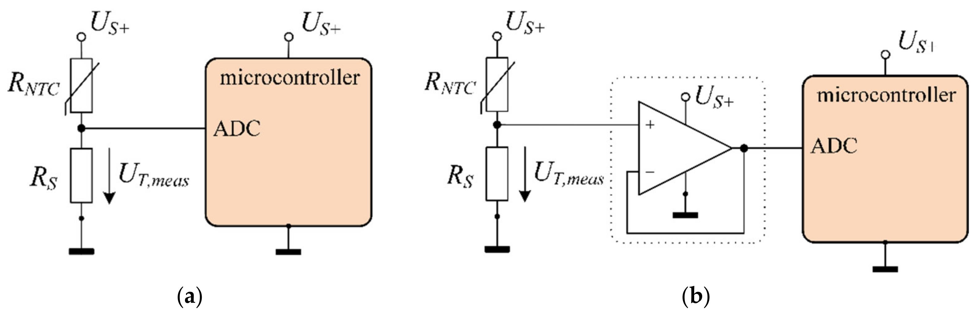
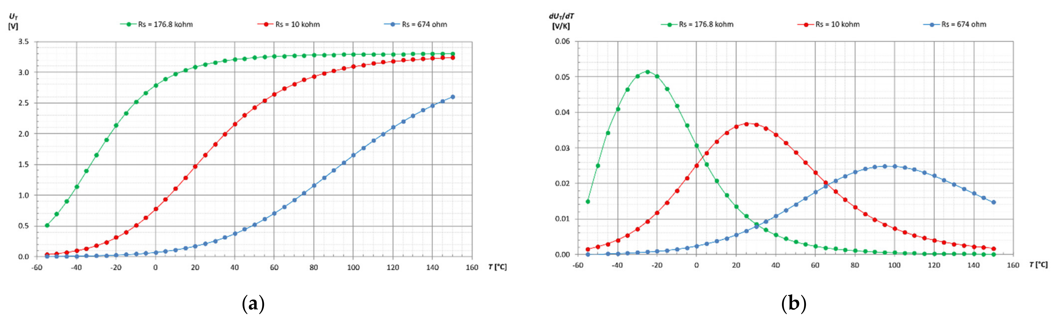
2.2. Signal Conditioning Circuit

To convert the change in NTC resistance into an equivalent voltage suitable for subsequent acquisition with an Analog–Digital Converter (ADC), the conditioning circuit is mandatory. Several types are known [33,34,35], yet the most cost-efficient version with only one additional fixed resistor (R_S), shown in Figure 3a, was selected. In our case, the voltage divider tap was directly connected to the ADC input, thus resulting in the measured voltage:

$$U_{T,meas}=U_{S+}·\frac{R_S}{R_{NTC}+R_S}.$$

(8)

For further simplification, the DC supply voltage U_S+ is considered time- and temperature-invariable. The proposed direct connection is justified if the settling time of the ADC’s sample and hold circuitry is not violated. An operational amplifier-based voltage follower inserted in front of the ADC (Figure 3b) can omit the resulting error that could more likely occur at low temperatures, i.e., high NTC resistance. Moreover, the follower is also mandatory whenever the ADC’s input resistance is comparable to the equivalent resistance formed by R_NTC and R_S. Nevertheless, the operational amplifier’s offset voltage and temperature drift could raise accuracy concerns.

The resistance R_S should be selected primarily according to the preferred temperature operating range in which maximum measurement sensitivity should occur, but also considering the supply current in order to avoid thermistor self-heating. To illustrate this, the U_T vs. temperature is plotted in Figure 4a for three values of R_S, namely 176.8 kΩ, 10 kΩ and 674 Ω, which coincide with the measured NTC resistance (Figure 1) at −30 °C, 25 °C and 100 °C, respectively. Its impact on the voltage measurement sensitivity is additionally shown in Figure 4b, assuming a supply voltage U_S+ = 3.3 V. Figure 4b reveals that sensitivity peaks for the selected values R_S at around −30 °C, 25 °C and 100 °C, respectively. The sensitivity curve flattens as its magnitude decreases, demonstrating the linearisation effect of the R_S.

3. Simulation-Based Review of Calculation Methods

Temperature measurement using NTC thermistors in an electronic device relies on a voltage measurement by means of a supervising microcontroller and its analog input circuitry. The main objective during the design stage is to find a relevant algorithm that can convert the measured voltage into its temperature equivalent. There are several ways to achieve this. Since their execution time, required prework, accuracy and adequacy to be used in the whole temperature range could differ, the methods were numerically evaluated, supposing a specimen thermistor [28,36], the proposed conditioning circuit (Figure 3) for U_S+ = 3.3 V and R_S = 10 kΩ.

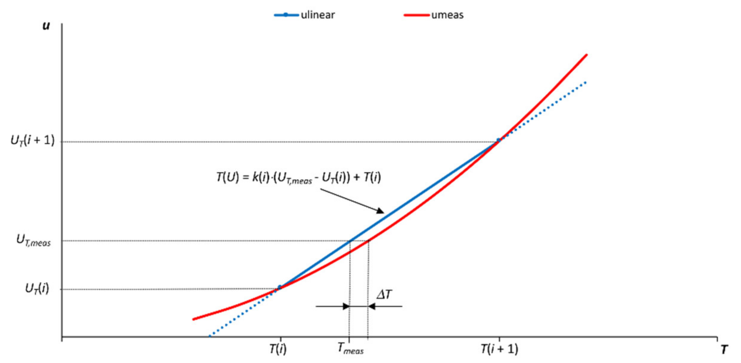
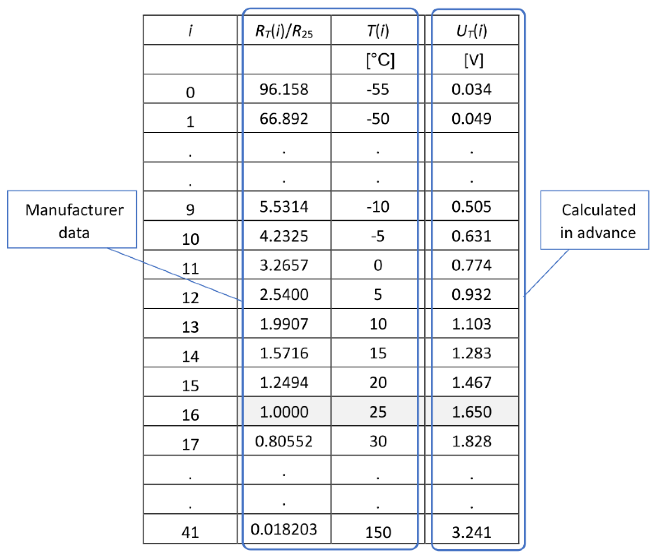
3.1. Look-Up Table with Interpolation

The look-up table principle is relatively simple but requires quite a lot of prework. A table of actual measured data R(T) provided by the manufacturer is initially subjected to indexation, forming an input array T(i) (Figure 5). Using the relation (8), an extra column with corresponding voltage equivalents U_T(i) is added.

However, since the input data are given at discrete temperatures, most commonly in 5 °C intervals, and the microcontroller memory space is also limited, intermediate values (T_meas) must be calculated by linear interpolation. In this way, a nonlinear curve defined at discrete points is converted into a set of straight lines, thus introducing a slightly more complex calculation procedure. It becomes a part of the control algorithm being executed in the microcontroller at periodic interrupts. When triggered, the algorithm checks to which interval (index i) the sampled voltage U_T,meas correlates (Figure 6):

$$U_T\left(i\right)\le U_{T,meas}\le U_T\left(i+1\right).$$

(9)

For the established index (i), two corresponding temperatures T(i) and T(i + 1) from the manufacturer’s array are picked up to calculate the slope k(i) (can be done as prework in advance) for the approximation line (labelled ulinear in Figure 6)

$$k\left(i\right)=\frac{T\left(i+1\right)-T\left(i\right)}{U_T\left(i+1\right)-U_T\left(i\right)}$$

(10)

resulting finally in the temperature equivalent T_meas calculated from the measured voltage U_T,meas

$$T_{meas}=k\left(i\right)·(U_{T,meas}-U_T\left(i\right))+T\left(i\right).$$

(11)

Figure 6. Linear interpolation principle.

Figure 6. Linear interpolation principle.

An error ΔT created by linear approximation (Figure 6) is zero only at the boundaries of each interval. Between them, the error depends on the shape of the interpolated curve based on data from the datasheet table (labelled umeas). Following (11), the implemented method exhibits a temperature error calculated for the specimen thermistor [28] across the whole range, as seen in Figure 7.

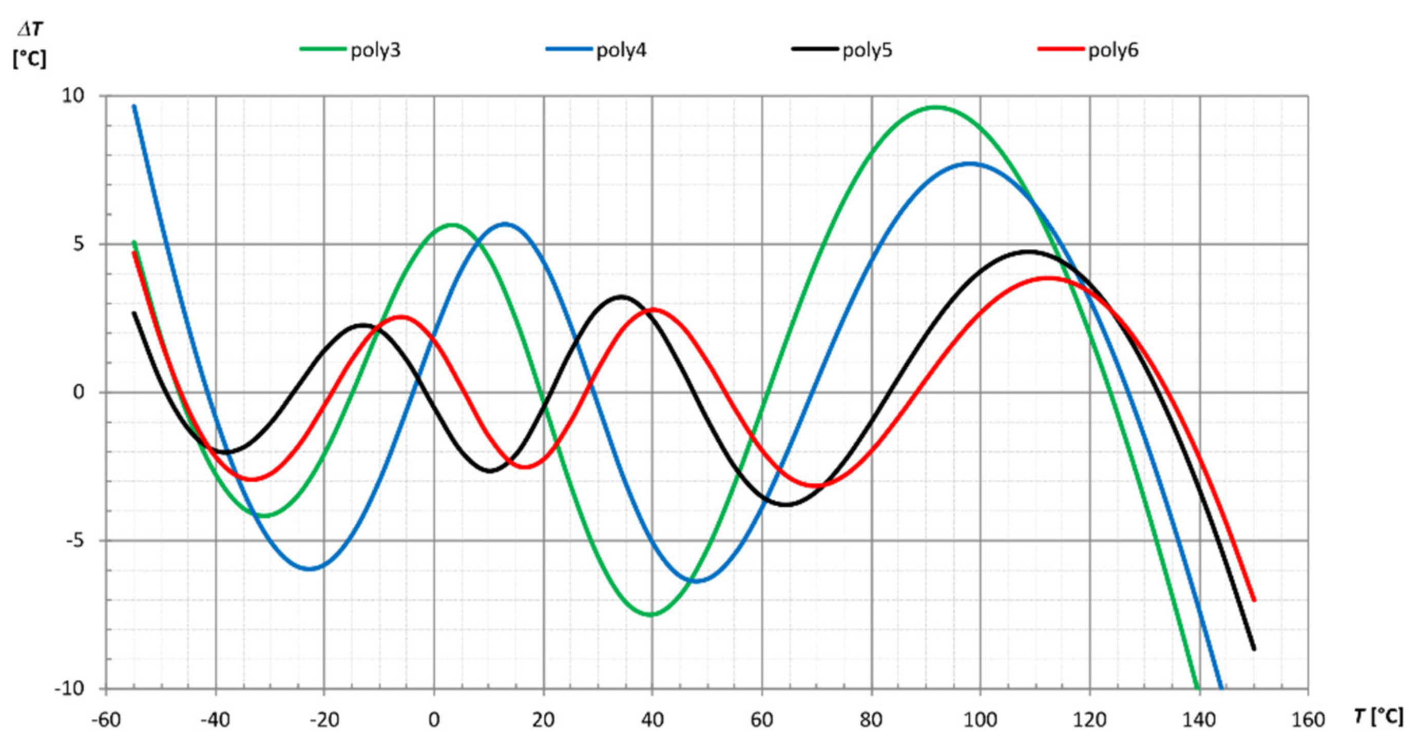
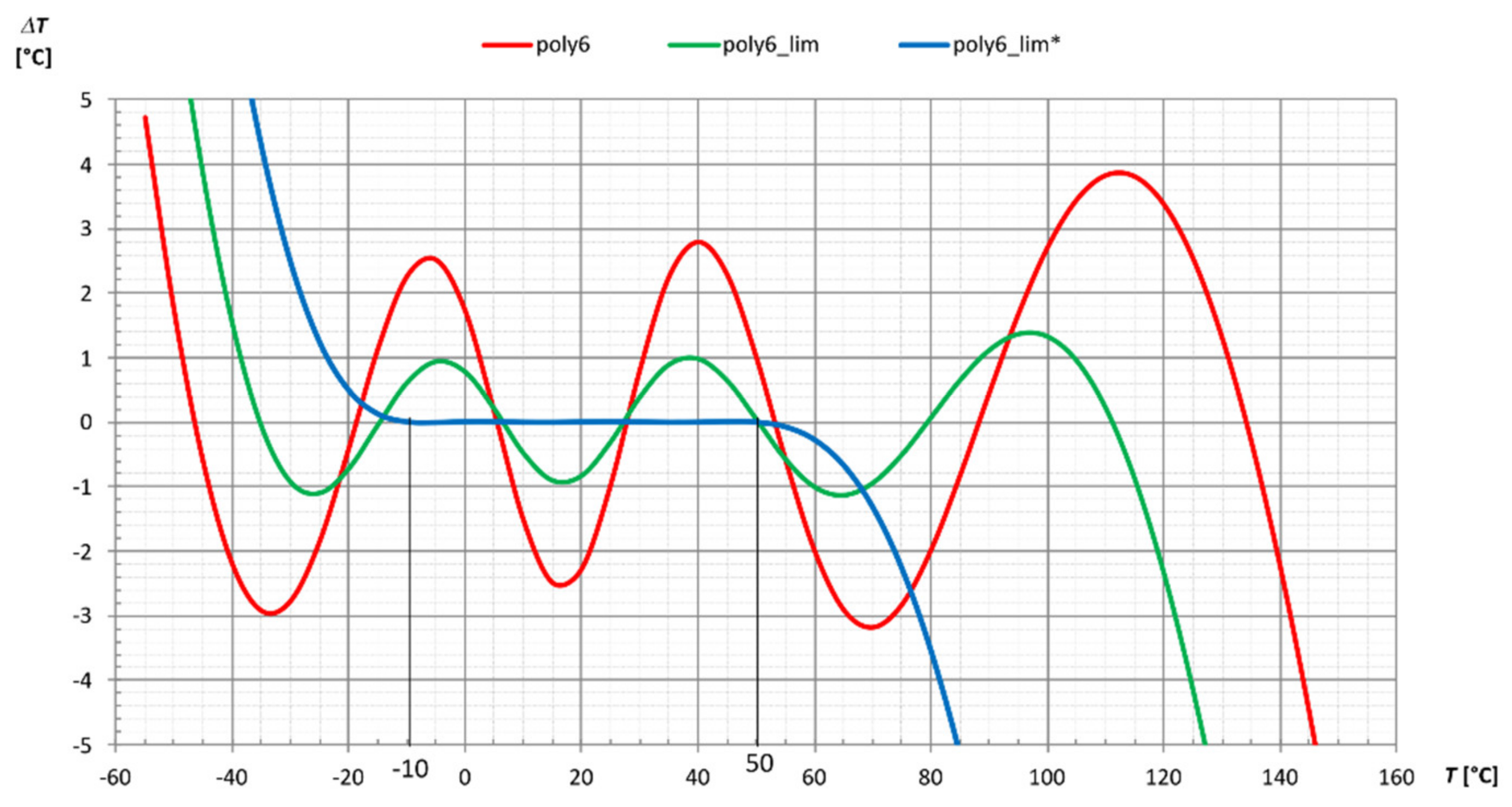
3.2. Approximation of Tabular Data with Polynomials

Similarly to the look-up method, the following approach relies on input data R(T) presented in table form. The third and fourth columns are extracted from the look-up table (Figure 5) to establish the correlation between T and U_T at given discrete points. Finally, a polynomial function T(U_T) is then fitted on these points in the preferred temperature range (Figure 8). A linear approximation can be acceptable if the temperature is to be measured on a smaller range than the nominal. This situation is depicted in Figure 8, where a trendline

$$T_{linear}=29.89·U_T-23.80.$$

(12)

is fitted for a limited temperature range from −10 °C to 50 °C. A closer look at the approximated curve reveals that the temperature error between the manufacturer data-based T(U_T) and the approximated (calculated) temperature T_linear(U_T) (labelled ΔT in Figure 9) is around ±1 °C.

If a wider temperature range is required, a higher-order approximation should be used to maintain the error within the initially set limit, resulting in a more complex and consequently more time-demanding (for the microcontroller) calculation procedure. As expected, the obtained results are more promising than the linear approximation can offer, as shown in Figure 10, where the temperature error is calculated for polynomials of the third, fourth, fifth and sixth order. For the latter, the analytical expression follows the syntax

$$\begin{gathered} T_{poly6}=a_6·u^6+a_5·u^5+a_4·u^4+a_3·u^3+ \\ +a_2·u^2+a_1·u+a_0, \end{gathered}$$

(13)

where a_i are the polynomial coefficients and u is the voltage U_T from the conditioning circuit. In all cases shown in Figure 10, the polynomial fitting was completed for the nominal temperature range (−55 °C to 150 °C). It is obvious that higher polynomial orders reduce the temperature error, yet not to such an extent as desired—especially if we compare it with the ±1 °C error obtained already by the first-order approximation—yet the latter was fitted to a narrower temperature range (Figure 9). Applying this approach, the error in Figure 10 can be further reduced if temperature measurement is confined to a narrower range. This is evident in Figure 11, where temperature error based on the sixth-order approximation is given, for three temperature ranges—the nominal (poly6) as already presented in Figure 10, then for a limited range from −40 °C to 120 °C (poly6_lim) and another one for a range from −10 °C to 50 °C (poly6_lim*). As seen, the lattermost temperature error is practically negligible, whereas the second shows a significant decrease compared to the first, i.e., to the polynomial fitted for the nominal range.

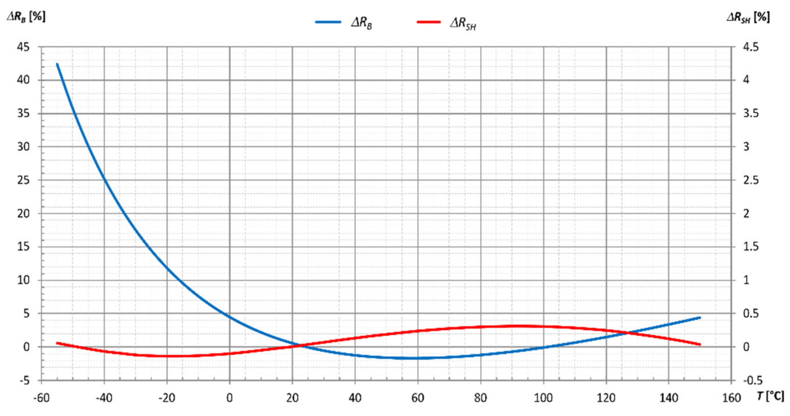
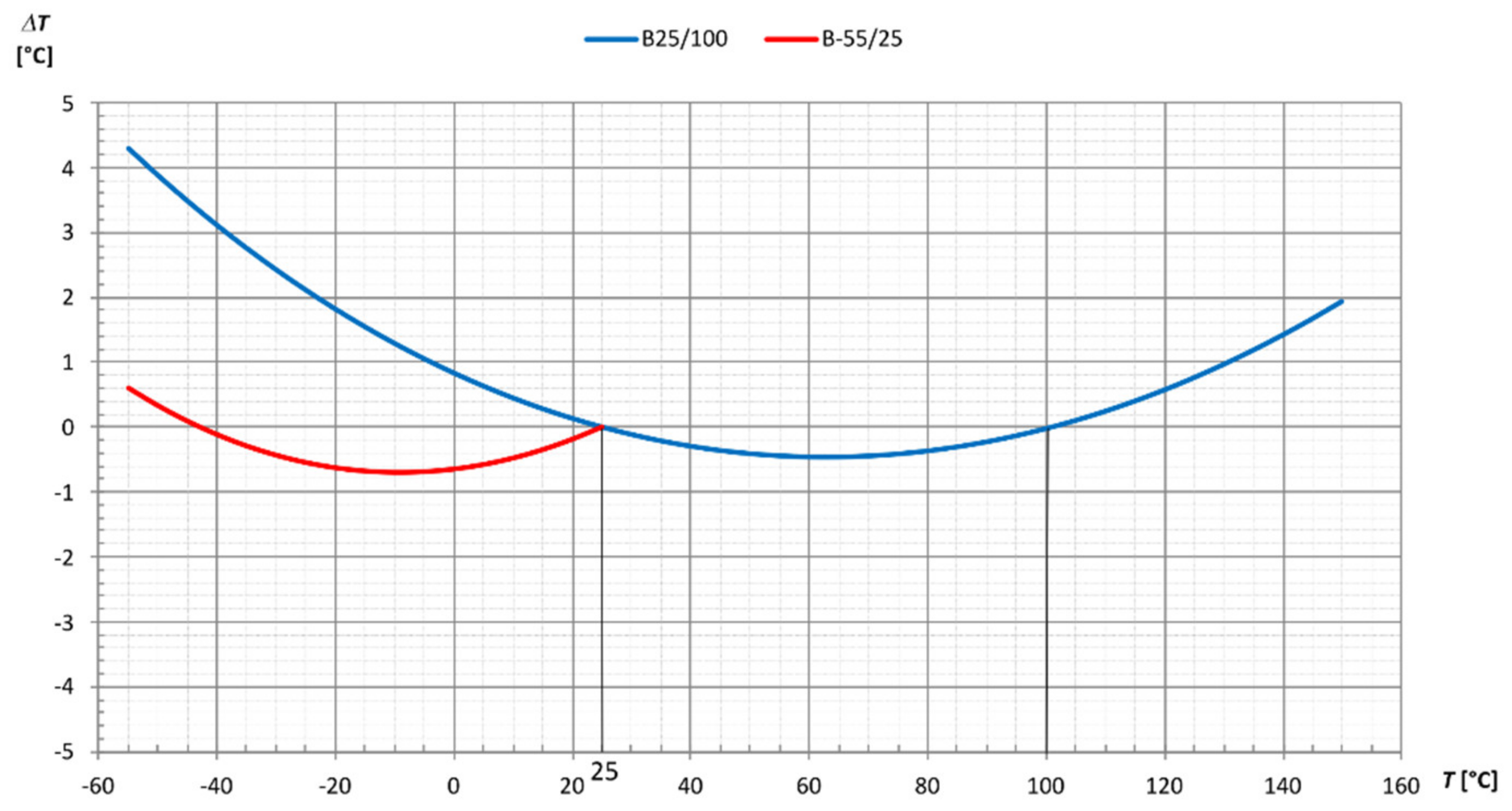
3.3. Analytical Approach Using the B Equation

In contrast to tabular-based methods, the following one is more straightforward as the analytical expression (5) is known at the procedure’s beginning—with its inherent limitations considered in Section 2. Their impacts reflect consequentially in measured voltage, obtained by inserting (5) into (8):

$$U_{T,meas}=U_{S+}·\frac{R_S}{R_0·e^{B\left(\frac{1}{T}-\frac{1}{T_0}\right)}+R_S}.$$

(14)

After antilog of (14) and rearrangement, the expression for temperature (in Kelvin) follows

$$T_{meas}=\frac{1}{\frac{1}{T_0}+\frac{1}{B}·\ln \left(\frac{R_S}{R_0}\left(\frac{U_{S+}}{U_{T,meas}}-1\right)\right)}.$$

(15)

The calculated temperature error is given in Figure 12. As expected, the temperature error is relatively small in the temperature range between 25 °C and 100 °C, where the implemented B_25/100 = 4000 K optimally describes the NTC thermistor.

If a wider temperature range should be covered, a suitable B, optimised for a low-temperature range, should be combined with the first one. As seen in Figure 12, an additional curve with B_−55/25 = 3750 K is included to significantly reduce the temperature error in the range from −55 °C to 25 °C. For a practical implementation, we should stress that the intersection point of both curves lies at 25 °C, where, due to the originally selected R_S = 10 kΩ and according to relation (8), the measured voltage should be U_T,meas = 1.65 V. Therefore, the calculation of temperature should be performed using B_25/100 for measured voltages U_T,meas ≥ 1.65 V, whereas for U_T,meas ≤ 1.65 V, we should use B_−55/25. Nevertheless, in practice, due to a possible discrepancy between nominal and actual B values, a calibration procedure as in [32] should be performed first in order to achieve the best results.

3.4. Analytical Approach Using the Steinhart–Hart Equation

In this case, we rely on the Steinhart–Hart Equation (1) to calculate the temperature T. Besides the Steinhart–Hart parameters (a, b and c), we need to know the resistance R of the thermistor. The procedure for resistance calculation using (2–4) has already been discussed. However, we have another option for practical implementation. Since the temperature is calculated indirectly utilising the voltage measurement, we can use the relation (8) at a given temperature:

$$R_{NTC}=R_S·\left(\frac{U_{S+}}{U_{T,meas}}-1\right).$$

(16)

After inserting (16) into the original Steinhart–Hart notation (1), we obtain the temperature (in Kelvin):

$$T_{meas}=\frac{1}{a+b·\ln \left(R_S·\left(\frac{U_{S+}}{U_{T,meas}}-1\right)\right)+c·{\left(\ln \left(R_S·\left(\frac{U_{S+}}{U_{T,meas}}-1\right)\right)\right)}^3}.$$

(17)

It can be seen that relation (15), which is used for the calculation of temperature with the B equation approach, is merely a simplification of (17) if the cubic part is neglected (c = 0) and a and b are calculated from relation (6). For practical implementation in the microcontroller, the procedure for temperature calculation following (17) is not overly complex, after all, provided that the Steinhart–Hart parameters are known. The benefit of using this approach is evident from Figure 13, where the temperature error is plotted for the whole temperature range using the thermistor manufacturer’s data from [28] and Steinhart–Hart parameters a = 1.139357363 × 10⁻³, b = 2.327048139 × 10⁻⁴ and c = 9.134393411 × 10⁻⁸ again.

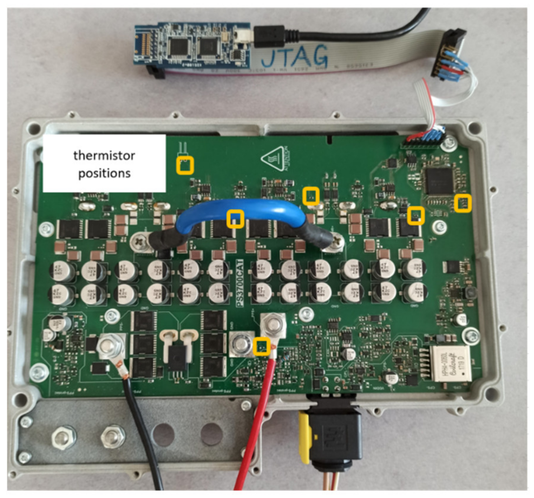
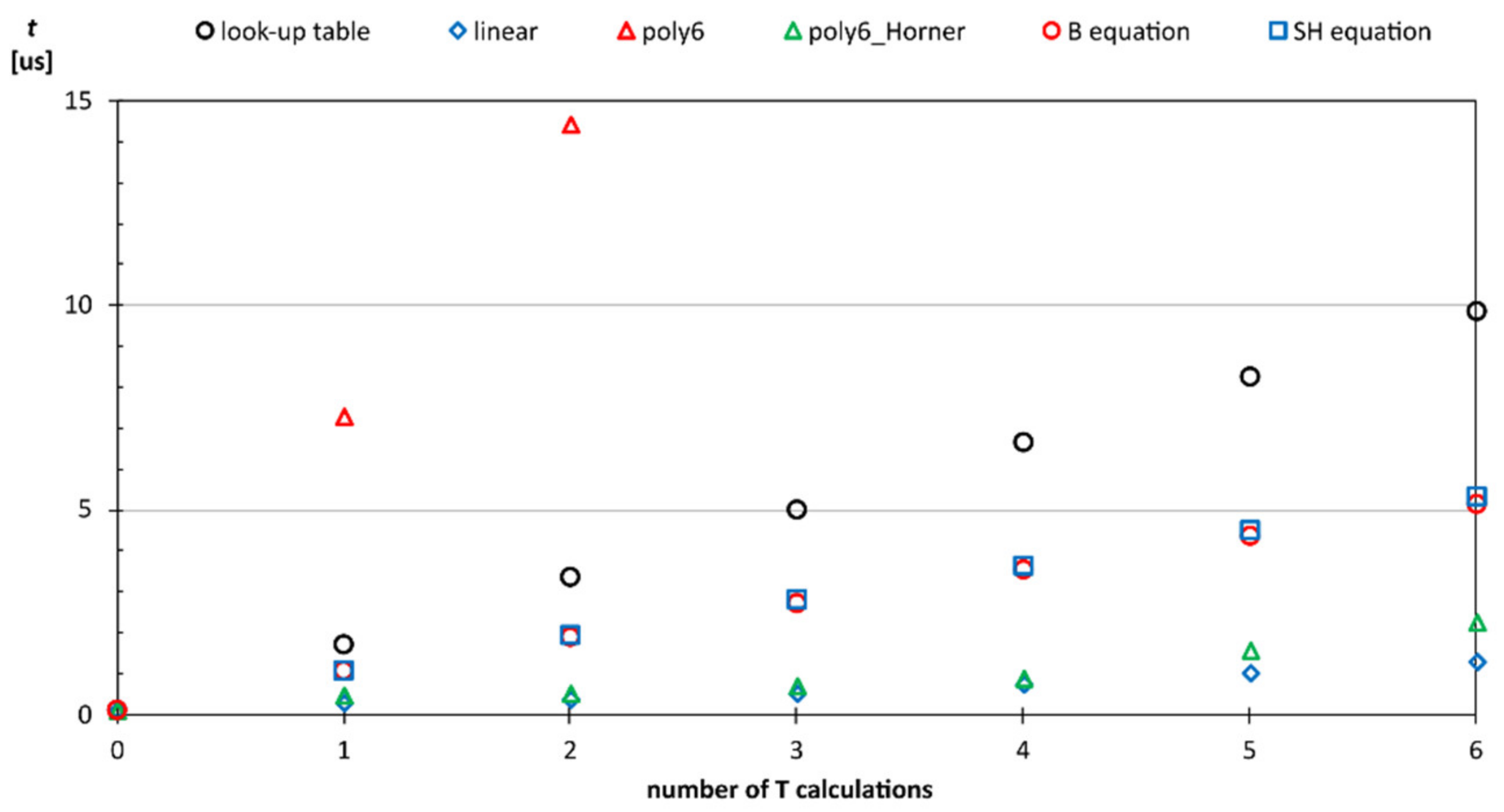
4. Experimental Results—Comparison of Methods

In the following section, all four presented methods for temperature calculation will be analysed in terms of the required prework and overall complexity, with a special focus on the execution time of the algorithm that runs in the microcontroller. We opted to calculate the temperature for up to six NTC thermistors for each approach in order to determine their influence on the calculation time needed for the MCU to execute the algorithm. A set of measurements was performed on a laboratory prototype of an advanced 3.7 kW DC/DC converter (Figure 14), designed for the automotive industry. Its topology is not essential for this paper, though further information can be found in [37]. In Figure 14, thermistor positions are marked in orange; some thermistors are located on the lower side of the printed circuit board (PCB).

The converter prototype is controlled by means of the Texas Instruments’ MCU TMS320F280049 [38] with a control algorithm executed at a frequency of 30 kHz, so the voltage at the ADC inputs is sampled every 33.3 µs. It must be stressed here that temperature calculations generally do not require such a high frequency. However, if the temperature is used for online diagnostics in safety-critical applications, then high bandwidth is mandatory. In our case, high sampling frequency is dictated by hardware and software. The primary function of the converter required precise sampling of currents at 30 kHz. As analog-to-digital converters (ADC) could not be configured to sample the temperature at a lower frequency while maintaining precise sampling of currents, the temperature was also sampled at the same frequency. Furthermore, to keep the software architecture unified and simple, temperature calculations were executed with the same frequency as the in calculation of other measured signals.

Obviously, adding rather complex calculation routines into the control algorithm of the electronic device is in contradiction with the tendency to use higher sampling frequencies for better accuracy of the primary control quantity in focus, since added routines increase the algorithm execution time.

In our test environment (Figure 14), temperature calculation algorithms were tested in the converter’s standby mode to avoid a possible severe malfunction if the algorithm execution time exceeds the pre-set time interrupt value of 33.3 μs. In the following, the required prework is first outlined for each presented calculation method, and then results for temperature calculation time are given.

• Look-Up Table

The investigated thermistor was supported with the manufacturer’s data for 5 °C intervals [28], but there are also data available for 1 °C intervals in [36], resulting in a larger MCU memory space requirement, yet yielding higher accuracy. In our case, an array of 42 values from [28]; curve no. 8502 for temperature and for calculated voltages U_T from the signal conditioning circuit using (8) was firstly prepared for the MCU used [38]. Then, at every time interrupt, the voltage U_T,meas at analog input was sampled and fed to the temperature calculation routine, which started with a search for two corresponding indexes (9) using a binary search method. Finally, the temperature was calculated using (11).

Starting from the standby mode of the converter and adding consecutive temperature calculations for six NTC thermistors installed on the PCB, the temperature calculation time in total was 9.87 μs. On average, each temperature calculation using the look-up table and a linear interpolation required 1.65 μs.

• Approximation of a Tabular Data with Polynomials

To test the polynomial approach, we chose to use a first-order and sixth-order polynomial for approximation of the temperature vs. voltage curve (as depicted in Figure 8). Firstly, the first-order polynomial (line) was examined, with a line fitted for a limited temperature range from −10 °C to 50 °C. Since the temperature was calculated using a simple notation (12), the expected calculation time for all six temperatures was relatively small. Nonetheless, the total time was 1.31 μs. On average, each temperature calculation using a linear approximation added 0.22 μs to the algorithm execution time.

Next, we tested two sixth-order polynomial notations, i.e., the original notation as written in (13) and a modified one using a Horner’s method notation to reduce the number of arithmetic operations:

$$T_{poly6}=\left(\left((((a_6·u+a_5\right)·u+a_4\right)·u+a_3)·u+a_2)·u+a_1)·u+a_0.$$

(18)

In both cases, the following polynomial parameters (rounded to four significant digits of precision) were used:

• a₆ = 3.7883;
• a₅ = −27.1741;
• a₄ = 59.5590;
• a₃ = −10.7668;
• a₂ = −109.7692;
• a₁ = 145.9399 and
• a₀ = −55.1190.

Polynomial parameters were calculated in advance based on calculated values of voltage (8) and thermistor data using the LINEST function in Excel for the nominal temperature range (−55 °C to 150 °C; labelled poly6).

As expected, there was a significant difference in the algorithm execution time between polynomial notations (13) and (18). With the first one, with only one temperature, the calculation time was already 7.29 μs. With two temperature calculation routines, the calculation time increased to 14.42 μs, so further temperatures were not tested since the maximum available time limit for temperature calculations was reached. Namely, the control algorithm for the converter itself needed around 18 μs. With the Horner notation (18), calculation times were significantly lower. Namely, the calculation time for all six temperatures was 2.28 μs (on average, each NTC temperature measurement required 0.38 μs), which speaks in favour of Horner’s polynomial notation.

• Analytical Method Using the B Equation

This method requires less prework since the measured voltage U_T is fed directly to the temperature calculation routine based on (15), which only needs some predefined constants that are related to the thermistor and the signal conditioning circuit. During the experiment, only results for the initially presented method with a B_25/100 constant (Figure 12) were monitored, yielding a total calculation time of 5.16 μs (on average, 0.86 μs per one NTC temperature channel).

• Analytical Method Using the Steinhart–Hart Equation

With this approach, we also start with the measured voltage U_T that is (directly or through “extraction” of resistance R_NTC using (16)) fed to the temperature calculation routine (17). For the latter, however, the Steinhart–Hart parameters need to be defined in advance. In our case, the manufacturer did not provide them, so we used an online tool [31] together with the manufacturer resistance data at three temperatures, so they were not a result of a calibration procedure, as in [39]. As suggested in [30], we used two temperatures that coincided with the nominal temperature range, i.e., −55 °C and 150 °C and a point between them—we opted for 25 °C—thus resulting in a = 1.139357363 × 10⁻³, b = 2.327048139 × 10⁻⁴ and c = 9.134393411 × 10⁻⁸. It must be stressed here that, in terms of the required calculation time, notation (17) is not overly complex compared to (15), since, in both cases, a natural algorithm (ln) operation is performed first, followed by one or more multiplications. For a selected set of values, all six temperature calculations resulted in the calculation time of 5.32 μs (on average, each NTC temperature measurement required 0.89 μs), which is comparable to results calculated with the B equation.

Obtained results of the MCU load for all four calculation methods are summarised in Figure 15. It is clear that the look-up table method with linear interpolation (11) results in high calculation times, although there are no complex arithmetic operations involved. However, the significant time increase is related to a time-demanding binary search algorithm of appropriate indexes from the look-up table, for which the microcontroller is not optimised. With the polynomial approximation method, the first-order linear approximation (12) is, in terms of calculation time, quite comparable to the sixth-order Horner notation (18) (labelled poly6_Horner). In contrast, the original polynomial notation (13) (poly6) requires by far the most time. As suspected, both the B equation and the Steinhart–Hart equation require similar MCU resources, though more than double that required for the polynomial methods. However, in regard to Figure 2, Figure 12 and Figure 13, the results are clearly more in favour of the Steinhart–Hart equation. In general, it does require more computational power than polynomial methods. However, it performs excellently—almost comparably to the look-up table—on the whole nominal temperature range, which is not the case for either the polynomial approximation or the B equation.

5. Discussion

The design process of complex electronic devices always requires many compromises that relate to various areas. In the presented paper, we focused on challenges associated with temperature measurement in a complex electronic device using a simple conditioning circuit with an NTC thermistor.

The main objective of the paper was to identify the influence of different temperature calculation routines on the MCU calculation time. Additionally, the intention was to select a method that can result in an acceptable temperature error (maximum ±1 °C) in the broadest—preferably nominal—temperature range of the thermistor. The signal conditioning circuit was assumed to be ideal, so the temperature error was introduced solely by the method itself.

Table 1. Comparison of key parameters of calculation methods.

	Look-Up Table with Interpolation	Polynomial Approximation		B Equation	Steinhart–Hart Equation
Parameter Observed		1st Order	6th Order
required prework	−/o	o	−/o	o/+	o/+
accuracy (limited range)	+	+	+	+	+
accuracy (nominal range)	+	−	−/o	o	+
MCU load	−	+	+	o	o

gives an overview of crucial parameters observed during the simulation and experimental tests. The sign “+” speaks in favour of the method, the sign “–” advises against the use of the method and the sign “o” indicates neutrality in this respect.

After all four presented methods were analysed and tested, we could conclude that the selection in fact depends on the available MCU resources. Namely, the temperature calculation using the look-up table or the Steinhart–Hart equation is far superior to other methods in terms of accuracy. On the other hand, these methods use significantly more MCU resources compared to polynomial methods—the first one essentially because of a time demanding index search routine in the look-up table and the second due to the calculation of the natural logarithm function. It is true, though, that temperature calculations could be performed with a lower sampling frequency compared to the sampling frequency of currents and voltages; however, this disrupts the otherwise unified algorithm structure, with only one time interrupt request. However, in the case of a possible MCU overload, we could implement a sequential routine with only one temperature calculation per interrupt cycle. Thus, we could summarise that the look-up table and the Steinhart–Hart method are the top choices when searching for an algorithm that offers a reasonably small error in the whole temperature range. If a narrower temperature range is tolerated, surprisingly good results in terms of accuracy and, above all, in terms of calculation time can be obtained with the higher-order polynomial method. Nonetheless, if a high accuracy of temperature measurement is of interest instead of the MCU load, then the look-up table would certainly be preferable.

References

1. Jaraczewski, M.; Mielnik, R.; Gębarowski, T.; Sułowicz, M. Low-Frequency Signal Sampling Method Implemented in a PLC Controller Dedicated to Applications in the Monitoring of Selected Electrical Devices. Electronics 2021, 10, 442. [Google Scholar] [CrossRef]
2. Gleissner, M.; Bakran, M.M. Design and Control of Fault-Tolerant Nonisolated Multiphase Multilevel DC–DC Converters for Automotive Power Systems. IEEE Trans. Ind. Appl. 2016, 52, 1785–1795. [Google Scholar] [CrossRef]
3. Siouane, S.; Jovanović, S.; Poure, P. Open-Switch Fault-Tolerant Operation of a Two-Stage Buck/Buck–Boost Converter with Redundant Synchronous Switch for PV Systems. IEEE Trans. Ind. Electron. 2019, 66, 3938–3947. [Google Scholar] [CrossRef]
4. Xu, L.; Ma, R.; Xie, R.; Xu, J.; Huangfu, Y.; Gao, F. Open-Circuit Switch Fault Diagnosis and Fault-Tolerant Control for Output-Series Interleaved Boost DC-DC Converter. IEEE Trans. Transp. Electrif. 2021. [Google Scholar] [CrossRef]
5. Zhu, Y.; Li, J.; Zhang, C.; Wang, W.; Wang, H. High Temperature Dry Tribological Behavior of Nb-Microalloyed Bearing Steel 100Cr6. Materials 2021, 14, 5216. [Google Scholar] [CrossRef]
6. Billard, M.W.; Basantani, H.A.; Horn, M.W.; Gluckman, B.J. A Flexible Vanadium Oxide Thermistor Array for Localized Temperature Field Measurements in Brain. IEEE Sens. J. 2016, 16, 2211–2212. [Google Scholar] [CrossRef]
7. Haberl-Meglič, S.; Levičnik, E.; Luengo, E.; Raso, J.; Miklavčič, D. The effect of temperature and bacterial growth phase on protein extraction by means of electroporation. Bioelectrochemistry 2016, 112, 77–82. [Google Scholar] [CrossRef]
8. Grigorov, E.; Kirov, B.; Marinov, M.B.; Galabov, V. Review of Microfluidic Methods for Cellular Lysis. Micromachines 2021, 12, 498. [Google Scholar] [CrossRef]
9. Gagliano, S.; Cairone, F.; Amenta, A.; Bucolo, M. A Real Time Feed Forward Control of Slug Flow in Microchannels. Energies 2019, 12, 2556. [Google Scholar] [CrossRef] [Green Version]
10. Shi, B.; Feng, S.; Shi, L.; Shi, D.; Zhang, Y.; Zhu, H. Junction Temperature Measurement Method for Power mosfets Using Turn-On Delay of Impulse Signal. IEEE Trans. Power Electron. 2018, 33, 5274–5282. [Google Scholar] [CrossRef]
11. Stella, F.; Pellegrino, G.; Armando, E.; Daprà, D. Online Junction Temperature Estimation of SiC Power MOSFETs through On-State Voltage Mapping. IEEE Trans. Ind. Appl. 2018, 54, 3453–3462. [Google Scholar] [CrossRef]
12. Matei, C.; Urbonas, J.; Votsi, H.; Kendig, D.; Aaen, P.H. Dynamic Temperature Measurements of a GaN DC–DC Boost Converter at MHz Frequencies. IEEE Trans. Power Electron. 2020, 35, 8303–8310. [Google Scholar] [CrossRef]
13. Bajzek, T.J. Thermocouples: A sensor for measuring temperature. IEEE Instrum. Meas. Mag. 2005, 8, 35–40. [Google Scholar] [CrossRef]
14. Burta, A.; Szabo, R.; Gontean, A. Temperature Measurements with Thermocouples Used in a Thermo-electric Hybrid Solar System. In Proceedings of the 2020 Fourth World Conference on Smart Trends in Systems, Security and Sustainability (WorldS4), London, UK, 27–28 July 2020; pp. 614–619. [Google Scholar] [CrossRef]
15. Muchenedi, H.K.; Prabu, P.S.; Madhu Mohan, M. Fabrication of Ferroelectric Liquid Crystal Thermistor. IEEE Trans. Electron Devices 2020, 67, 5063–5068. [Google Scholar] [CrossRef]
16. Texas Instruments. TMP23x Low-Power, High-Accuracy Analog Output Temperature Sensors. Available online: https://www.ti.com/lit/ds/symlink/tmp235.pdf (accessed on 19 August 2021).
17. Aleksic, S.O.; Mitrovic, N.S.; Lukovic, M.D.; Veljovic-Jovanovic, S.D.; Lukovic, S.G.; Nikolic, M.V.; Aleksic, O.S. A Ground Temperature Profile Sensor Based on NTC Thick Film Segmented Thermistors: Main Properties and Applications. IEEE Sens. J. 2018, 18, 4414–4421. [Google Scholar] [CrossRef]
18. Deng, X.; Cheng, Y.; Li, L.; Feng, J.; Cui, L.; Du, C.; Zhang, L.; Zhang, L.; Qin, J. Design and Application of High-Precision Temperature Measuring Instrument for Ice Cover Profile of River Based on the Resistance Residual Compensation Method. IEEE Access 2020, 8, 7899–7906. [Google Scholar] [CrossRef]
19. Sun, J.; Wu, K.; Fan, M.; Meng, F.; Cai, M.; Zhao, T.; Yang, C.; Xing, H.; Ye, W. Thermistor-Based Nematic Liquid Crystal IM95100-000. IEEE Trans. Electron Devices 2021, 68, 4064–4069. [Google Scholar] [CrossRef]
20. Kumar, V.N.; Narayana, K.V.L.; Bhujangarao, A.; Sankar, S. Development of an ANN-Based Linearization Technique for the VCO Thermistor Circuit. IEEE Sens. J. 2015, 15, 886–894. [Google Scholar] [CrossRef]
21. Wang, C.; Hou, Z.; You, J. Temperature-to-Frequency Converter With 1.47% Error Using Thermistor Linearity Calibration. IEEE Sens. J. 2019, 19, 4804–4811. [Google Scholar] [CrossRef]
22. Rana, K.P.S.; Kumar, V.; Dagar, A.K.; Chandel, A.; Kataria, A. FPGA Implementation of Steinhart–Hart Equation for Accurate Thermistor Linearization. IEEE Sens. J. 2018, 18, 2260–2267. [Google Scholar] [CrossRef]
23. Bandyopadhyay, S.; Das, A.; Mukherjee, A.; Dey, D.; Bhattacharyya, B.; Munshi, S. A Linearization Scheme for Thermistor-Based Sensing in Biomedical Studies. IEEE Sens. J. 2016, 16, 603–609. [Google Scholar] [CrossRef]
24. Sarkar, A.R.; Dey, D.; Munshi, S. Linearization of NTC Thermistor Characteristic Using Op-Amp Based Inverting Amplifier. IEEE Sens. J. 2013, 13, 4621–4626. [Google Scholar] [CrossRef]
25. Nenova, Z.P.; Nenov, T.G. Linearization Circuit of the Thermistor Connection. IEEE Trans. Instrum. Meas. 2009, 58, 441–449. [Google Scholar] [CrossRef]
26. Chatterjee, N.; Bhattacharyya, B.; Dey, D.; Munshi, S. A Combination of Astable Multivibrator and Microcontroller for Thermistor-Based Temperature Measurement over Internet. IEEE Sens. J. 2019, 19, 3252–3259. [Google Scholar] [CrossRef]
27. Venkata, K.; Narayana, L.; Kumar, V.N. Development of an Intelligent Temperature Transducer. IEEE Sens. J. 2016, 16, 4696–4703. [Google Scholar] [CrossRef]
28. TDK. NTC Thermistors for Temperature Measurement. Available online: https://product.tdk.com/system/files/dam/doc/product/sensor/ntc/chip-ntc-thermistor/data_sheet/50/db/ntc/ntc_smd_automotive_series_0603.pdf (accessed on 19 August 2021).
29. Steinhart, J.S.; Hart, S.R. Calibration curves for thermistors. Deep Sea Res. Oceanogr. Abstr. 1968, 15, 497–503. [Google Scholar] [CrossRef]
30. Stanford Research Systems. Calibrate Steinhart-Hart Coefficients for Thermistors. Application Note. Available online: https://www.thinksrs.com/downloads/PDFs/ApplicationNotes/LDC%20Note%204%20NTC%20Calculator.pdf (accessed on 19 August 2021).
31. Stanford Research Systems. Thermistor Calculator. Available online: https://www.thinksrs.com/downloads/programs/therm%20calc/ntccalibrator/ntccalculator.html (accessed on 19 August 2021).
32. Liu, Y.; Liu, Y.; Zhang, W.; Zhang, J. The Study of Temperature Calibration Method for NTC Thermistor. In Proceedings of the 4th International Conference on Frontiers of Sensors Technologies (ICFST), Shanghai, China, 6–9 November 2020; pp. 50–53. [Google Scholar] [CrossRef]
33. Vaegae, N.K.; Narayana, K.V.L. Development of thermistor signal conditioning circuit using artificial neural networks. IET Sci. Meas. Technol. 2015, 9, 955–961. [Google Scholar] [CrossRef]
34. Mahaseth, D.N.; Kumar, L.; Islam, T. An efficient signal conditioning circuit to piecewise linearizing the response characteristic of highly nonlinear sensors. Sens. Actuators A: Phys. 2018, 280, 559–572. [Google Scholar] [CrossRef]
35. Jovanović, J.; Denić, D. NTC Thermistor Nonlinearity Compensation Using Wheatstone Bridge and Novel Dual-Stage Single-Flash Piecewise-Linear ADC. Metrol. Meas. Syst. 2021, 28, 523–537. [Google Scholar] [CrossRef]
36. TDK. NTC B57351V5103H060 RT Sheet. Available online: https://product.tdk.com/system/files/dam/doc/product/sensor/ntc/chip-ntc-thermistor/rt_sheets/b57351v5103h060.csv (accessed on 19 August 2021).
37. Petkovsek, M.; Zajec, P. Evaluating Common-Mode Voltage Based Trade-Offs in Differential-Ended and Single-Supplied Signal Conditioning Amplifiers. Electronics 2021, 10, 1982. [Google Scholar] [CrossRef]
38. Texas Instruments. TMS320F280049 Microcontroller. Available online: https://www.ti.com/product/TMS320F280049 (accessed on 19 August 2021).
39. Chen, C. Evaluation of resistance–temperature calibration equations for NTC thermistors. Measurement 2009, 42, 1103–1111. [Google Scholar] [CrossRef]
Figure 1. Calculated and measured resistance of 10 kohm NTC thermistor (logarithmic scale).
Mathematics 09 02266 g001
Figure 2. Resistance error for B equation and Steinhart–Hart equation.
Mathematics 09 02266 g002
Figure 3. Conditioning circuit: (a) Proposed; (b) Optional.
Mathematics 09 02266 g003
Figure 4. Influence of resistance RS value: (a) Voltage vs. temperature; (b) Voltage measurement sensitivity vs. temperature.
Mathematics 09 02266 g004
Figure 5. Look-up table principle.
Mathematics 09 02266 g005
Figure 7. Temperature error with look-up table and linear interpolation.
Mathematics 09 02266 g007
Figure 8. Temperature vs. calculated voltage for manufacturer-based data and linear approximation.
Mathematics 09 02266 g008
Figure 9. Temperature error for linear approximation.
Mathematics 09 02266 g009
Figure 10. Temperature error for different polynomial order approximations—fitted across nominal temperature range.
Mathematics 09 02266 g010
Figure 11. Temperature error for 6th-order polynomial approximation—fitted across different temperature ranges: nominal and limited (poly6_lim, poly6_lim*).
Mathematics 09 02266 g011
Figure 12. Temperature error for combined B equation-based expression.
Mathematics 09 02266 g012
Figure 13. Temperature error for Steinhart–Hart equation-based expression.
Mathematics 09 02266 g013
Figure 14. Experimental set-up.
Mathematics 09 02266 g014
Figure 15. Time comparison of different temperature calculation methods.
Mathematics 09 02266 g015