Improved Manta Ray Foraging Optimization for Parameters Identification of Magnetorheological Dampers

Abstract

Magnetorheological (MR) dampers play a crucial role in various engineering systems, and how to identify the control parameters of MR damper models without any prior knowledge has become a burning problem. In this study, to identify the control parameters of MR damper models more accurately, an improved manta ray foraging optimization (IMRFO) is proposed. The new algorithm designs a searching control factor according to a weak exploration ability of MRFO, which can effectively increase the global exploration of the algorithm. To prevent the premature convergence of the local optima, an adaptive weight coefficient based on the Levy flight is designed. Moreover, by introducing the Morlet wavelet mutation strategy to the algorithm, the mutation space is adaptively adjusted to enhance the ability of the algorithm to step out of stagnation and the convergence rate. The performance of the IMRFO is evaluated on two sets of benchmark functions and the results confirm the competitiveness of the proposed algorithm. Additionally, the IMRFO is applied in identifying the control parameters of MR dampers, the simulation results reveal the effectiveness and practicality of the IMRFO in the engineering applications.

1. Introduction

Magnetorheological (MR) dampers are a kind of intelligent semi-active control device, the output damping force of the damper can be controlled by controlling the current instruction in the coil [1,2]. MR dampers are famous for their fast reaction speed, less energy consumption and wide control range; therefore, MR dampers are widely applied in various engineering domains, e.g., vehicle systems [3,4]. However, the mathematical models of MR dampers are very complicated because of their special mechanical characteristic-hysteretic property. Xu et al. [5] introduced a new single-rod MR damper with combined volume compensator; meanwhile, the design method of the combined compensator with independent functions of volume compensation and compensation force was proposed. Yu et al. [6] proposed a novel compact rotary MR damper with variable damping and stiffness and a unique structure that contains two driven disks and an active rotary disk was designed. Boreiry et al. [7] investigated the chaotic response of a nonlinear seven-degree-of-freedom full vehicle model equipped with an MR damper, and the equations of motion was proposed by employing the modified Bouc–Wen model for an MR damper. Many MR dampers have emerged with different uses and functions. Among them, the Bouc–Wen model is a typical one, which contains numerous unknown parameters. In addition, a range of other factors, including the current size, piston speed and excitation factors, also affect the accuracy of the model, which makes parameter identification of the model more difficult. Therefore, how to find an effective method to identify the control parameters of MR dampers is of great importance and has become a challenging task. In addition, the possible magneto-thermal problem of the MR damper to MR fluid is also becoming a pressing issue [8,9,10].

With the rapid development of computer technologies, meta-heuristic algorithms, a suitable technology, are applied in MR dampers to establish a set of accurate and reliable models. Many scholars at home and abroad carry out the relevant research work and have achieved some results. Giuclea et al. [11] used a genetic algorithm (GA) to identify the control parameters of a modified Bouc–Wen model, in which the applied currents are determined using the curve fitting method. However, in addition to the implementation complexity, a GA may suffer from premature convergence and its optimization performance depends mostly on the probability election for crossover, mutation and selecting operators [12]. Kwok et al. [13] gave a parameter identification technique for a Bouc–Wen damper model using particle swarm optimization (PSO), and some experimental force–velocity data under various operating conditions were employed. Although PSO is improved by using a stop criterion in this study, it easily traps into the local optima and suffers from premature convergence [14]. Thus, the application of PSO in MR dampers is limited, owing to its drawbacks of nature.

Despite the shortcomings of PSO and GAs, meta-heuristic methods are particularly popular for their randomness, easy implementation and black box treatment of problems [15,16]. An increasing number of scholars have proposed meta-heuristic algorithms inspired from different mechanisms by studying animal behaviors and physical phenomena in nature [17,18,19]. Some of the most popular algorithms are the bat algorithm (BA) [20], squirrel search algorithm (SSA) [21], artificial ecosystem-based optimization [22], whale optimization algorithm (WOA) [23], virus colony search (VCS) [24], fruit fly optimization algorithm (FOA) [25], butterfly optimization algorithm (BOA) [26], spotted hyena optimizer (SHO) [27], grasshopper optimization algorithm (GOA) [28], flower pollination algorithm (FPA) [29], crow search algorithm (CSA) [30], grey wolf optimizer (GWO) [31], water cycle algorithm (WCA) [32], gravitational search algorithm (GSA) [33], atom search optimization (ASO) [34], henry gas solubility optimization (HGSO) [35], charged system search (CSS) [36], water evaporation optimization (WEO) [37], equilibrium optimizer (EO) [38] and supply–demand-based optimization (SDO) [39]. In the last ten years, a great number of bio-inspired optimization and nature-inspired optimization algorithms have been proposed. These algorithms are significantly distinct in their natural or biological inspirations; therefore, one can find its category easily and without any ambiguity. In addition, the algorithms are different with respect to their search behaviors, i.e., how they update new candidate solutions during the iteration process [40]. Although these meta-heuristic methods perform well in tackling some challenging real-world problems, they have some disadvantages and their optimization performance still remains to be improved, especially for some inherently high-nonlinear and non-convex problems, such as the economic dispatch (ED) problem [41]. To overall the drawbacks of these algorithms, hybridization might produce new algorithmic behaviors that are effective in improving the optimization performance of the algorithms.

Manta ray foraging optimization (MRFO) [42,43] is a new meta-heuristic algorithm, which simulates the foraging behavior of manta rays in nature. The local exploitation is performed by the chain foraging and somersault foraging behaviors, while the global exploration is performed by the cyclone foraging behavior. This algorithm shows some optimization capabilities and is very successful in applying in some engineering domains, such as geophysics [44], energy allocation [45,46,47], image processing [48] and electric power [49]. These successful applications in the literature confirm MRFO is effective in solving different complex real-world problems. Even though MRFO belongs to a category of meta-heuristic algorithms, it is significantly distinct from other widely employed meta-heuristics in terms of ideology and conception. The major difference between MRFO and PSO is their different biology behaviors. PSO is inspired by the movement of bird flocks or fish schools in nature, whereas MRFO is inspired by the social foraging behaviors of manta rays. Another distinct difference between both is the solution searching mechanism. The solutions in PSO are produced by the combination of the global best solution found thus far and the local best solution, as well as the movement velocity of the individuals; whereas, in MRFO, the solutions are produced by the combination of the global best solution found thus far and the solution in front of it by switching different movement strategies. For a GA and MRFO, both are quite different. A GA is inspired by Darwin’s theory of evolution, which is quite different from the social foraging behaviors of manta rays in MRFO. The second difference is the representation of problem variables. In GAs, the problem variables are encoded in a series of fixed-length bit strings; in MRFO, the problem variables are used directly. Moreover, in GAs, by performing the roulette wheel selection strategy, better solutions have a greater probability of creating new solutions, and worse solutions are probably replaced by new better solutions [27]. While in MRFO, all the individuals in the population have the same probability of improving their solutions. Although both MRFO and bacterial foraging optimization (BFO) [50] are swarm-based and bio-inspired meta-heuristic techniques, which model the biology foraging behaviors, there are still some significant differences. The major difference between MRFO and BFO is that the concepts of searching in the foraging behaviors are different. MRFO models three foraging behaviors of manta rays including chain foraging, cyclone foraging and somersault foraging, while BFO models the social foraging behaviors of Escherichia coli, such as chemotaxis, swarming, reproduction and elimination–dispersal. The second difference is that BFO produces new solutions by adding a random direction with a fixed-length step pace, whereas MRFO produces new solutions with respect to the best solution and the solution in front of it. Additionally, in BFO, when updating the solutions, half of the solutions with higher health are reproduced and half of the solutions with lower health are discarded; MRFO accepts new solutions that are better than current solutions. The last difference between both is that BFO uses the health degree of the bacteria as the fitness values of solutions, while MRFO generally uses the function values of the given problems as the fitness values of solutions. It is obvious that BFO and MRFO follow totally different approaches when solving optimization problems.

However, similar to other meta-heuristics, MRFO also suffers from some disadvantages, i.e., premature convergence, trapping into the local optima and weak exploration [51,52]. There are many scholars who adopt various methods to enhance the performance of MRFO in the literature. Turgut [51] integrated the best performing ten chaotic maps into MRFO and proposed a novel chaotic MRFO to the thermal design problem, this improved version can effectively escape the local optima and increase the convergence rate of the algorithm. Calasan et al. [53] enhanced the optimization ability of the algorithm by integrating the chaotic numbers produced by the Logistic map in MRFO, this variant was used to estimate the transformer parameters. Houssein et al. [52] proposed an efficient MRFO algorithm by hybridizing opposition-based learning with initialization steps of MRFO, which was used to solve the image segmentation problem. Hassan et al. [54] solved the economic emission dispatch problems through hybridizing the gradient-based optimizer with MRFO, which may lead to the avoidance of local optima and accelerate the conveyance rate. Elaziz et al. [55] utilized the heredity and non-locality properties of the Grunwald–Letnikov fractional differ-integral operator to improve the exploitation ability of the algorithm. Elaziz et al. [56] proposed the modified MRFO based on differential evolution as an effective feature selection approach to identify COVID-19 patients by analyzing their chest images. Jena et al. [57] introduced a new attacking MRFO algorithm, which was used for the maximum 3D Tsallis entropy based multilevel thresholding of a brain MR image. Yang et al. [58] devised a hybrid Framework based on MRFO and grey prediction theory to forecast and evaluate the influence of PM10 on public health. Ramadan et al. [59] used MRFO to search for a feasible configuration of the distribution network to achieve fault-tolerance and fast recovery reliable configurable DN in smart grids. Houssein et al. [60] used MRFO to extract the PV parameters of single, double and triple-diode models. It shows better abilities to exploit the search space for unimodal problems, but the weak exploration and easily trapping into the local optima for multimodal problems as well as the unbalance between exploration and exploration for hybrid problems are still a few of the major issues.

It can be obvious that it is feasible to design some improved versions of MRFO, and the above implementations are good examples of this capability. However, it seems difficult for these improved versions to simultaneously improve their overall optimization capabilities combined with the shortcomings of the algorithm, such as exploration, exploitation, balance between both and convergence rate. Therefore, it is necessary to conduct some research attempts to establish a comprehensive improvement strategy for effectively tracking complex optimization problems. Based on the investigations mentioned above, a new hybrid model by combining different operators and designing some search strategies to comprehensively enhance the optimization performance of the algorithm is one of the major research attempts. This is the main motivation of this study. An effective optimization method can accurately obtain the parameters of the complex MR damper. These selected parameters have large influences on the output damping force, which gives the damper better hysteretic and dynamic characteristics. Therefore, it has a wide application value in industry and civil fields at home and abroad.

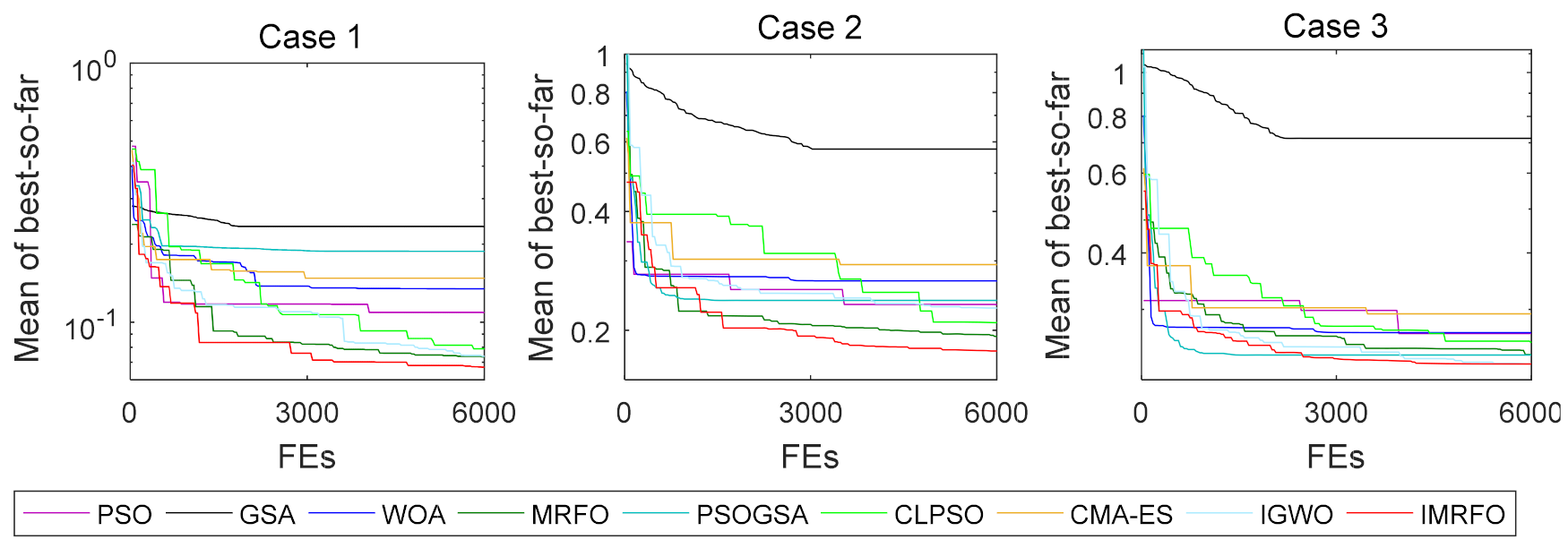
In light of the fact mentioned above, a hybrid MR damper model based on an optimization technique is proposed in this study. To obtain the optimal control parameters of the MR damper, an improved MRFO (IMRFO) combing a searching control factor, an adaptive weight coefficient with the Levy flight and a wavelet mutation are presented. Firstly, based on the analysis for the exploration probability of MRFO, the weak exploration capability of MRFO is promoted by introducing the searching control mechanism, in which a searching control factor is proposed to adaptively adjust the search option according to the number of iterations, promoting the exploration ability of the algorithm. Secondly, the weight coefficient in the cyclone foraging is redefined by combining with the Levy flight; this search mechanism can effectively promote the diversity of search individuals and prevent the premature convergence of local optima. Finally, the Morlet wavelet mutation strategy is employed to dynamically adjust the mutation space by calculating the energy concentration of the wavelet function; this strategy can improve the ability of the algorithm to step out of stagnation and the convergence rate. The effectiveness of the IMRFO is verified on two sets of standard benchmark functions. Additionally, the proposed IMRFO has been applied to optimally identify the control parameters of the MR dampers. The results have been compared with those of other algorithms, demonstrating the superiority of the IMRFO in solving the complex engineering problems.

The novelty points of this study are highlighted below.

In this study, a searching control factor, an adaptive weight coefficient and a wavelet mutation strategy are designed and integrated into MRFO.

The searching control factor proposed is a decreasing time-dependent function with the rand oscillation, it proved to effectively improve the exploration ability of the algorithm.

The adaptive weight coefficient is equipped with the Levy flight, which can adjust the step pace of the individuals having a Levy distribution with the iterations; it strengthens the diversity of search individuals.

The Morlet wavelet mutation utilizes the multi-resolution and energy concentration characteristics of the wavelet function to step out of stagnation and increase the convergence rate of the algorithm.

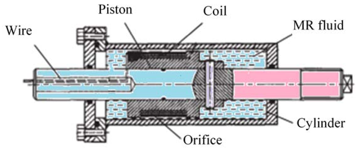
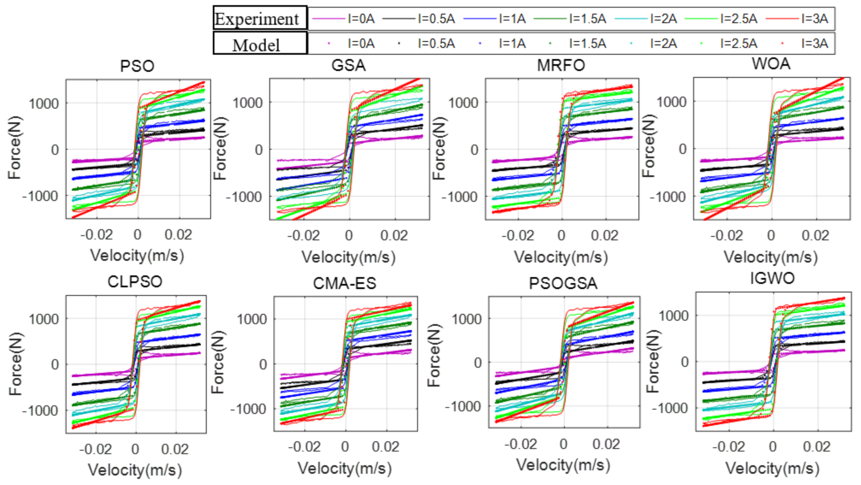
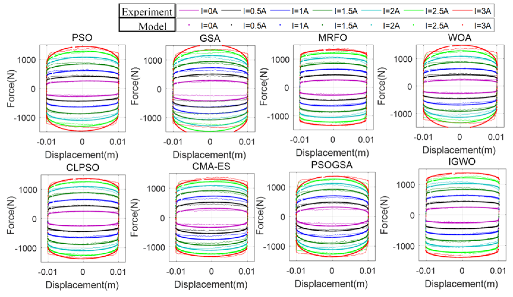
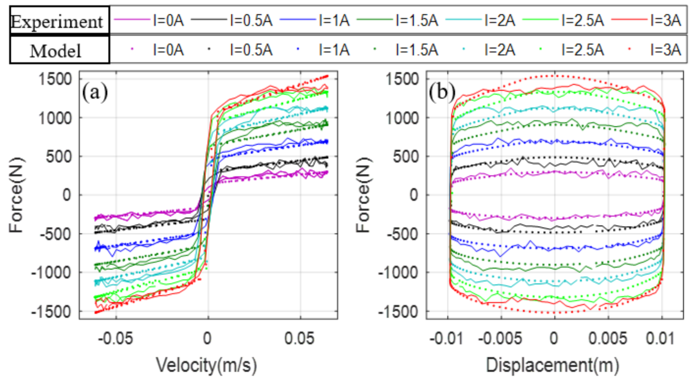
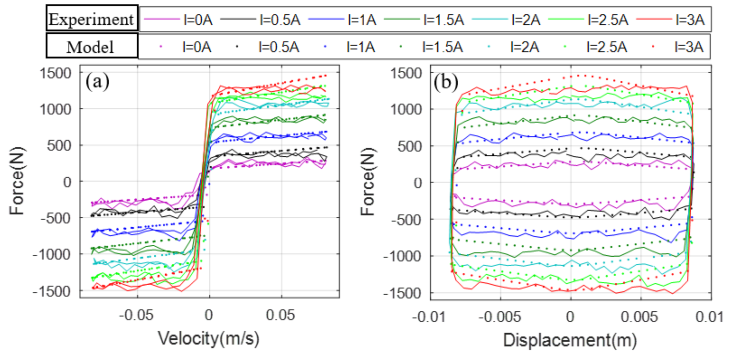
The Bouc–Wen model is established under various working conditions; the results discover that the IMRFO is more successful than its competitors in identifying the control parameters of the MR models.

The rest of this paper is organized as follows: Section 2 briefly introduces the basic MRFO, and Section 3 describes the proposed IMRFO algorithm in detail. The performance analysis of the IMRFO on benchmark functions is provided in Section 4. The experiment results and analysis for identifying the control parameters of MR dampers are presented in Section 5. Section 6 gives the conclusions and suggests a direction for future research.

2. Manta Ray Foraging Optimization (MRFO)

MRFO performs the optimization process by simulating the foraging behaviors of manta rays in nature to obtain the global optimum in the search space. MRFO has the following three foraging behaviors: chain foraging, cyclone foraging and somersault foraging. The chain foraging and somersault foraging behaviors contribute mainly to the exploitation search, while the cyclone foraging focuses on the exploration search. When solving an optimization problem using MRFO, the following update mechanisms are employed via the three foraging behaviors.

The chain foraging strategy of manta rays is as follows [42]:

$${\mathit{x}}_i(t+1)=\left\{\begin{array}{l}{\mathit{x}}_i\left(t\right)+r\cdot ({\mathit{x}}_{best}(t)-{\mathit{x}}_i(t\left)\right)+\alpha \cdot ({\mathit{x}}_{best}(t)-{\mathit{x}}_i(t))i=1\\ {\mathit{x}}_i\left(t\right)+r\cdot ({\mathit{x}}_{i-1}(t)-{\mathit{x}}_i(t\left)\right)+\alpha \cdot ({\mathit{x}}_{best}(t)-{\mathit{x}}_i(t))i=2,\cdots ,N\end{array}\right.$$

(1)

$$\alpha =2\cdot \mathit{r}\cdot \sqrt{|log(\mathit{r})|}$$

(2)

The cyclone foraging of manta rays is as follows [42]:

$${\mathit{x}}_i(t+1)=\left\{\begin{array}{l}{\mathit{x}}_{best}(t)+r\cdot ({\mathit{x}}_{best}(t)-{\mathit{x}}_i(t\left)\right)+\beta \cdot ({\mathit{x}}_{best}(t)-{\mathit{x}}_i(t))i=1\\ {\mathit{x}}_{best}(t)+r\cdot ({\mathit{x}}_{i-1}(t)-{\mathit{x}}_i(t\left)\right)+\beta \cdot ({\mathit{x}}_{best}(t)-{\mathit{x}}_i(t))i=2,\cdots ,N\end{array}\right.$$

(3)

$$\beta =2e^{r_1\frac{T-t+1}{T}}\cdot \sin (2\pi r_1)$$

(4)

and

$${\mathit{x}}_i(t+1)=\left\{\begin{array}{l}{\mathit{x}}_{rand}(t)+r\cdot ({\mathit{x}}_{rand}(t)-{\mathit{x}}_i(t\left)\right)+\beta \cdot ({\mathit{x}}_{rand}(t)-{\mathit{x}}_i(t))i=1\\ {\mathit{x}}_{rand}(t)+r\cdot ({\mathit{x}}_{i-1}(t)-{\mathit{x}}_i(t\left)\right)+\beta \cdot ({\mathit{x}}_{rand}(t)-{\mathit{x}}_i(t))i=2,\cdots ,N\end{array}\right.$$

(5)

$${\mathit{x}}_{rand}(\mathit{t})=\mathit{L}\mathit{b}+\mathit{r}\cdot (\mathit{L}\mathit{b}-\mathit{U}\mathit{b})$$

(6)

The somersault foraging of manta rays is as follows [42]:

$${\mathit{x}}_i(t+1)={\mathit{x}}_i(t)+S\cdot (r_2\cdot {\mathit{x}}_{best}-r_3\cdot {\mathit{x}}_i(t\left)\right),i=1,\cdots ,N$$

(7)

where x_i(t) is the position of the ith individual at iteration t, r is a random vector in [0, 1], r₁, r₂ and r₃ are the random numbers in [0, 1], x_best(t) is the food with the highest concentration, x_rand(t) is a random position randomly produced in the search space, Lb and Ub are the lower and upper boundaries of the variables, respectively and T is the maximum number of iterations.

3. Improved Manta Ray Foraging Optimization (IMRFO)

In MRFO, in the exploitation phase, each individual updates its position with respect to the individual with the best fitness by adjusting the values of α and β, which results in the decrease in the population diversity and stagnation in the local optima; meanwhile, the lack of fine-tuning ability also causes weak solution stability. To overcome these disadvantages, an improved MRFO, named IMRFO, is proposed. In MRFO, the value of t/T is employed to balance exploratory and exploitative searches, and the exploration probability of 0.25 indicates the weak exploration ability of the algorithm; therefore, a searching control factor is proposed in the IMRFO to improve the searching progress and exploration process. To enhance the search efficiency of the algorithm, an adaptive weight coefficient with the Levy flight is introduced in the algorithm, which can maximize the diversification of individuals and maintain the balance between population diversity and concentration. To avoid prematurely converging to local optima and a guaranteed solution stability, the Morlet wavelet mutation with the fine-tuning ability is incorporated into the algorithm.

3.1. Searching Control Factor

In MRFO, in the whole iteration process, there is a probability of 50% to perform the cyclone foraging in which the first half of searches contribute to exploration, according to the value of t/T. This is, the probability of exploration is only 25% and the relatively low probability happens in the first half of the optimization process, indicating the weak exploration ability of MRFO. In regard to this weak exploration, the searching behavior of MRFO is controlled by the value of t/T, which increases linearly as the iterations rise; however, in the IMRFO algorithm, the searching ability of the algorithm is controlled by a coefficient, p_s, called the searching control factor, which not only enables the algorithm to perform exploration with high probability in the second half of the optimization process but also makes it possible for the algorithm to perform exploration in the second half of the optimization process. The searching control factor p_s is defined as follows:

$$p_s(t)=(1-\frac{t}{T})\sqrt{\frac{5}{r}}$$

(8)

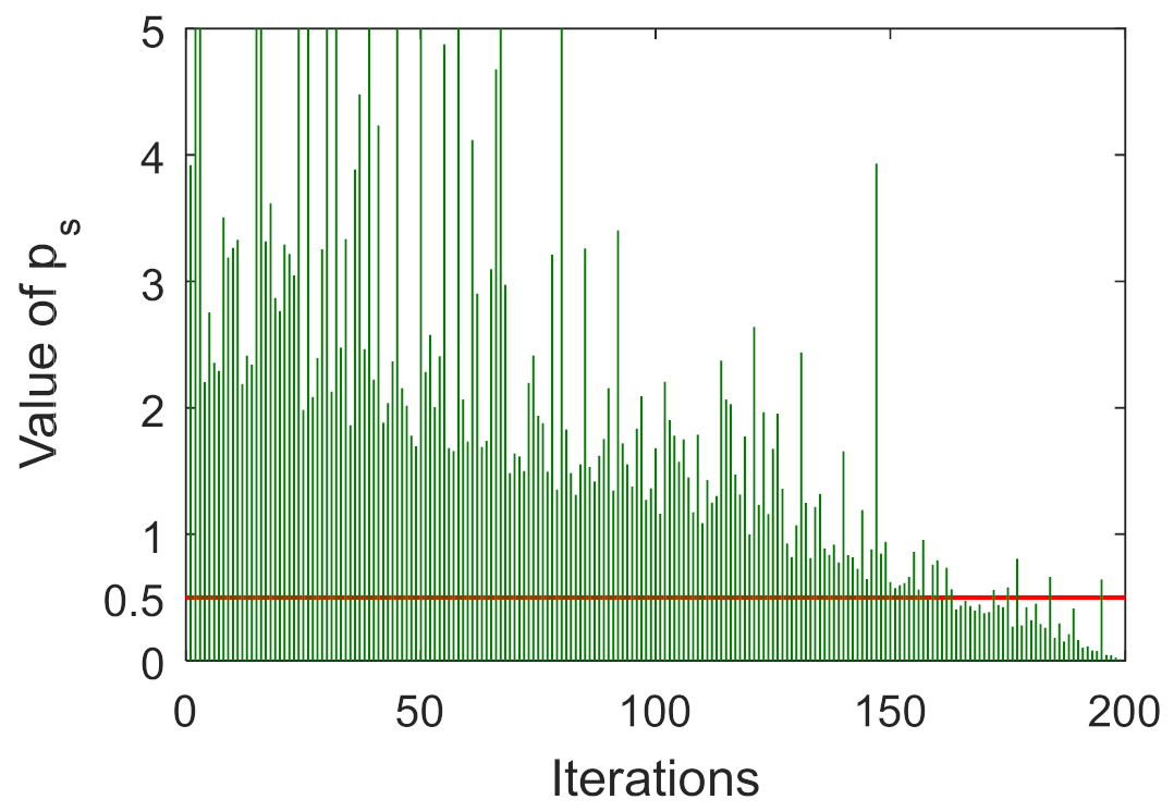
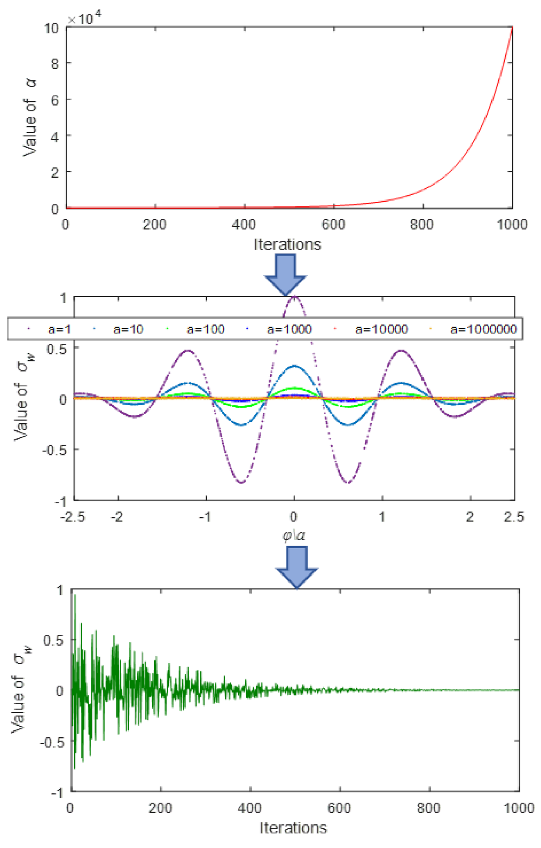
where r is the random number in the interval (0, 1]. Figure 1 gives the time-dependent curve of the searching control factor. When p_s > 0.5, the IMRFO performs exploration; otherwise, the algorithm performs exploitation. Obviously, from Figure 1, the searching control factor shows a decreasing trend with random oscillation, which also obliges the algorithm to explore the search in the later iteration.

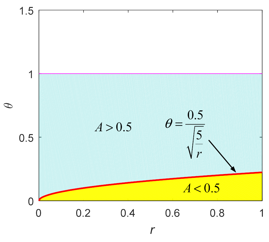
Let $\theta =1-\frac{t}{T}$, then $p_s(t)=\sqrt{\frac{5}{r}}\cdot \theta$, the probability of p_s > 0.5 is given by the following:

$$P\{A(t)>0.5\}=1-\frac{{\displaystyle \underset{0}{\overset{\frac{1}{2\sqrt{5}}}{\int }}{\displaystyle \underset{\frac{5}{{(\frac{0.5}{\theta })}^2}}{\overset{1}{\int }}drd\theta }}}{1\times 1}\approx 0.8509$$

(9)

Therefore, the probability of exploration in the IMRFO algorithm is 0.5 × 0.8509 = 0.4254 over the course of optimization. Figure 2 depicts the schematic diagram of the exploration probability of the algorithm based on the searching control factor p_s. Hence, the global exploration of the algorithm can be improved from 25 to 42.54% through the searching control factor p_s.

3.2. Adaptive Weight Coefficient with Levy Flight

Levy flight, as a simulation for the foraging activities of creatures, has been developed as an efficient search mechanism for an unknown space; therefore, it is widely employed to promote the search efficiency of various meta-heuristics [61,62,63,64,65,66]. In this part, using the fat-tailed characteristic producing numerous short steps punctuated by a few long steps from the Levy flight to construct a non-local random search mechanism, we can improve the search behavior in the cyclone foraging strategy of MRFO, which can effectively promote the diversity of search individuals and prevent the premature convergence of local optima.

The random step length of the Levy flight is offered by the following Levy distribution [66]:

$$L(s)\sim t^{-\lambda }(1\le \lambda \le 3)$$

(10)

where λ is a stability/tail index, and s is the step length. According to Mantegna’s algorithm [66], the step length of the Levy flight is given as follows:

$$s=\frac{u}{|v{|}^{\frac{1}{\beta }}}$$

(11)

where u and v obey the normal distribution, respectively. That is:

$$u\sim N(0,{\sigma }_u^2),v\sim N(0,1)$$

(12)

$${\sigma }_u={\left(\frac{\Gamma (1+\beta )\cdot \sin (\frac{\pi \beta }{2})}{\Gamma (\frac{1+\beta }{2})\cdot \beta \cdot 2^{\frac{\beta -2}{2}}}\right)}^{\frac{1}{\beta }}$$

(13)

Γ is the standard Gamma function and the default value of β is set to 1.5.

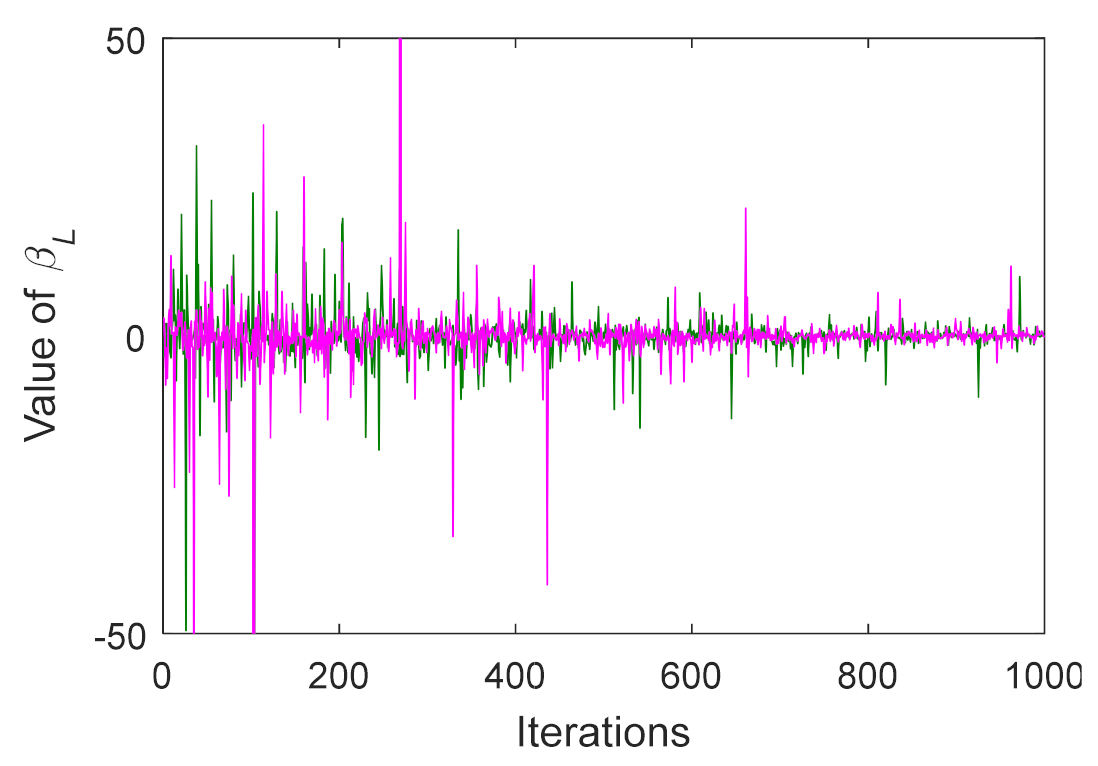
Therefore, an adaptive weight coefficient with the Levy flight in the cyclone foraging strategy is designed as follows:

$${\beta }_L=e^{\frac{2(T-t+1)}{T}}\cdot \frac{u}{2|v{|}^{\frac{1}{\beta }}}$$

(14)

Observing Equation (14), on the one hand, the multiple short steps produced frequently by the Levy flight promote the exploitation capacity, while the long steps produced occasionally enhance the exploration capacity, guaranteeing the local optima avoidance of the algorithm; on the other hand, $e^{\frac{2(T-t+1)}{T}}$ is a decreasing function with the iterations, depending on the decreasing trend of this function. A larger search scope is provided during the early iterations, while a smaller search scope is provided in the later iterations, this characteristic can promote the search efficiency of the algorithm and prevent the step lengths going out of the boundaries of the variables. The behavior of β_L during two runs with 1000 iterations is demonstrated in Figure 3.

The cyclone foraging of the IMRFO algorithm can be given as follows:

$${\mathit{x}}_i^d(t+1)=\left\{\begin{array}{l}{\mathit{x}}_{best}+r\cdot ({\mathit{x}}_{best}(t)-{\mathit{x}}_i(t\left)\right)+{\beta }_L\cdot ({\mathit{x}}_{best}(t)-{\mathit{x}}_i(t))\hspace{1em}i=1\\ {\mathit{x}}_{best}+r\cdot ({\mathit{x}}_{i-1}(t)-{\mathit{x}}_i(t\left)\right)+{\beta }_L\cdot ({\mathit{x}}_{best}(t)-{\mathit{x}}_i(t))\hspace{1em}i=2,\cdots ,N\end{array}\right.\hspace{1em}{p}_s<0.5$$

(15)

$${\mathit{x}}_i^d(t+1)=\left\{\begin{array}{l}{\mathit{x}}_{rand}+r\cdot ({\mathit{x}}_{rand}-{\mathit{x}}_i(t\left)\right)+{\beta }_L\cdot ({\mathit{x}}_{rand}-{\mathit{x}}_i(t))\hspace{1em}i=1\\ {\mathit{x}}_{rand}+r\cdot ({\mathit{x}}_{i-1}(t)-{\mathit{x}}_i(t\left)\right)+{\beta }_L\cdot ({\mathit{x}}_{rand}-{\mathit{x}}_i(t))\hspace{1em}i=2,\cdots ,N\end{array}\right.\hspace{1em}{p}_s\ge 0.5$$

(16)

3.3. Wavelet Mutation Strategy

It is easy for MRFO to trap into local optima, which results in an ineffective search for the global optimum and the instability of solutions. To improve the ability of the algorithm to step out of stagnation and the convergence rate and the stability of solutions, the Morlet wavelet mutation is incorporated into the somersault foraging strategy in the IMRFO algorithm. The wavelet mutation indicates that a dynamic adjustment of the mutation is implemented by combining the translations and dilations of a wavelet function [66,67]. To meet the fine-tuning purpose, the dilation parameters of the wavelet function are controlled to reduce its amplitude, which results in a constrain on the mutation space as the iterations increase.

Assume that p_m is the mutation probability, r₄ is a random number in [0, 1]. By incorporating the wavelet mutation, the somersault foraging strategy is improved by the following:

$${\mathit{x}}_i(t+1)=\left\{\begin{array}{l}\left\{\begin{array}{l}{\mathit{x}}_i\left(t\right)+{\sigma }_w\cdot ({\mathit{x}}_i(t)-Low)\hspace{1em}{\sigma }_w<0\\ {\mathit{x}}_i\left(t\right)+{\sigma }_w\cdot (Up-{\mathit{x}}_i(t))\hspace{1em}{\sigma }_w\ge 0\end{array}\right.\hspace{1em}\hspace{1em}{r}_4<p_m\\ {\mathit{x}}_i\left(t\right)+S\cdot (r_2\cdot {\mathit{x}}_{best}-r_3\cdot {\mathit{x}}_i(t\left)\right)\hspace{1em}\hspace{1em}\hspace{1em}\hspace{1em}{r}_4\ge p_m\end{array}\right.$$

(17)

where p_m is the mutation probability that is set to 0.1, and σ_w is the dilation parameters of a wavelet function, which can be given as follows:

$${\sigma }_w=\frac{1}{\sqrt{a}}\psi (\frac{{\phi }_i}{a})$$

(18)

where $\psi (x)$ is the Morlet wavelet function and it is defined as follows:

$$\psi (x)=e^{-\frac{x^2}{2}}\cos (5x)$$

(19)

More than 99% of the total energy of the wavelet function is contained in [−2.5, 2.5]. Thus, σ_w can be randomly generated from [−2.5a, 2.5a] [67]. a is the dilation parameter, which increases from 1 to s as the number of iterations increases. To avoid missing the global optimum, a monotonic increasing function can be given as follows [67]:

$$a=e^{-\ln (g)\cdot (1-\frac{t}{T})+\ln (g)}$$

(20)

where g is a constant number that is set to 100,000. The calculation of the Morlet wavelet mutation is visualized in Figure 4. From Figure 4, the value of the dilation parameter increases with the decrease in t, and thus, the amplitude of the Morlet wavelet function is decreased, which gradually reduces the significance of the mutation; this merit can ensure that the algorithm jumps out of local optima and improves the precision of the solutions. Moreover, the overall positive and negative mutations are nearly the same during the iteration process, and this property also ensures good solution stability.

3.4. The Proposed IMRFO Algorithm

In the IMRFO, the improvements for MRFO consist of the following three parts: first, a searching control factor is designed according to a weak exploration ability of MRFO, which can effectively increase the global exploration of the algorithm; second, to prevent the premature convergence of the local optima, an adaptive weight coefficient based on the Levy flight is designed to promote the search efficiency of the algorithm; three, the Morlet wavelet mutation strategy is introduced to the algorithm, in which the mutation space is adaptively adjusted according to the energy concentration of the wavelet function, it is helpful for the algorithm to step out of stagnation and speed up the convergence rate. In the IMRFO, in the somersault foraging, when the condition of r₄ < p_m is met, the Morlet wavelet mutation strategy is performed. The dilation parameters of a wavelet function σ_w is calculated according to the position of the individual x_i via Equations (18)–(20), and then the position of the individual is updated with respect to the upper boundary or lower boundary of the search space, according to the sign of σ_w (negative or positive) based on Equation (20). By this means, the Morlet wavelet mutation strategy is well integrated to the algorithm.

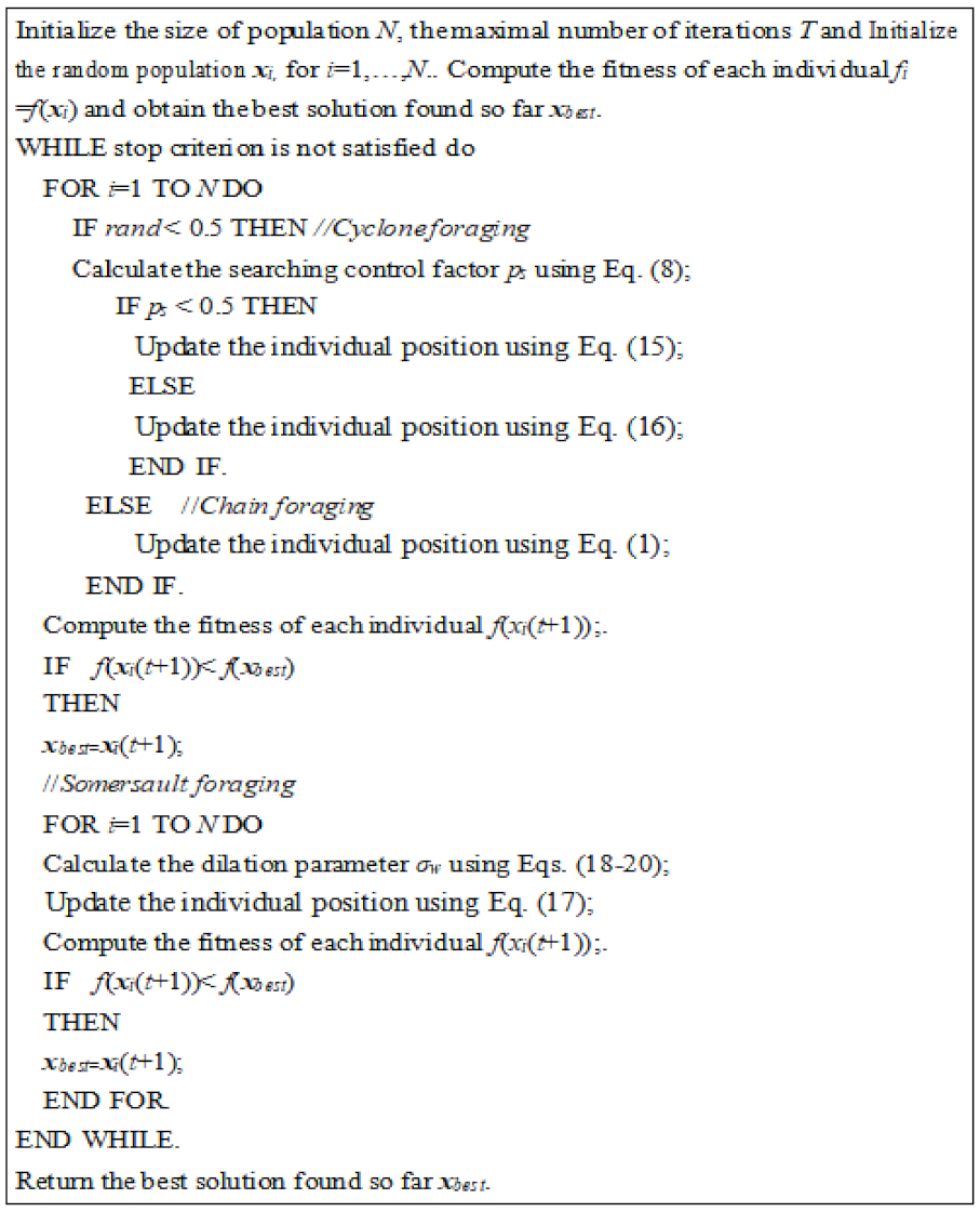
The pseudocode of the IMRFO algorithm is given in Figure 5, and the specific steps are as follows:

Step1: The related parameters of the IMRFO are initialized, such as the size of population, N, the maximum number of iterations, T and the mutation probability, p_m.

Step2: The initial population is randomly produced {x₁(0), x₂(0), …, x_N(0)}, the fitness of each individual is evaluated and the best solution x*(0) is restored.

Step3: If t ≤ T, for each individual in the population x_i(t), i = 1, …, N, if the condition of rand < 0.5 is met, the searching control factor p_s is calculated according to Equation (8).

Step 4: All the individuals are sorted according to their fitness from small to large and the adaptive weight coefficient is calculated according to Equations (10)–(14); if p_s < 0.5, the individual position is updated according to Equation (15), otherwise, the individual position is updated according to Equation (16); if the condition of rand < 0.5 is not met, the individual position is updated according to Equation (1).

Step 5: The individual that is out of the boundaries is relocated in the search space; the fitness value for each individual is evaluated and the best solution found thus far, x*(t), is restored.

Step 6: For each individual in the population x_i(t), the dilation parameter σ_w is calculated according to Equations (18)–(20), and the individual position is updated according to Equation (17).

Step 7: The individual that is out of the boundaries is relocated in the search space; the fitness value for each individual is evaluated and the best solution found thus far, x*(t), is restored.

Step 8: If the stop criterion is met, the best solution found thus far, x*(t), is restored; otherwise, set t = t + 1 and go to Step 3.

4. Experimental Analysis and Results

To analyze the performance of the IMRFO algorithm, a set of benchmark functions are employed in this study. This function suite contains the following three types: unimodal (UF), multimodal (MF) and composite (CF) functions. The UF functions (f1–f7) are able to check the exploitation ability of the algorithms and the MF functions (f8–f13) are able to reveal the exploration ability of the algorithms. The CF functions (f14–f21) are selected from the CEC 2014 benchmark suite [68], which are often employed in many optimization algorithms and can check the balance ability between exploration and exploitation. Details of these benchmark problems are described in the literature [69,70]. The performance of the IMRFO is compared with that of other optimization methods. These comparative optimizers in this study include: PSO, as the most popular swarm-based algorithm; GSA, as the most well-known physics-based algorithm; WOA and MRFO, as recent optimizers; comprehensive learning particle swarm optimizer (CLPSO) [71] and evolution strategy with covariance matrix adaptation (CMA-ES) [72], as highly effective optimizers; and PSOGSA and improved grey wolf optimization (IGWO) [7], as recent improved meta-heuristics with high performance.

For all the considered optimizers, the swarm size and maximum fitness evaluations (FEs) are set to 50 and 25,000, respectively. All the results of the algorithms are based on the average performance of 30 independent runs. The parameter settings of all the algorithms are given in

Table 1. Parameter settings for each algorithm.

Algorithm	Parameter	Value
PSO	Inertia weight; acceleration coefficients	Decrease from 0.9 to 0.4; 2,2
GSA	Gravitational constant; decreasing coefficient	100; 20
WOA	Convergence parameter	Decrease from 2 to 0
CMA-ES	Expected initial distance to optimum per coordinate	5
CLPSO	Inertia weight; acceleration coefficients	Decrease from 0.9 to 0.4; 1.49445, 1.49445
PSOGSA	Gravitational constant; decreasing coefficient; weighting factors	1; 20; 0.5, 1.5
IGWO	a	Decrease from 2 to 0
IMRFO	Mutation probability	0.1

.

4.1. Exploitation Evaluation

Table 2. Results provided algorithms for UF functions.

Fun.	Dim.	Index	PSO	GSA	MRFO	WOA	CLPSO	CMA-EA	PSOGSA	IGWO	IMRFO
f1	10	Mean	1.38 × 10−13	3.26 × 10−18	2.07 × 10−215	9.62 × 10−91	2.31 × 10−14	1.12 × 10−42	2.28 × 10−20	1.50 × 10−34	7.22 × 10−208
		STD	2.81 × 10−13	1.50 × 10−18	0	3.46 × 10−90	1.50 × 10−4	1.41 × 10−42	7.27 × 10−21	4.35 × 10−34	0
	30	Mean	2.63	3.44 × 10−17	4.08 × 10−207	1.08 × 10−83	1.74 × 102	7.93 × 10−10	1.00 × 103	2.73 × 10−15	8.50 × 10−199
		STD	2.90	1.03 × 10−17	0	5.38 × 10−83	51.7	5.42 × 10−10	3.05 × 103	3.07 × 10−15	0
	50	Mean	4.45 × 102	27.1	3.23 × 10−209	2.01 × 10−80	3.03 × 103	3.48 × 10−5	5.14 × 103	3.61 × 10−10	2.90 × 10−199
		STD	1.61 × 102	32.2	0	1.10 × 10−79	4.55 × 102	1.82 × 10−5	6.62 × 103	2.51 × 10−10	0
f2	10	Mean	6.70 × 10−9	5.37 × 10−9	1.47 × 10−110	7.45 × 10−56	1.46 × 10−3	3.58 × 10−21	3.18 × 10−10	2.93 × 10−21	2.18 × 10−104
		STD	8.09 × 10−9	1.21 × 10−9	4.19 × 10−110	3.86 × 10−55	5.51 × 10−4	1.54 × 10−21	5.22 × 10−11	4.00 × 10−21	6.59 × 10−104
	30	Mean	1.21 × 10−1	3.35 × 10−8	1.05 × 10−106	6.52 × 10−55	4.19	5.49 × 10−5	11.2	8.18 × 10−10	4.01 × 10−101
		STD	5.44 × 10−2	5.85 × 10−9	4.48 × 10−106	2.09 × 10−54	5.56 × 10−1	1.77 × 10−5	25.7	4.24 × 10−10	2.15 × 10−100
	50	Mean	4.15	1.32 × 10−1	3.83 × 10−107	1.17 × 10−51	30.1	9.99 × 10−3	51.2	7.55 × 10−7	1.15 × 10−101
		STD	1.09	2.74 × 10−1	1.58 × 10−106	6.12 × 10−51	3.19	2.16 × 10−3	47.1	4.33 × 10−7	3.81 × 10−101
f3	10	Mean	5.23 × 10−3	4.30	1.08 × 10−209	45.8	1.22 × 102	2.31 × 10−33	1.67 × 102	3.39 × 10−15	1.89 × 10−198
		STD	8.29 × 10−3	6.81	0	69.3	65.5	4.30 × 10−33	9.13 × 102	1.13 × 10−14	0
	30	Mean	8.72 × 103	5.28 × 102	1.56 × 10−202	2.78 × 104	1.75 × 104	3.64 × 10−1	1.32 × 104	3.06 × 10−1	9.86 × 10−191
		STD	4.34 × 103	2.29 × 102	0	1.00 × 104	2.84 × 103	3.83 × 10−1	5.97 × 103	4.21 × 10−1	0
	50	Mean	3.83 × 104	1.82 × 103	4.00 × 10−203	1.47 × 105	6.55 × 104	5.23 × 102	3.91 × 104	2.15 × 102	2.94 × 10−186
		STD	1.15 × 104	5.36 × 102	0	2.90 × 104	7.82 × 103	1.95 × 103	1.34 × 104	2.32 × 102	0
f4	10	Mean	5.58 × 10−4	1.19 × 10−9	5.31 × 10−109	1.96	8.83	2.21 × 10−19	3.15 × 10−1	3.81 × 10−11	5.49 × 10−102
		STD	4.43 × 10−4	2.51 × 10−10	1.20 × 10−108	5.81	1.51	9.91 × 10−20	1.19	4.35 × 10−11	2.78 × 10−101
	30	Mean	25.2	3.73	1.34 × 10−105	27.8	39.5	6.68 × 10−4	53	2.98 × 10−3	2.60 × 10−99
		STD	5.12	1.33	3.60 × 10−105	28.8	2.48	2.05 × 10−4	23.8	1.75 × 10−3	9.43 × 10−99
	50	Mean	47.7	8.54	4.71 × 10−104	53.8	53.5	9.07 × 10−2	77.5	2.11 × 10−1	4.93 × 10−98
		STD	5.38	1.82	2.15 × 10−103	33.0	2.95	4.18 × 10−2	14.9	1.07 × 10−1	1.30 × 10−97
f5	10	Mean	5.92	18.1	2.18	6.30	27.5	3.04 × 10−2	3.02 × 103	3.86	4.49 × 10−2
		STD	1.00	32.8	3.87 × 10−1	3.43 × 10−1	12	1.15 × 10−2	1.64 × 104	6.57 × 10−1	1.77 × 10−1
	30	Mean	8.81 × 102	39.0	24.1	27.3	4.22 × 104	20.0	73.8	25.1	4.12 × 10−5
		STD	7.60 × 102	32.7	4.77 × 10−1	4.54 × 10−1	1.52 × 104	7.11 × 10−1	66.7	7.94 × 10−1	7.76 × 10−13
	50	Mean	3.11 × 105	2.92 × 102	44.7	47.9	9.66 × 105	57.3	5.37 × 106	46.5	1.27 × 10−3
		STD	2.35 × 105	1.66 × 102	4.11 × 10−1	5.04 × 10−1	2.33 × 105	37.1	2.03 × 107	1.46	2.40 × 10−3
f6	10	Mean	0	0	0	0	0	0	6.33 × 10−1	0	0
		STD	0	0	0	0	0	0	8.09 × 10−1	0	0
	30	Mean	6.93	1.67 × 10−1	0	0	1.50 × 102	0	1.84 × 103	0	0
		STD	3.53	3.79 × 10−1	0	0	31.3	0	3.30 × 103	0	0
	50	Mean	4.98 × 102	1.40 × 102	0	0	2.68 × 103	0	9.03 × 103	0	0
		STD	2.89 × 102	84.9	0	0	4.25 × 102	0	7.13 × 103	0	0
f7	10	Mean	4.52 × 103	5.92 × 10−3	1.73 × 10−4	1.28 × 103	6.87 × 10−3	1.78 × 10−3	1.31 × 10−2	7.56 × 10−4	1.46 × 10−4
		STD	2.14 × 10−3	3.03 × 10−3	1.62 × 10−4	1.06 × 10−3	3.30 × 10−3	8.04 × 10−4	8.82 × 10−3	5.87 × 10−4	1.34 × 10−4
	30	Mean	1.23 × 10−1	2.91 × 10−2	1.97 × 10−4	2.36 × 10−3	1.61 × 10−1	7.23 × 10−3	1.14 × 10−1	3.86 × 10−3	1.75 × 10−4
		STD	4.94 × 10−2	1.01 × 10−2	1.43 × 10−4	3.18 × 10−3	3.76 × 10−2	2.52 × 10−3	4.72 × 10−2	1.47 × 10−3	1.95 × 10−4
	50	Mean	1.23	1.15 × 10−1	2.28 × 10−4	2.60 × 10−3	1.11	1.20 × 10−2	4.33 × 10−1	6.79 × 10−3	1.73 × 10−4
		STD	4.13 × 10−1	4.92 × 10−2	1.39 × 10−4	3.08 × 10−3	2.86 × 10−1	3.30 × 10−3	1.48 × 10−1	2.07 × 10−3	1.80 × 10−4

shows the results provided by the IMRFO and other optimizers in tackling UF functions f1–f7 with different dimensions. Inspecting Table 2, the IMRFO is very competitive with other optimizers on UF functions. In particular, there are significant improvements on functions f5 and f7 for all the dimensions. For the other UF functions, the IMRFO provides almost the same results as MRFO, followed by other algorithms. Therefore, the present algorithm is very effective in exploiting around the optimum and, thus, ensures a good exploitation ability.

4.2. Exploration Evaluation

The MF functions with numerous local optima are useful to evaluate the exploration ability of the algorithms.

Table 3. Results provided algorithms for MF functions.

Fun.	Dim.	Index	PSO	GSA	MRFO	WOA	CLPSO	CMA-EA	PSOGSA	IGWO	IMRFO
f8	10	Mean	−2.87 × 103	−1.70 × 103	−3.63 × 103	−3.36 × 103	−3.94 × 103	−2.50 × 103	−3.00 × 103	−3.96 × 103	−4.17 × 103
		STD	2.44 × 102	3.40 × 102	2.60 × 102	5.83 × 102	7.97 × 102	1.86 × 102	2.83 × 102	2.70 × 102	3.55 × 102
	30	Mean	−5.00 × 103	−2.76 × 103	−8.58 × 103	−1.09 × 104	−1.07 × 104	−4.39 × 103	−7.75 × 103	−7.86 × 103	−1.11 × 104
		STD	6.35 × 102	4.32 × 102	6.28 × 102	1.47 × 103	2.94 × 102	3.07 × 102	1.16 × 103	1.79 × 103	1.70 × 103
	50	Mean	−6.11 × 103	−3.66 × 103	−1.29 × 104	−1.79 × 104	−1.44 × 104	−5.74 × 103	−1.19 × 104	−9.28 × 103	−1.89 × 104
		STD	4.83 × 102	6.84 × 102	8.46 × 102	2.85 × 103	5.03 × 102	3.42 × 102	1.04 × 103	3.47 × 103	2.79 × 103
f9	10	Mean	4.02	3.32	0	1.67	1.99 × 10−1	13.5	35.1	5.73	0
		STD	1.89	13.7	0	6.45	1.82 × 10−1	9.12	15.0	5.71	0
	30	Mean	56.1	17.0	0	5.68 × 10−15	60.9	1.64 × 102	1.37 × 102	45.7	0
		STD	17.4	4.27	0	2.29 × 10−14	8.65	9.17	29.0	47.1	0
	50	Mean	1.34 × 102	33.4	0	0	2.01 × 102	2.67 × 102	2.47 × 102	64.2	0
		STD	23.5	80.7	0	0	17.3	1.04 × 102	61.8	24.8	0
f10	10	Mean	1.73 × 10−7	2.47 × 10−9	8.88 × 10−16	4.20 × 10−15	1.42 × 10−2	1.01 × 10−15	1.99 × 10−1	9.53 × 10−15	8.88 × 10−16
		STD	2.44 × 10−7	5.15 × 10−10	0	2.07 × 10−15	5.39 × 10−3	6.49 × 10−16	5.33 × 10−1	3.32 × 10−15	0
	30	Mean	1.35	4.91 × 10−9	8.88 × 10−16	4.68 × 10−15	6.57	9.11 × 10−6	12.9	1.04 × 10−8	8.88 × 10−16
		STD	6.57 × 10−1	9.60 × 10−10	0	1.60 × 10−15	5.50 × 10−1	2.59 × 10−16	5.08	5.84 × 10−9	0
	50	Mean	5.57	1.52 × 10−1	8.88 × 10−16	3.61 × 10−15	11.4	1.31 × 10−3	17.6	2.91 × 10−6	8.88 × 10−16
		STD	7.47 × 10−1	3.25 × 10−1	0	2.59 × 10−15	4.45 × 10−1	3.18 × 10−4	1.49	1.12 × 10−6	0
f11	10	Mean	9.67 × 10−2	1.68	0	6.48 × 10−2	5.47 × 10−2	0	1.69 × 10−1	3.33 × 10−2	0
		STD	5.16 × 10−2	1.20	0	1.08 × 10−1	2.54 × 10−2	0	8.21 × 10−2	2.32 × 10−2	0
	30	Mean	9.03 × 10−1	16.3	0	0	2.72	5.16 × 10−9	12.8	4.28 × 10−3	0
		STD	2.14 × 10−1	3.84	0	0	5.36 × 10−1	2.98 × 10−9	31.1	8.30 × 10−3	0
	50	Mean	5.21	1.02 × 102	0	3.70 × 10−18	26.9	2.63 × 10−4	79.6	2.47 × 10−3	0
		STD	2.30	13.4	0	2.03 × 10−17	5.06	9.54 × 10−5	74.5	4.74 × 10−3	0
f12	10	Mean	1.22 × 10−14	5.58 × 10−20	1.04 × 10−2	2.00 × 10−3	2.75 × 10−5	4.71 × 10−32	4.88 × 10−1	1.89 × 10−6	1.46 × 10−27
		STD	1.84 × 10−14	2.55 × 10−20	5.68 × 10−2	5.91 × 10−3	1.82 × 10−5	1.67 × 10−47	1.13	5.29 × 10−7	7.04 × 10−27
	30	Mean	6.35	4.70 × 10−1	2.83 × 10−8	7.01 × 10−3	8.70	6.00 × 10−11	8.94	1.14 × 10−2	4.10 × 10−11
		STD	3.56	4.28 × 10−1	2.94 × 10−8	4.61 × 10−3	2.11	5.93 × 10−11	4.98	2.03 × 10−2	5.56 × 10−11
	50	Mean	1.19 × 105	1.79	3.31	1.23 × 10−2	1.85 × 104	9.57 × 10−7	2.56 × 107	5.96 × 10−2	1.21 × 10−7
		STD	2.30 × 105	6.28 × 10−1	1.93 × 10−5	9.72 × 10−3	1.93 × 104	4.03 × 10−7	7.81 × 107	3.37 × 10−2	1.51 × 10−7
f13	10	Mean	1.11 × 10−13	2.87 × 10−19	2.03 × 10−2	2.80 × 10−3	2.44 × 10−4	1.35 × 10−32	7.32 × 10−4	9.87 × 10−6	1.46 × 10−3
		STD	2.25 × 10−13	1.02 × 10−13	4.07 × 10−2	3.92 × 10−3	1.96 × 10−4	5.57 × 10−48	2.79 × 10−3	3.69 × 10−6	3.80 × 10−3
	30	Mean	25.1	2.07	2.47	1.74 × 10−1	1.36 × 102	4.20 × 10−10	38.1	2.24 × 10−1	7.32 × 10−4
		STD	21.4	2.97	1.11	1.35 × 10−1	1.77 × 102	3.37 × 10−10	9.54	1.23 × 10−1	2.79 × 10−3
	50	Mean	4.62 × 105	28.8	4.92	5.12 × 10−1	6.18 × 105	2.30 × 10−5	5.47 × 107	1.41	5.10 × 10−6
		STD	5.08 × 105	10.3	1.26 × 10−1	2.32 × 10−1	2.84 × 105	1.03 × 10−5	1.42 × 108	3.08 × 10−1	1.89 × 10−5

gives the results provided by the IMRFO and other optimizers in tackling MF functions f8–f13 with different dimensions. From Table 3, the IMRFO performs the best for 50 dimensions of all the MF functions, the IMRFO offers the best results for 10 dimensions of the MF functions but functions f12 and f13, and the IMRFO outperforms all the other methods for 30 dimensions of the MF functions but function f13. Therefore, the IMRFO provides excellent results on these MF functions and its performance remains consistently superior for different dimensions of 10, 30 and 50. Obviously, these superior results benefit significantly from the high exploration ability of the IMRFO. This is due to the fact that the searching control factor increases the number of exploring the search space and the Morlet wavelet mutation strategy improves the exploration ability of the algorithm.

4.3. Evaluation of Local Optima Avoidance

Composite functions are the most challenging test suite; therefore, they are specifically used for evaluating the local optima avoidance of algorithms, which results from a proper balance between exploration and exploitation [73]. The results provided by the IMRFO and other optimizers in tackling CF functions f14–f21 are presented in

Table 4. The results provided algorithms for CF functions.

Fun.	Index	PSO	GSA	MRFO	WOA	CLPSO	CMA-EA	PSOGSA	IGWO	IMRFO
f14	Mean	2647.81	2578.60	2500.00	2681.93	2638.70	2706.03	2634.00	2617.82	2500.00
	STD	9.03	117.43	0	18.63	4.64	148.00	8.61	0.82	0
f15	Mean	2633.48	2620.13	2600.00	2608.33	2654.29	2617.53	2669.75	2600.26	2600.00
	STD	7.73	1.73	0	8.38	2.32	51.64	20.49	0.20	0
f16	Mean	2727.81	2706.18	2700.00	2725.71	2723.21	2713.20	2717.14	2707.26	2700.00
	STD	10.95	2.13	0	20.59	3.46	0.99	9.14	1.98	0
f17	Mean	2702.91	2795.25	2700.57	2710.46	2703.67	2704.87	2771.20	2700.50	2700.52
	STD	0.97	15.31	0.12	31.58	0.68	0.87	48.48	0.09	0.09
f18	Mean	3508.11	4624.61	2900.01	3740.09	3331.54	3680.23	3708.63	3195.69	2900.00
	STD	229.02	216.01	0.04	424.55	80.25	90.59	125.38	84.77	0
f19	Mean	7322.83	5455.38	3000.00	5693.72	5155.90	7452.47	4669.26	3849.98	3000.00
	STD	622.89	751.15	0	623.81	370.96	707.92	526.87	132.40	0
f20	Mean	3.07 × 107	2.77 × 106	3614.61	1.14 × 107	3.34 × 106	1.59 × 108	7.15 × 106	2.18 × 104	3586.18
	STD	2.91 × 107	6.45 × 106	718.74	9.34 × 106	1.77 × 106	6.19 × 107	6.62 × 106	8529.33	635.79
f21	Mean	1.43 × 105	2.06 × 106	9110.49	3.46 × 105	1.22 × 105	985,119.84	31,366.18	1.30 × 104	6905.11
	STD	1.81 × 105	8.58 × 105	2684.13	1.92 × 105	3.86 × 104	6.26 × 105	2.70 × 104	3389.18	1818.54

. Based on Table 4, the results from the IMRFO are not inferior to those from other algorithms except function f17. For function f17, the results from the IMRFO are second only to those of IGWO. The IMRFO can considerably outperform other algorithms and provide the best results for 87.5% of f14–f21 problems. It can be seen that the results of the IMRFO are again significantly better than other optimizers. Therefore, the results from Table 4 confirm that the IMRFO benefits from a good balance between exploratory and exploitative searches that assist the optimizer to effectively avoid local optima.

4.4. Convergence Evaluation

The convergence curves by the IMRFO and other optimizers in tackling the UF and MF functions are depicted in Figure 6, Figure 7, Figure 8, Figure 9 and Figure 10 to observe the convergence performance of the optimizers. The convergence curves provided in these figures are based on the mean of the best-so-far solutions in each iteration over 30 runs. It can be found that these curves share common characteristics: in the early stage of iterations, there are high fluctuations in the curves; the convergence rate tends to be accelerated as the iterations increase; in the later phase of iterations, the curves exhibit low variations. From the figure, compared to other algorithms, the convergence rate of the IMRFO tends to be speeded up with the increase in the iterations. This is owing to the Morlet wavelet mutation strategy for MRFO that enables the algorithm to search for the promising regions of the search space in the initial iterations and converge towards the global optimum more rapidly in the subsequent iterations. Overall, these convergence characteristics are attributed to the improved strategies in the IMRFO, by which the individuals of the population are able to effectively search the variable space and update their positions towards the global optimum solution. Thus, the excellent convergence performance of the IMRFO reveals that the algorithm achieves a better balance between exploitation and exploration than other algorithms in the optimization process.

4.5. CEC 2017 Benchmarking

To further comprehensively investigate the performance of the IMRFO, a set of challenging functions CEC 2017 [74] is employed in this experiment. The comparative optimizers are the same as in the previous experiment and their parameters are set to be the same as mentioned in Table 1. The results are based on 30 independent runs of each algorithm with the population size of 50 and FEs of 50,000.

To investigate the significance difference of the performance of the IMRFO versus other algorithms and whether the IMRFO statistically outperforms other algorithms when solving optimization tasks, a Wilcoxon Signed-Rank Test (WSRT) is used. In this experiment, the WSRT is performed at 5% level of significance [75]. The WSRT results between the IMRFO and other optimizers are listed in

Table 5. WSRT results between IMRFO and PSO, GSA, MRFO and WOA.

Fun.	PSO vs. IMRFO				GSA vs. IMRFO				MRFO vs. IMRFO				WOA vs. IMRFO
	p-Value	T+	T−	Winner	p-Value	T+	T−	Winner	p-Value	T+	T−	Winner	p-Value	T+	T−	Winner
F1	1.73 × 10−6	0	465	+	2.83 × 10−4	56	409	+	3.72 × 10−5	433	32	−	1.73 × 10−6	0	465	+
F2	1.73 × 10−6	0	465	+	1.73 × 10−6	0	465	+	1.73 × 10−6	0	465	+	1.73 × 10−6	0	465	+
F3	1.73 × 10−6	0	465	+	1.73 × 10−6	0	465	+	8.94 × 10−4	71	394	+	1.73 × 10−6	0	465	+
F4	1.73 × 10−6	0	465	+	1.73 × 10−6	0	465	+	2.61 × 10−4	55	410	+	1.73 × 10−6	0	465	+
F5	4.28 × 10−1	194	271	=	2.13 × 10−6	2	463	+	3.29 × 10−1	280	185	=	1.73 × 10−6	0	465	+
F6	9.59 × 10−1	230	235	=	1.92 × 10−6	1	464	+	8.19 × 10−5	41	424	+	1.73 × 10−6	0	465	+
F7	3.72 × 10−5	433	32	−	3.39 × 10−1	279	186	=	6.16 × 10−4	399	66	−	1.92 × 10−6	1	464	+
F8	3.71 × 10−1	276	189	=	1.06 × 10−1	154	311	=	3.49 × 10−1	278	187	=	4.29 × 10−6	9	456	+
F9	2.99 × 10−1	283	182	=	6.32 × 10−5	38	427	+	7.51 × 10−5	40	425	+	1.73 × 10−6	0	465	+
F10	2.60 × 10−6	4	461	+	4.72 × 10−2	136	329	+	2.37 × 10−5	27	438	+	1.73 × 10−6	0	465	+
F11	1.73 × 10−6	0	465	+	1.73 × 10−6	0	465	+	1.59 × 10−3	386	79	−	1.73 × 10−6	0	465	+
F12	1.73 × 10−6	0	465	+	1.73 × 10−6	0	465	+	1.73 × 10−6	0	465	+	1.73 × 10−6	0	465	+
F13	7.04 × 10−1	214	251	=	7.71 × 10−4	69	396	+	1.73 × 10−6	0	465	+	1.73 × 10−6	0	465	+
F14	9.32 × 10−6	17	448	+	1.73 × 10−6	0	465	+	1.74 × 10−4	50	415	+	1.73 × 10−6	0	465	+
F15	4.99 × 10−3	96	369	+	6.16 × 10−3	66	399	+	6.34 × 10−6	13	452	+	1.92 × 10−6	1	464	+
F16	1.73 × 10−6	0	465	+	1.73 × 10−6	0	465	+	1.85 × 10−2	118	347	+	1.73 × 10−6	0	465	+
F17	1.65 × 10−1	165	300	=	1.73 × 10−6	0	465	+	2.37 × 10−5	27	438	+	2.88 × 10−6	5	460	+
F18	2.88 × 10−6	5	460	+	3.16 × 10−3	89	376	+	5.98 × 10−2	141	324	=	2.88 × 10−6	5	460	+
F19	3.82 × 10−1	190	275	=	1.73 × 10−6	0	465	+	1.73 × 10−6	0	465	+	1.73 × 10−6	0	465	+
F20	1.85 × 10−2	347	118	−	1.73 × 10−6	0	465	+	5.44 × 10−1	203	262	=	2.60 × 10−6	4	461	+
F21	2.37 × 10−5	27	438	+	1.73 × 10−6	0	465	+	3.39 × 10−1	186	279	=	1.73 × 10−6	0	465	+
F22	2.84 × 10−5	29	436	+	1. × 10−6	0	465	+	1.04 × 10−3	73	392	+	1.73 × 10−6	0	465	+
F23	1.73 × 10−6	0	465	+	1.73 × 10−6	0	465	+	4.20 × 10−4	61	404	+	2.35 × 10−6	3	462	+
F24	1.73 × 10−6	0	465	+	1.73 × 10−6	0	465	+	3.11 × 10−5	30	435	+	1.73 × 10−6	0	465	+
F25	1.73 × 10−6	0	465	+	1.73 × 10−6	0	465	+	1.74 × 10−4	50	415	+	1.73 × 10−6	0	465	+
F26	2.37 × 10−5	27	438	+	1.73 × 10−6	0	465	+	2.11 × 10−3	382	83	−	4.29 × 10−6	9	456	+
F27	1.73 × 10−6	0	465	+	1.73 × 10−6	0	465	+	3.71 × 10−1	189	276	=	2.35 × 10−6	3	462	+
F28	1.73 × 10−6	0	465	+	1.73 × 10−6	0	465	+	3.88 × 10−6	8	457	+	1.73 × 10−6	0	465	+
F29	8.47 × 10−6	16	449	+	1.73 × 10−6	0	465	+	5.29 × 10−4	64	401	+	1.73 × 10−6	0	465	+
+/=/−	20/7/2				27/2/0				19/6/4				29/0/0

. In Table 5 and

Table 6. WSRT results between IMRFO and CLPSO, CMA-ES, PSOGSA and IGWO.

Fun.	CLPSO vs. IMRFO				CMA-ES vs. IMRFO				PSOGSA vs. IMRFO				IGWO vs. IMRFO
	p-Value	T+	T−	Winner	p-Value	T+	T−	Winner	p-Value	T+	T−	Winner	p-Value	T+	T−	Winner
F1	1.73 × 10−6	0	465	+	8.94 × 10−4	71	394	+	2.16 × 10−5	26	439	+	1.73 × 10−6	0	465	+
F2	1.73 × 10−6	0	465	+	1.73 × 10−6	0	465	+	1.73 × 10−6	0	465	+	1.73 × 10−6	0	465	+
F3	1.73 × 10−6	0	465	+	1.73 × 10−6	0	465	+	1.73 × 10−6	0	465	+	2.05 × 10−4	52	413	+
F4	1.73 × 10−6	0	465	+	1.74 × 10−4	50	415	+	6.98 × 10−6	14	451	+	3.33 × 10−2	129	336	+
F5	1.41 × 10−1	304	161	=	7.51 × 10−5	40	425	+	1.92 × 10−6	1	464	+	1.59 × 10−3	386	79	−
F6	1.73 × 10−6	465	0	−	5.32 × 10−3	97	368	+	3.52 × 10−6	7	458	+	1.73 × 10−6	465	0	−
F7	3.72 × 10−5	433	32	−	4.07 × 10−5	432	33	−	9.32 × 10−6	17	448	+	3.88 × 10−6	457	8	−
F8	1.41 × 10−1	304	161	=	1.04 × 10−3	73	392	+	1.24 × 10−5	20	445	+	1.36 × 10−5	444	21	−
F9	3.39 × 10−1	279	186	=	3.72 × 10−5	433	32	−	1.73 × 10−6	0	465	+	1.73 × 10−6	465	0	−
F10	1.24 × 10−5	20	445	+	1.73 × 10−6	0	465	+	1.96 × 10−3	82	383	+	9.71 × 10−5	43	422	+
F11	1.73 × 10−6	0	465	+	1.73 × 10−6	0	465	+	1.73 × 10−6	0	465	+	1.38 × 10−3	77	388	+
F12	1.73 × 10−6	0	465	+	1.73 × 10−6	0	465	+	1.13 × 10−5	19	446	+	2.13 × 10−6	2	463	+
F13	1.73 × 10−6	0	465	+	1.73 × 10−6	0	465	+	6.32 × 10−5	38	427	+	1.92 × 10−6	1	464	+
F14	1.73 × 10−6	0	465	+	1.73 × 10−6	0	465	+	1.92 × 10−6	1	464	+	3.11 × 10−6	30	435	+
F15	2.88 × 10−6	5	460	+	1.73 × 10−6	0	465	+	1.83 × 10−3	81	384	+	1.02 × 10−5	18	447	+
F16	9.10 × 10−1	227	238	=	2.60 × 10−6	4	461	+	1.97 × 10−5	25	440	+	1.36 × 10−1	305	160	=
F17	2.26 × 10−3	381	84	−	1.32 × 10−2	112	353	+	3.18 × 10−6	6	459	+	1.49 × 10−5	443	22	−
F18	3.11 × 10−5	30	435	+	2.60 × 10−6	4	461	+	5.29 × 10−4	64	401	+	5.71 × 10−4	65	400	+
F19	2.60 × 10−6	4	461	+	1.73 × 10−6	0	465	+	4.20 × 10−4	61	404	+	1.32 × 10−2	112	353	+
F20	8.94 × 10−4	394	71	−	3.88 × 10−6	8	457	+	2.88 × 10−6	5	460	+	6.34 × 10−6	452	13	−
F21	1.83 × 10−3	81	384	+	1.73 × 10−6	0	465	+	1.73 × 10−6	0	465	+	2.77 × 10−3	378	87	−
F22	2.16 × 10−5	26	439	+	9.59 × 10−1	235	230	=	4.29 × 10−6	9	456	+	1.97 × 10−5	25	440	+
F23	2.89 × 10−1	181	284	=	1.73 × 10−6	0	465	+	1.73 × 10−6	0	465	+	2.41 × 10−4	411	54	−
F24	5.71 × 10−4	65	400	+	1.73 × 10−6	0	465	+	4.29 × 10−6	9	456	+	1.80 × 10−5	441	24	−
F25	1.73 × 10−6	0	465	+	2.71 × 10−1	286	179	=	9.71 × 10−6	43	422	+	1.96 × 10−3	82	383	+
F26	2.21 × 10−1	292	173	=	4.29 × 10−6	9	456	+	1.74 × 10−4	50	415	+	1.29 × 10−3	389	76	−
F27	2.77 × 10−3	378	87	−	1.73 × 10−6	0	465	+	5.58 × 10−1	204	261	=	1.73 × 10−6	465	0	−
F28	1.73 × 10−6	0	465	+	4.99 × 10−3	96	369	+	1.73 × 10−6	0	465	+	2.35 × 10−6	3	462	+
F29	4.65 × 10−1	197	268	=	1.53 × 10−1	163	302	=	1.13 × 10−5	19	446	+	6.89 × 10−5	426	39	−
+/=/−	17/7/5				24/3/2				28/1/0				15/1/13

, ‘=’ signifies that there is no significant difference between the IMRFO and other algorithms, ‘+’ signifies that the null hypothesis is rejected and the IMRFO outperforms other ones and ‘−’ vice versa. The statistical results of ‘=’, ‘−’ and ‘+’ for all the algorithms are given in the last row of each table. From Table 5 and Table 6, it can be observed that there is a statistical significance difference between the IMRFO and other optimizers and the performance of the IMRFO is superior to the other eight competitive optimizers on the majority of test tasks.

To further evaluate the difference between the IMRFO and its counterparts and rank them statistically, another statistical test, the Friedman Test (FT), is employed based on the average performance of the algorithms in this study. The performance ranks of the FT for each of the 29 functions among all the considered algorithms are given in

Table 7. Performance rank of algorithms for each function.

Fun.	IMRFO	PSO	GSA	MRFO	WOA	CLPSO	CMA-EA	PSOGSA	IGWO
F1	2	6	5	1	7	4	9	8	3
F2	1	6	7	2	4	5	8	9	3
F3	1	4	6	2	9	7	8	5	3
F4	1	8	5	2	6	4	9	7	3
F5	2	4	6	5	9	3	7	8	1
F6	3	5	7	4	9	2	6	8	1
F7	6	2	5	7	8	3	4	9	1
F8	2	4	6	5	8	3	9	7	1
F9	5	4	7	6	9	3	2	8	1
F10	1	8	3	2	7	5	9	4	6
F11	2	4	8	1	9	5	7	6	3
F12	1	6	5	2	7	4	9	8	3
F13	1	7	3	2	5	6	9	8	4
F14	1	5	8	3	9	6	7	4	2
F15	1	6	3	2	8	7	9	4	5
F16	2	7	6	3	8	4	9	5	1
F17	3	5	9	4	7	2	6	8	1
F18	1	6	4	2	8	5	7	9	3
F19	2	3	6	1	9	5	7	8	4
F20	4	3	9	5	7	2	6	8	1
F21	2	5	8	3	7	4	9	6	1
F22	1	3	8	2	9	6	4	7	5
F23	2	7	9	4	6	3	8	5	1
F24	2	7	9	3	6	4	8	5	1
F25	1	8	6	3	7	4	5	9	2
F26	3	5	7	4	8	2	9	6	1
F27	4	7	9	3	6	2	8	5	1
F28	1	8	7	2	5	4	9	6	3
F29	2	6	9	4	8	3	5	7	1

and their ranks, on average, are depicted in Figure 11, in which the lower rank denotes the better algorithm. Regarding the results in Table 7, the IMRFO can achieve the best results on 12 functions; a WOA can achieve the best results on 3 functions; and an IGWO can achieve the best results on 14 functions. Observing Figure 11, the IMRFO offers the lowest rank of all the comparative algorithms, indicating that the IMRFO can achieve the best performance, followed by IGWO, MRFO and CLPSO. Consequently, this statistical test proves the effectiveness and superiority of the combination of those strategies proposed in the IMRFO.

5. Optimal Parameter Identification of MR Damper

5.1. Principle of Operation

The MR damper is a kind of intelligent semi-active control device; controlling the size of the coil in the current instructions can change the strength of the magnetic field, which directly affects the viscosity coefficient of magnetorheological fluids, thus working to control the outputs of the damper. The general structure of the MR damper is plotted in Figure 12 [76]. The MR fluid is enclosed in a cylinder and flows through a small orifice; meanwhile, a magnetizing coil is enclosed in the piston. When a current is fed to the coil, the particles suspended in the MR fluid are aligned, this enables the fluid to change from the liquid state to the semisolid state within milliseconds, thus generating a controllable damping force.

The mechanical performance test of the MR damper is carried out on the tensile test bed. The experimental platform uses the amplitude signals of different frequencies from the exciter and the current provided by the MR shimmy damper, which are employed to generate some data signals, i.e., the damping force and cylinder rod displacement. The sinusoidal signals are used to generate the excitation in the MR damper, which can be expressed as follows:

$$x=A\sin (2\pi ft)$$

(21)

where x is the displacement of the damper piston, A is the amplitude of signals, f is the frequency of signals and t is the time. When the amplitude and frequency of the signals are constant, the displacements versus time for the different loading currents can be generated. Therefore, the dynamic responses of the MR damper, i.e., damping force–displacement and damping force–velocity, can be obtained by test data processing under various operating conditions. Figure 13 shows the typical damping force–displacement and damping force–velocity test curves for the amplitude A = 10 mm and frequency f = 0.5 Hz [76].

5.2. Bouc–Wen Model

Various MR models had been proposed to reproduce the dynamic responses of the MR damper, among which the Bouc–Wen model is one of the most commonly employed models owing to its good hysteretic characteristics and strong universality [77]; the Bouc–Wen model is depicted in Figure 14.

The mechanical behavior of the Bouc–Wen model is described as follows:

$$F=c_0\dot{x}+k_0(x-x_0)+\alpha z$$

(22)

$$\dot{z}=-\gamma \left|\dot{x}\right|z|z{|}^{n-1}-\beta \dot{x}z|z{|}^n+A\dot{x}$$

(23)

where x is the damper displacement, c₀ is the damping coefficient of a dashpot, x₀ is the initial deflection of spring with the stiffness k₀, z is the hysteretic variable and, α, β, γ and n are the model parameters of the MR damper, which are given as follows [76]:

$$\alpha ={\alpha }_{\alpha }I+{\alpha }_b$$

(24)

$$c_0=c_{0\alpha }e{c}_{0b}I$$

(25)

$$\beta ={\beta }_{\alpha }e{\beta }_{b}I$$

(26)

$$A=A_{\alpha }{I}^2+A_{b}I+A_c$$

(27)

The following 15 parameters need to be determined in our study:

$${\alpha }_b,c_{0\alpha },c_{0b},k_0,c_1,k_1,\gamma ,{\beta }_{\alpha },{\beta }_b,A_{\alpha },A_b,A_c,n,and{x}_0$$

When these parameters are determined, the output damping force needs to be calculated using the Bouc–Wen model. Therefore, the Bouc–Wen model is established using SIMULINK.

5.3. Simulation Results and Analysis

After the establishment of the model, a fitness function should be defined that can evaluate the quality of the model with the given parameters. Thus, in this study, the mean error rate (MER) between the simulation data and experimental data is employed as the following fitness function [76]:

$$f_{ER}^j=\sqrt{\frac{{\displaystyle \sum _{i=1}^m{(F_i^j-F_i^{*j})}^2}}{{\displaystyle \sum _{i=1}^m{(F_i^j-\frac{1}{m}{\displaystyle \sum _{i=1}^m{F}_i^j})}^2}}}$$

(28)

$$f_{MER}=\frac{1}{c}{\displaystyle \sum _{j=1}^c{f}^j}$$

(29)

where m is the number of damping forces, c is the number of the constant loading currents, $F_i^j$ and $F_i^{*j}$ are the ith experimental force and the ith simulation force from the model under the jth loading current, respectively and $f_{ER}^j$ is the error rate under a loading current. Therefore, to find the optimal model parameters, the proposed IMRFO algorithm is adopted, and the results are compared with those from the other optimizers.

The experimental data, i.e., the damper amplitude, velocity and the outputted damper force, are obtained under a wide range of operating conditions.

Table 8. Test operating conditions of Bouc–Wen model.

	Frequency (Hz)	Amplitude (mm)	Loading Current (A)
Case1	0.5	10	0	0.5	1	1.5	2	2.5	3
Case2	1	10
Case3	1.5	10

gives the test operating conditions. In Table 8, the working frequencies are set to 0.5, 1 and 1.5 Hz, while the amplitude is set 10 mm, respectively; moreover, the loading current is set from 0 to 3 A with the step length 0.5 A. Thus, there are three combination cases of frequency and displacement, and there are seven current types for each of the combination cases. For each case, the results offered by the IMRFO are compared with those offered by some other algorithms. For all the algorithms, the population size and the maximum FEs are set to 30 and 6000, respectively. For different loading currents, the search space of each parameter will be slightly different. For example, when I = 0.5 A, the search space of the 15 parameters is given as follows:

Lb = [10⁴, 10⁴, 10³, 10⁻², 100, 10⁶, 10², 10², 10³, −1, −10, −100, 100, 0.1, 10⁻⁴];

Ub = [10⁵, 10⁵, 10⁴, 1, 10³, 10⁷, 10³, 10⁴, 10⁴, −0.1, −1, −1, 10³, 1, 1].

Table 9. Results provided using different algorithms for three cases.

Fun.	Index	Objective Function (fMER)
		PSO	GSA	MRFO	WOA	CLPSO	CMA-EA	PSOGSA	IGWO	IMRFO
Case 1	Mean	1.091 × 10−1	2.343 × 10−1	1.345 × 10−1	7.345 × 10−2	1.877 × 10−1	7.896 × 10−2	1.478 × 10−1	7.402 × 10−2	6.706 × 10−2
	STD	9.035 × 10−2	1.145 × 10−2	2.290 × 10−3	3.010 × 10−3	6.465 × 10−3	2.185 × 10−3	3.800 × 10−3	5.897 × 10−4	2.238 × 10−4
Case 2	Mean	2.325 × 10−1	6.219 × 10−1	2.667 × 10−1	1.930 × 10−1	2.380 × 10−1	2.092 × 10−1	2.935 × 10−1	2.277 × 10−1	1.773 × 10−1
	STD	1.952 × 10−2	1.658 × 10−1	3.179 × 10−3	3.036 × 10−2	1.061 × 10−2	1.048 × 10−3	5.771 × 10−3	2.516 × 10−3	1.717 × 10−3
Case 3	Mean	2.655 × 10−1	7.154 × 10−1	2.667 × 10−1	2.387 × 10−1	2.380 × 10−1	2.535 × 10−1	2.935 × 10−1	2.277 × 10−1	2.275 × 10−1
	STD	6.687 × 10−2	4.544 × 10−2	2.850 × 10−2	6.458 × 10−2	8.677 × 10−2	5.653 × 10−2	3.634 × 10−2	3.596 × 10−2	1.004 × 10−2

lists the experimental results provided by the IMRFO and its competitors for three different cases. From Table 9, the IMRFO yields the most favorable performance in case one, in terms of ‘Mean’ and ‘Std’ followed by WOA, IGWO and CMA-ES; in case two, the IMRFO achieves the most reliable performance with comparison to other algorithms, followed by IGWO, PSOGSA and CLPSO; in case three, the IMRFO also offers better results than the other optimizers, followed by IGWO, WOA and CMA-EA. Therefore, Table 9 manifests that the IMRFO obtains more stable high-quality solutions than its counterparts when solving the Bouc–Wen model with different operating conditions. The 15 parameters of the Bouc–Wen are provided in

Table 10. Parameters of Bouc–Wen model for loading current = 0.5 A.

Parameters	PSO	GSA	MRFO	WOA	CLPSO	CMA-ES	PSOGSA	IGWO	IMRFO
${\alpha }_{\alpha }$	3.59 × 104	9.17 × 104	2.58 × 104	3.71 × 104	3.19 × 104	5.33 × 104	8.01 × 104	2.29 × 104	4.43 × 104
${\alpha }_b$	7.11 × 104	4.78 × 104	1.29 × 104	3.08 × 104	2.02 × 104	2.11 × 104	6.11 × 104	1.25 × 104	4.18 × 104
$c_{0\alpha }$	2.81 × 103	5.01 × 103	3.89 × 103	3.07 × 103	3.55 × 103	5.67 × 103	7.05 × 103	2.78 × 103	2.61 × 103
$c_{0b}$	6.19 × 10−1	4.95 × 10−1	1.77 × 10−1	6.87 × 10−1	4.36 × 10−1	1.90 × 10−1	3.26 × 10−1	3.37 × 10−1	4.83 × 10−1
$k_0$	8.45 × 102	2.46 × 102	2.10 × 102	2.38 × 102	2.87 × 102	5.84 × 102	1.77 × 102	7.76 × 102	8.70 × 102
$c_1$	6.21 × 106	9.60 × 106	5.16 × 106	6.67 × 106	3.86 × 106	7.31 × 106	1.00 × 106	5.64 × 106	4.61 × 106
$k_1$	6.55 × 102	2.05 × 102	2.82 × 102	3.38 × 102	1.05 × 102	2.77 × 102	1.33 × 102	1.59 × 102	1.26 × 102
$\gamma$	6.36 × 103	7.42 × 102	4.50 × 102	6.72 × 102	7.15 × 102	6.36 × 103	7.09 × 103	7.48 × 103	1.94 × 103
${\beta }_{\alpha }$	8.30 × 103	7.10 × 103	7.60 × 103	6.34 × 103	9.91 × 103	4.21 × 103	6.81 × 103	5.15 × 103	8.43 × 103
${\beta }_b$	−7.24 × 10−1	−2.25 × 10−1	−2.93 × 10−1	−8.85 × 10−1	−7.26 × 10−1	−4.29 × 10−1	−8.85 × 10−1	−3.63 × 10−1	−3.91 × 10−1
$A_{\alpha }$	−4.90	−1.31	−8.03	−3.21	−4.99	−1.05	−5.54	−2.98	−9.26
$A_b$	−47.8	−26.7	−17.8	−88.5	−35.9	−61.3	−86.0	−24.5	−34.2
$A_c$	4.55 × 102	2.13 × 102	3.92 × 102	6.91 × 102	3.50 × 102	5.22 × 102	9.35 × 102	4.08 × 102	3.89 × 102
$n$	5.49 × 10−1	7.67 × 10−1	7.66 × 10−1	5.52 × 10−1	7.81 × 10−1	6.02 × 10−1	4.20 × 10−1	7.96 × 10−1	6.02 × 10−1
$x_0$	9.86 × 10−3	3.24 × 10−1	2.35 × 10−2	7.01 × 10−2	1.63 × 10−2	2.09 × 10−2	1.00 × 10−4	7.83 × 10−3	1.42 × 10−2

using different algorithms for the loading current = 0.5 A.

The convergence curves of all the algorithms for the three cases are depicted in Figure 15. It can be observed that the IMRFO displays the highest convergence rate during the entire optimization process for cases one and two. For case three, the convergence rate of the IMRFO is significantly superior to the other competitors at the later optimization process. Moreover, the IMRFO offers the final solutions with the highest precision in the three cases, demonstrating its superior convergence performance for finding the optimum solution.

The comparisons between the experimental data and simulated results from the Bouc–Wen model using the parameters identified provided by the IMRFO are shown in Figure 16, in which the damping forces obtained from the experiment are plotted in solid lines, while the damping forces from the model are plotted in dots. From Figure 16, the damping force from the experimental data increases with the increase in the loading currents, and the increasing amplitude decreases gradually. Observing the damping force–displacement test curves and damping force–velocity test curves in Figure 16, for each of the different loading currents, the simulated data from the IMRFO-based Bouc–Wen model can agree well with the experimental data; these results show the effectiveness of the proposed method in identifying the damping parameters of the MR damper.

Figure 17 and Figure 18 show the comparison of the damping force–velocity and damping force–displacement test curves between the experimental data and the simulated results for case one using the other different algorithms, respectively. It can be seen from Figure 17 and Figure 18 that the matching contains some big discrepancies between the experimental data and the simulated data from the Bouc–Wen models provided by PSO, GSA, WOA, CLPSO, CMA-ES and PSOGSA. Although it is difficult to visually identify the matching quality among the IMRFO, MRFO and IGWO from these figures, the IMRFO is more competitive than the other methods from Table 9.

To verify whether the IMRFO-based Bouc–Wen model can reflect the mechanical properties of the MR damper, two extensive simulations, i.e., cases two and three, are performed by changing the frequency of the model. The comparisons between the experimental data and simulated data from the Bouc–Wen model using the parameters identified by the IMRFO for cases two and three are shown in Figure 19 and Figure 20, respectively; Figure 21 and Figure 22 show the comparison of the damping force–velocity test curves between the experimental data and the simulated data from the Bouc–Wen model using the parameters identified by the other different algorithms for cases two and three, respectively; and Figure 23 and Figure 24 show the comparison of the damping force–displacement test curves between the experimental data and the simulated data from the Bouc–Wen model using the parameters identified by the other different algorithms for cases two and three, respectively. These results reveal that the simulated data from the IMRFO-based model show better coincidence with the experimental data compared to its competitors, and the IMRFO-based model can accurately describe the dynamic performance of the MR damper with different frequencies.

To evaluate the matching performance of the MR damper models from different algorithms, an indicator named the mean Nash–Sutcliffe efficiency (MNSE) is employed; the MNSE is formulated as follows:

$$f_{NSE}^j=1-\frac{{\displaystyle \sum _{i=1}^m{(F_i^j-F_i^{*j})}^2}}{{\displaystyle \sum _{i=1}^m{(F_i^j-\frac{1}{m}{\displaystyle \sum _{i=1}^m{F}_i^j})}^2}}$$

(30)

$$f_{MNSE}=\frac{1}{c}{\displaystyle \sum _{j=1}^c{f}_{NSE}^j}$$

(31)

where $f_{NSE}^j$ is a single Nash–Sutcliffe efficiency (NSE) value under a given loading current. In general, the closer the value of the NSE is to one, the better the matching between the experimental data and simulated data from the model will be.

Figure 25, Figure 26 and Figure 27 show the matching comparison of the models based on different algorithms for cases 1–3 using the NSE, respectively. In these figures, the NSE of the models based on different algorithms under each of all the considered loading currents is depicted for each case, and the MNSE of the models based on each algorithm under all the considered loading currents is provided for each case. From Figure 25 (case one), the IMRFO-based model obtains the biggest NSE for each loading current and the MNSE compared to other competitors, demonstrating the superior matching performance of the model from our optimizer. Thus, the results of the NSE in Figure 25 show that the IMRFO-based model provides the best simulated results when tackling case one. From Figure 26, it can be found that the IMRFO-based model obtains the best matching performance measured using the NSE; the MRFO-based model is the second best, followed by the IGWO-based, CLPSO-based and PSOGSA-based models. Note that the model from GSA yields the worst matching performance in terms of the NSE, manifesting the model provides the unfavorable simulated data for case two. From Figure 27, for case three, the IMRFO-based model offers the most favorable matching performance that is almost the same as that offered by the IGWO-based model, followed by the PSOGSA-based, MRFO-based and CLPSO-based models.

Table 11. Matching results of models from different algorithms for cases 1–3.

	Mean Nash–Sutcliffe Efficiency (fMNSE)
	PSO	GSA	MRFO	WOA	CLPSO	CMA-EA	PSOGSA	IGWO	IMRFO
Case 1	0.987	0.933	0.981	0.993	0.963	0.993	0.975	0.994	0.995
Case 2	0.944	0.709	0.95	0.962	0.954	0.955	0.927	0.959	0.968
Case 3	0.926	0.477	0.928	0.942	0.942	0.935	0.909	0.947	0.947
Average of fMNSE	0.952	0.706	0.953	0.966	0.953	0.961	0.937	0.967	0.970

summarizes the matching results of the models from different algorithms for cases 1–3. From Table 11, the IMRFO-based model attains the results that are significantly better than, or almost the same as, the results of the models from the other eight peer algorithms for cases 1–3. Additionally, the average MNSE of the three cases from the IMRFO-based model outperforms that from the models based on the other algorithms, indicating the best overall performance of the IMRFO-based model. Based on the above analysis, the proposed IMRFO can provide superior and very competitive optimization performance in identifying the control parameters of the MR damper model.

In order to better evaluate the performance of the algorithm, we need to study not only the solution quality, but also the computational burden. Therefore, the running time of the IMRFO and its competitor are compared under identical conditions. The mean running time of the algorithms for cases 1–3 is given in

Table 12. Mean running time of different algorithms for cases 1–3.

Fun.	Mean Running Time (s)
	PSO	GSA	MRFO	WOA	CLPSO	CMA-EA	PSOGSA	IGWO	IMRFO
Case 1	1754	1820	1839	1815	1787	1893	1829	1838	1825
Case 2	1685	1730	1730	1716	1680	1746	1743	1774	1728
Case 3	1778	1946	1868	1847	1814	1879	1879	2003	1862

. From Table 12, each algorithm spends most of the time in executing SIMULINK. The mean running time of the IMRFO is very close to that of the other algorithms; there was no significant difference between the IMRFO and others in terms of running time; however, the solution quality of the IMRFO is significantly improved compared to the other methods.

6. Conclusions

In this study, a new hybrid MRFO is proposed for solving the global optimization and parameter identification of the MR damper models. In this improvement, the searching control factor is introduced to the algorithm to alleviate the weak exploration ability, and the adaptive weight coefficient is employed to promote the search efficiency of the algorithm. Additionally, the Morlet wavelet mutation strategy is integrated into the algorithm to enhance the ability of the algorithm to step out of stagnation and the convergence rate. Two sets of the challenging benchmarks, i.e., CEC 2014 and CEC 2017, are used to estimate the optimization performance of the IMRFO and the results demonstrate that the IMRFO is superior to the other algorithms. A comprehensive simulation based on the MR damper models is established, including three different test working conditions, in which 15 control parameters need to be identified using the proposed IMRFO algorithm. According to these identified parameters, the damping force–velocity and damping force–displacement test curves can be obtained, which show a highly satisfactory coincidence with the experimental data. Meanwhile, the comparison analysis shows that the IMRFO-based MR damper model can provide the best simulation results.

Eventually, the results of the benchmark functions and the optimal parameter identification of the MR damper model discover that the proposed optimizer has significant potential when solving engineering optimization problems. The Bouc–Wen damper model identified by the IMRFO is not only consistent with the experimental data involved in the simulation, but it can also accurately express the dynamic response of the Bouc–Wen damper model with different amplitudes and frequencies under sinusoidal excitation.

The IMRFO introduced improved strategies that achieve competitive performance verified by the benchmark experiments and the MR damper model. However, we have found out that there are two open problems that need to be further investigated in our future work. One issue is how to design an efficient adaptive strategy to adjust the movement step of individuals according to their neighborhoods’ solutions. Another issue is how to establish an information sharing mechanism to promote the searching efficiency. Moreover, in future work, it would be interesting to further extend the IMRFO to other complex MR damper models in which more different control parameters of the models need to be identified.

References

1. Tse, T.; Chang, C.C. Shear-mode rotary magnetorheological damper for small-scale structural control experiments. J. Struct. Eng. 2004, 130, 904–911. [Google Scholar] [CrossRef]
2. Liu, Y.Q.; Yang, S.P.; Liao, Y.Y. Simulation analysis on lateral semi-active control of suspension system for high-speed emus. J. Vib. Shock 2010, 29, 51–54. [Google Scholar]
3. Atabay, E.; Ozkol, I. Application of a magnetorheological damper modeled using the current–dependent bouc–wen model for shimmy suppression in a torsional nose landing gear with and without freeplay. J. Vib. Control 2014, 20, 1622–1644. [Google Scholar] [CrossRef]
4. Yang, S.; Li, S.; Wang, X.; Gordaninejad, F.; Hitchcock, G. A hysteresis model for magneto-rheological damper. Int. J. Nonlinear Sci. Numer. Simul. 2005, 6, 139–144. [Google Scholar] [CrossRef]
5. Xu, Z.D.; Xu, Y.W.; Wang, C.; Zhao, Y.L.; Ji, B.H.; Du, Y.L. Force tracking model and experimental verification on a novel magnetorheological damper with combined compensator for stay cables of bridge. Structures 2021, 32, 1971–1985. [Google Scholar] [CrossRef]
6. Yu, J.; Dong, X.; Su, X.; Qi, S. Development and characterization of a novel rotary magnetorheological fluid damper with variable damping and stiffness. Mech. Syst. Signal Process. 2022, 165, 108320. [Google Scholar] [CrossRef]
7. Boreiry, M.; Ebrahimi-Nejad, S.; Marzbanrad, J. Sensitivity analysis of chaotic vibrations of a full vehicle model with magnetorheological damper. Chaos Solitons Fractals 2019, 127, 428–442. [Google Scholar] [CrossRef]
8. Patel, D.M.; Upadhyay, R.V. Predicting the thermal sensitivity of MR damper performance based on thermo-rheological properties. Mater. Res. Express 2018, 6, 015707. [Google Scholar] [CrossRef]
9. Gołdasz, J.; Sapinski, B. Influence of Temperature on the MR Squeeze-Mode Damper. In Proceedings of the 2019 20th International Carpathian Control Conference (ICCC); IEEE: Krakow-Wieliczka, Poland, 2019; pp. 1–6. [Google Scholar]
10. Versaci, M.; Cutrupi, A.; Palumbo, A. A magneto-thermo-static study of a magneto-rheological fluid damper: A finite element analysis. IEEE Trans. Magn. 2020, 57, 1–10. [Google Scholar] [CrossRef]
11. Giuclea, M.; Sireteanu, T.; Stancioiu, D.; Stammers, C.W. Model parameter identification for vehicle vibration control with magnetorheological dampers using computational intelligence methods. Proc. Inst. Mech. Eng. Part I J. Syst. Control Eng. 2004, 218, 569–581. [Google Scholar] [CrossRef]
12. Gogna, A.; Tayal, A. Etaheuristics: Review and application. J. Exp. Theor. Artif. Intell. 2013, 25, 503–526. [Google Scholar] [CrossRef]
13. Kwok, N.M.; Ha, Q.P.; Nguyen, T.H.; Li, J.; Samali, B. A novel hysteretic model for magnetorheological fluid dampers and parameter identification using particle swarm optimization. Sens. Actuators A Phys. 2006, 132, 441–451. [Google Scholar] [CrossRef]
14. Gou, J.; Lei, Y.X.; Guo, W.P.; Wang, C.; Cai, Y.Q.; Luo, W. A novel improved particle swarm optimization algorithm based on individual difference evolution. Appl. Soft Comput. 2017, 57, 468–481. [Google Scholar] [CrossRef]
15. Zhao, W.; Shi, T.; Wang, L.; Cao, Q.; Zhang, H. An adaptive hybrid atom search optimization with particle swarm optimization and its application to optimal no-load PID design of hydro-turbine governor. J. Comput. Des. Eng. 2021, 8, 1204–1233. [Google Scholar]
16. Caselli, N.; Soto, R.; Crawford, B.; Valdivia, S.; Olivares, R. A self-adaptive cuckoo search algorithm using a machine learning technique. Mathematics 2021, 9, 1840. [Google Scholar] [CrossRef]
17. Zhao, W.; Wang, L.; Zhang, Z. A novel atom search optimization for dispersion coefficient estimation in groundwater. Future Gener. Comput. Syst. 2019, 91, 601–610. [Google Scholar] [CrossRef]
18. Soleimani Amiri, M.; Ramli, R.; Ibrahim, M.F.; Abd Wahab, D.; Aliman, N. Adaptive particle swarm optimization of PID gain tuning for lower-limb human exoskeleton in virtual environment. Mathematics 2020, 8, 2040. [Google Scholar] [CrossRef]
19. Mirjalili, S. Moth-flame optimization algorithm: A novel nature-inspired heuristic paradigm. Knowl.-Based Syst. 2015, 89, 228–249. [Google Scholar] [CrossRef]
20. Yang, X.S.; Gandomi, A.H. Bat algorithm: A novel approach for global engineering optimization. Eng. Comput. 2012, 29, 464–483. [Google Scholar] [CrossRef] [Green Version]
21. Jain, M.; Singh, V.; Rani, A. A novel nature-inspired algorithm for optimization: Squirrel search algorithm. Swarm Evol. Comput. 2019, 44, 148–175. [Google Scholar] [CrossRef]
22. Zhao, W.; Wang, L.; Zhang, Z. Artificial ecosystem-based optimization: A novel nature-inspired meta-heuristic algorithm. Neural Comput. Appl. 2019, 32, 1–43. [Google Scholar] [CrossRef]
23. Mirjalili, S.; Lewis, A. The whale optimization algorithm. Adv. Eng. Softw. 2016, 95, 51–67. [Google Scholar] [CrossRef]
24. Li, M.D.; Zhao, H.; Weng, X.W.; Han, T. A novel nature-inspired algorithm for optimization: Virus colony search. Adv. Eng. Softw. 2016, 92, 65–88. [Google Scholar] [CrossRef]
25. Pan, W.T. A new fruit fly optimization algorithm: Taking the financial distress model as an example. Knowl.-Based Syst. 2012, 26, 69–74. [Google Scholar] [CrossRef]
26. Arora, S.; Singh, S. Butterfly optimization algorithm: A novel approach for global optimization. Appl. Soft Comput. 2019, 23, 715–734. [Google Scholar] [CrossRef]
27. Dhiman, G.; Kumar, V. Spotted hyena optimizer: A novel bio-inspired based meta-heuristic technique for engineering applications. Adv. Eng. Softw. 2017, 114, 48–70. [Google Scholar] [CrossRef]
28. Saremi, S.; Mirjalili, S.; Lewis, A. Grasshopper optimisation algorithm: Theory and application. Adv. Eng. Softw. 2017, 105, 30–47. [Google Scholar] [CrossRef] [Green Version]
29. Yang, X.S. Flower pollination algorithm for global optimization. In Proceedings of the International Conference on Unconventional Computing and Natural Computation; Springer: Berlin/Heidelberg, Germany, 2012; pp. 240–249. [Google Scholar]
30. Askarzadeh, A. A novel meta-heuristic method for solving constrained engineering optimization problems: Crow search algorithm. Comput. Struct. 2016, 169, 1–12. [Google Scholar] [CrossRef]
31. Mirjalili, S.; Mirjalili, S.M.; Lewis, A. Grey wolf optimizer. Adv. Eng. Softw. 2014, 69, 46–61. [Google Scholar] [CrossRef] [Green Version]
32. EskandaR, H.; Sadollah, A.; Bahreininejad, A.; Hamdi, M. Water cycle algorithm-A novel metaheuristic optimization method for solving constrained engineering optimization problems. Comput. Struct. 2012, 110, 151–166. [Google Scholar] [CrossRef]
33. Rashedi, E.; Nezamabadi-Pour, H.; Saryazdi, S. GSA: A gravitational search algorithm. J. Inf. Sci. 2009, 179, 2232–2248. [Google Scholar] [CrossRef]
34. Zhao, W.; Wang, L.; Zhang, Z. Atom search optimization and its application to solve a hydrogeologic parameter estimation problem. Knowl.-Based Syst. 2019, 163, 283–304. [Google Scholar] [CrossRef]
35. Hashim, F.A.; Houssein, E.H.; Mabrouk, M.S.; Al-Atabany, W.; Mirjalili, S. Henry gas solubility optimization: A novel physics-based algorithm. Future Gener. Comput. Syst. 2019, 101, 646–667. [Google Scholar] [CrossRef]
36. Kaveh, A.; Talatahari, S. A novel heuristic optimization method: Charged system search. Acta Mech. 2010, 213, 267–289. [Google Scholar] [CrossRef]
37. Kaveh, A.; Bakhshpoori, T. Water evaporation optimization: A novel physically inspired optimization algorithm. Comput. Struct. 2016, 167, 69–85. [Google Scholar] [CrossRef]
38. Faramarzi, A.; Heidarinejad, M.; Stephens, B.; Mirjalili, S. Equilibrium optimizer: A novel optimization algorithm. Knowl.-Based Syst. 2020, 191, 105190. [Google Scholar] [CrossRef]
39. Zhao, W.; Wang, L.; Zhang, Z. Supply-demand-based optimization: A novel economics-inspired algorithm for global optimization. IEEE Access 2019, 7, 73182–73206. [Google Scholar] [CrossRef]
40. Molina, D.; Poyatos, J.; Del Ser, J.; García, S.; Hussain, A.; Herrera, F. Comprehensive taxonomies of nature-and bio-inspired optimization: Inspiration versus algorithmic behavior, critical analysis recommendations. Cogn. Comput. 2020, 12, 897–939. [Google Scholar] [CrossRef]
41. Črepinšek, M.; Liu, S.H.; Mernik, M. Replication and comparison of computational experiments in applied evolutionary computing: Common pitfalls and guidelines to avoid them. Appl. Soft Comput. 2014, 19, 161–170. [Google Scholar] [CrossRef]
42. Zhao, W.; Zhang, Z.; Wang, L. Manta ray foraging optimization: An effective bio-inspired optimizer for engineering applications. Eng. Appl. Artif. Intell. 2020, 87, 103300. [Google Scholar] [CrossRef]
43. Alhumade, H.; Fathy, A.; Al-Zahrani, A.; Rawa, M.J.; Rezk, H. Optimal parameter estimation methodology of solid oxide fuel cell using modern optimization. Mathematics 2021, 9, 1066. [Google Scholar] [CrossRef]
44. Ben, U.C.; Akpan, A.E.; Mbonu, C.C.; Ebong, E.D. Novel methodology for interpretation of magnetic anomalies due to two-dimensional dipping dikes using the Manta Ray Foraging Optimization. J. Appl. Geophys. 2021, 192, 104405. [Google Scholar] [CrossRef]
45. Shaheen, A.M.; Ginidi, A.R.; El-Sehiemy, R.A.; Ghoneim, S.S. Economic power and heat dispatch in cogeneration energy systems using manta ray foraging optimizer. IEEE Access 2020, 8, 208281–208295. [Google Scholar] [CrossRef]
46. Hemeida, M.G.; Ibrahim, A.A.; Mohamed, A.A.A.; Alkhalaf, S.; El-Dine, A.M.B. Optimal allocation of distributed generators DG based Manta Ray Foraging Optimization algorithm (MRFO). Ain Shams Eng. J. 2021, 12, 609–619. [Google Scholar] [CrossRef]
47. Eid, A.; Abdelaziz, A.Y.; Dardeer, M. Energy loss reduction of distribution systems equipped with multiple distributed generations considering uncertainty using manta-ray foraging optimization. Int. J. Renew. Energy Dev. 2021, 10, 779–787. [Google Scholar] [CrossRef]
48. Houssein, E.H.; Ibrahim, I.E.; Neggaz, N.; Hassaballah, M.; Wazery, Y.M. An efficient ECG arrhythmia classification method based on Manta ray foraging optimization. Expert Syst. Appl. 2021, 181, 115131. [Google Scholar] [CrossRef]
49. Duman, S.; Dalcalı, A.; Özbay, H. Manta ray foraging optimization algorithm–based feedforward neural network for electric energy consumption forecasting. Int. Trans. Electr. Energy Syst. 2021, e12999. [Google Scholar] [CrossRef]
50. Passino, K.M. Bacterial foraging optimization. Int. J. Swarm Intell. Res. IJSIR 2010, 1, 1–16. [Google Scholar] [CrossRef]
51. Turgut, O.E. A novel chaotic manta-ray foraging optimization algorithm for thermo-economic design optimization of an air-fin cooler. SN Appl. Sci. 2021, 3, 1–36. [Google Scholar] [CrossRef]
52. Houssein, E.H.; Emam, M.M.; Ali, A.A. Improved manta ray foraging optimization for multi-level thresholding using COVID-19 CT images. Neural Comput. Appl. 2021, 104827. [Google Scholar]
53. Ćalasan, M.P.; Jovanović, A.; Rubežić, V.; Mujičić, D.; Deriszadeh, A. Notes on parameter estimation for single-phase transformer. IEEE Trans. Ind. Appl. 2020, 56, 3710–3718. [Google Scholar] [CrossRef]
54. Hassan, M.H.; Houssein, E.H.; Mahdy, M.A.; Kamel, S. An improved manta ray foraging optimizer for cost-effective emission dispatch problems. Eng. Appl. Artif. Intell. 2021, 100, 104155. [Google Scholar] [CrossRef]
55. Elaziz, M.A.; Yousri, D.; Al-qaness, M.A.; AbdelAty, A.M.; Radwan, A.G.; Ewees, A.A. A Grunwald–Letnikov based Manta ray foraging optimizer for global optimization and image segmentation. Eng. Appl. Artif. Intell. 2021, 98, 104105. [Google Scholar] [CrossRef]
56. Elaziz, M.A.; Hosny, K.M.; Salah, A.; Darwish, M.M.; Lu, S.; Sahlol, A.T. New machine learning method for image-based diagnosis of COVID-19. PLoS ONE 2020, 15, e0235187. [Google Scholar] [CrossRef]
57. Jena, B.; Naik, M.K.; Panda, R.; Abraham, A. Maximum 3D Tsallis entropy based multilevel thresholding of brain MR image using attacking Manta Ray foraging optimization. Eng. Appl. Artif. Intell. 2021, 103, 104293. [Google Scholar] [CrossRef]
58. Yang, W.; Tang, G.; Hao, Y.; Wang, J. A novel framework for forecasting, evaluation and early-warning for the influence of PM10 on public health. Atmosphere 2021, 12, 1020. [Google Scholar] [CrossRef]
59. Ramadan, H.S.; Helmi, A.M. Optimal reconfiguration for vulnerable radial smart grids under uncertain operating conditions. Comput. Electr. Eng. 2021, 93, 107310. [Google Scholar] [CrossRef]
60. Houssein, E.H.; Zaki, G.N.; Diab, A.A.Z.; Younis, E.M. An efficient Manta Ray Foraging Optimization algorithm for parameter extraction of three-diode photovoltaic model. Comput. Electr. Eng. 2021, 94, 107304. [Google Scholar] [CrossRef]
61. Emary, E.; Zawbaa, H.M.; Sharawi, M. Impact of Lévy flight on modern meta-heuristic optimizers. Appl. Soft Comput. 2019, 75, 775–789. [Google Scholar] [CrossRef]
62. Hassan, M.H.; Kamel, S.; Selim, A.; Khurshaid, T.; Domínguez-García, J.L. A modified Rao-2 algorithm for optimal power flow incorporating renewable energy sources. Mathematics 2021, 9, 1532. [Google Scholar] [CrossRef]
63. Zhao, W.; Wang, L. Multiple-Kernel MRVM with LBFO algorithm for fault diagnosis of broken rotor bar in induction motor. IEEE Access 2019, 7, 182173–182184. [Google Scholar] [CrossRef]
64. Sun, Y.; Wang, X.; Chen, Y.; Liu, Z. A modified whale optimization algorithm for large-scale global optimization problems. Expert Syst. Appl. 2018, 114, 563–577. [Google Scholar] [CrossRef]
65. Viswanathan, G.M.; Afanasyev, V.; Buldyrev, S.V.; Murphy, E.J.; Prince, P.A.; Stanley, H.E. Lévy flight search patterns of wandering albatrosses. Nature 1996, 381, 413–415. [Google Scholar] [CrossRef]
66. Mantegna, R.N. Fast, accurate algorithm for numerical simulation of Levy stable stochastic processes. Phys. Rev. E 1994, 49, 4677–4683. [Google Scholar] [CrossRef] [PubMed]
67. Ling, S.H.; Lu, H.; Chan, K.Y.; Lam, H.K.; Yeung, B.; Leung, F.H. Hybrid particle swarm optimization with wavelet mutation and its industrial applications. IEEE transactions on systems, man and cybernetics. Part B Cybern. 2008, 38, 743–763. [Google Scholar] [CrossRef] [Green Version]
68. Guo, W.; Liu, T.; Dai, F.; Xu, P. An improved whale optimization algorithm for forecasting water resources demand. Appl. Soft Comput. 2019, 86, 105925. [Google Scholar] [CrossRef]
69. Liang, J.J.; Qu, B.Y.; Suganthan, P.N. Problem Definitions and Evaluation Criteria for the CEC 2014 Special Session and Competition on Single Objective Real-Parameter Numerical Optimization; Technical Report 201311; Nanyang Technological University: Singapore, 2013; Volume 635, p. 490. [Google Scholar]
70. Suganthan, P.N.; Hansen, N.; Liang, J.J.; Deb, K.; Chen, Y.P.; Auger, A.; Tiwari, S. Problem Definitions and Evaluation Criteria for the CEC 2005 Special Session on Real-Parameter Optimization; KanGAL Report 2005005; Nanyang Technological University: Singapore, 2005; pp. 1–50. [Google Scholar]
71. Liang, J.J.; Qin, A.K.; Suganthan, P.N.; Baskar, S. Comprehensive learning particle swarm optimizer for global optimization of multimodal functions. IEEE Trans. Evol. Comput. 2006, 10, 281–295. [Google Scholar] [CrossRef]
72. Hansen, N.; Müller, S.D.; Koumoutsakos, P. Reducing the time complexity of the derandomized evolution strategy with covariance matrix adaptation (CMA-ES). Evol. Comput. 2003, 11, 1–18. [Google Scholar] [CrossRef]
73. Nadimi-Shahraki, M.H.; Taghian, S.; Mirjalili, S. An improved grey wolf optimizer for solving engineering problems. Expert Syst. Appl. 2021, 166, 113917. [Google Scholar] [CrossRef]
74. Awad, N.H.; Ali, M.Z.; Liang, J.J.; Qu, B.Y.; Suganthan, P.N. CEC 2017 Special Session on Single Objective Numerical Optimization Single Bound Constrained Real-Parameter Numerical Optimization. 2017. Available online: https://www.researchgate.net/profile/Cholmin-Rim/publication/311671283_Adaptive_Niching_Chaos_Optimization_Algorithm_CEC_2017_Competition_on_Single_Objective_Real-Parameter_Numerical_Optimization/links/58d385f892851c319e570626/Adaptive-Niching-Chaos-Optimization-Algorithm-CEC-2017-Competition-on-Single-Objective-Real-Parameter-Numerical-Optimization.pdf (accessed on 6 September 2021).
75. Derrac, J.; García, S.; Molina, D.; Herrera, F. A practical tutorial on the use of nonparametric statistical tests as a methodology for comparing evolutionary and swarm intelligence algorithms. Swarm Evol. Comput. 2011, 1, 3–18. [Google Scholar] [CrossRef]
76. Liu, Y.Q.; Yang, S.P.; Liao, Y.Y. A quantizing method for determination of controlled damping parameters of magnetorheological damper models. J. Intell. Mater. Syst. Struct. 2011, 22, 2127–2136. [Google Scholar] [CrossRef]
77. Wen, Y.K. Method of random vibration of hysteretic systems. J. Eng. Mech. Div. ASCE 1976, 102, 249–263. [Google Scholar] [CrossRef]
Figure 1. Time−dependent curve of searching control factor.
Mathematics 09 02230 g001
Figure 2. Schematic diagram of exploration probability of the algorithm based on the searching control probability ps.
Mathematics 09 02230 g002
Figure 3. Value of βL during two runs with 1000 iterations.
Mathematics 09 02230 g003
Figure 4. Calculation of the Morlet wavelet mutation.
Mathematics 09 02230 g004
Figure 5. Pseudocode of IMRFO.
Mathematics 09 02230 g005
Figure 6. Convergence curves of algorithms for UF functions f1–f4 with different dimensions.
Mathematics 09 02230 g006
Figure 7. Convergence curves of algorithms for UF functions f5–f7 with different dimensions.
Mathematics 09 02230 g007
Figure 8. Convergence curves of algorithms for MF functions f8–f10 with different dimensions.
Mathematics 09 02230 g008
Figure 9. Convergence curves of algorithms for MF functions f11–f13 with different dimensions.
Mathematics 09 02230 g009
Figure 10. Convergence curves of algorithms for CF functions f14–f21 with 30 dimensions.
Mathematics 09 02230 g010
Figure 11. Average ranks of algorithms based on FT on 29 functions.
Mathematics 09 02230 g011
Figure 12. Structure of the MR damper.
Mathematics 09 02230 g012
Figure 13. (a) Damping force−displacement test curves, (b) and damping force–velocity test curves.
Mathematics 09 02230 g013
Figure 14. Bouc−Wen model of a MR damper.
Mathematics 09 02230 g014
Figure 15. Convergence curves of algorithms for three cases.
Mathematics 09 02230 g015
Figure 16. Comparison between experimental data and simulated results for case 1 using proposed algorithm, (a) damping force–velocity test curves, (b) and damping force–displacement test curves.
Mathematics 09 02230 g016
Figure 17. Comparison of damping force–velocity test curves between experimental data and simulated results for case 1 using different algorithms.
Mathematics 09 02230 g017
Figure 18. Comparison of damping force–displacement test curves between experimental data and simulated results for case 1 using different algorithms.
Mathematics 09 02230 g018
Figure 19. Comparison between experimental data and simulated results for case 2 using proposed algorithm, (a) damping force–velocity test curves, (b) and damping force–displacement test curves.
Mathematics 09 02230 g019
Figure 20. Comparison between experimental data and simulated results for case 3 using proposed algorithm, (a) damping force–velocity test curves, (b) and damping force–displacement test curves.
Mathematics 09 02230 g020
Figure 21. Comparison of damping force–velocity test curves between experimental data and simulated results for case 2 using other different algorithms.
Mathematics 09 02230 g021
Figure 22. Comparison of damping force–velocity test curves between experimental data and simulated results for case 3 using other different algorithms.
Mathematics 09 02230 g022
Figure 23. Comparison of damping force–displacement test curves between experimental data and simulated results for case 2 using other different algorithms.
Mathematics 09 02230 g023
Figure 24. Comparison of damping force–displacement test curves between experimental data and simulated results for case 3 using other different algorithms.
Mathematics 09 02230 g024
Figure 25. Matching comparison of models based on different algorithms for case 1 using NSE.
Mathematics 09 02230 g025
Figure 26. Matching comparison of models based on different algorithms for case 2 using NSE.
Mathematics 09 02230 g026
Figure 27. Matching comparison of models based on different algorithms for case 3 using NSE.
Mathematics 09 02230 g027