Article

Extreme Value Analysis for Mixture Models with Heavy-Tailed Impurity

Laboratory of Stochastic Analysis and Its Applications, HSE University, Pokrovsky Boulevard 11, 109028 Moscow, Russia
*
Author to whom correspondence should be addressed.
Mathematics 2021, 9(18), 2208; https://doi.org/10.3390/math9182208
Submission received: 12 August 2021 / Revised: 1 September 2021 / Accepted: 4 September 2021 / Published: 9 September 2021

Abstract

:
This paper deals with the extreme value analysis for the triangular arrays which appear when some parameters of the mixture model vary as the number of observations grows. When the mixing parameter is small, it is natural to associate one of the components with “an impurity” (in the case of regularly varying distribution, “heavy-tailed impurity”), which “pollutes” another component. We show that the set of possible limit distributions is much more diverse than in the classical Fisher–Tippett–Gnedenko theorem, and provide the numerical examples showing the efficiency of the proposed model for studying the maximal values of the stock returns.

1. Introduction

Consider the mixture model
F ( x ; ε , θ ) = ( 1 ε ) F ( 1 ) ( x ; θ ( 1 ) ) + ε F ( 2 ) ( x , θ ( 2 ) ) ,
where ε ( 0 , 1 ) is a mixture parameter, F ( 1 ) ( x ; θ ( 1 ) ) and F ( 2 ) ( x ; θ ( 2 ) ) are cumulative distribution functions (CDFs) of two distributions parametrised by vectors θ ( 1 ) , θ ( 2 ) correspondingly, and θ = ( θ ( 1 ) , θ ( 2 ) ) . In this paper we focus on the case when the second component in this mixture corresponds to some heavy-tailed distribution, while the first one can be either light or heavy tailed. When ε is small, the second component can be referred to as the heavy-tailed impurity (the term “heavy-tailed impurity” is known in the context of percolation theory, see [1]. Here we use it in a more general set-up, following [2]). Some applications of this approach are described by Grabchak and Molchanov (2015) [2]. For instance, in population dynamics, this approach can be used for modelling the migration of species: The distance of migration of most species can be modelled by light-tailed distribution, but there is a small number of species with “very active” behaviour.
It would be worth mentioning that the parameters ε and θ may depend on the number of available observations, denoted below by n. For instance, in the aforementioned example from population dynamics, the proportion of “very active” species decays when the total number of species grows. In this context, the distribution of the resulting variable changes with n, and this model can be considered as the infinitesimal triangular array—a collection of real random variables { X n j , j = 1 , , k n } , k n as n , such that X n 1 , , X n k n are independent for each n. The classical limit theorems for this class of models are well known in the literature, see, e.g., monographs by Petrov (2012) [3], Meerschaert and Scheffler (2001) [4]. For instance, it is known that the class of possible non-degenerate limit laws of the sums X n 1 + + X n k n c n with deterministic c n and triangular array { X n j , j = 1 , , k n } satisfying the assumption of infinite smallness,
δ > 0 : sup j = 1 , , k n P X n j > δ 0 , n ,
coincides with the class of infinitely divisible distributions.
Surprisingly, there are very few papers dealing with the extreme value analysis for this model. To the best of our knowledge, there exist no general statements describing the class of non-degenerate limits of
( max j = 1 , , k n X n j c n ) / s n , n ,
with deterministic c n , s n . Clearly, the convergence to types theorem is applicable to this situation and guarantees that the limit law is determined up to the change of location and scale. Nevertheless, unlike the well-known Fisher–Tippett–Gnedenko theorem, the class of limit distributions in (2) includes not only the Gumbel, Fréchet and max-Weibull laws. Some conditions guaranteeing the convergence of the triangular array to some limit are given by Freitas and Hüsler (2003) [5], but their results essentially employ the assumption that the limit distribution is twice differentiable, which is violated in the examples of the model (1) provided below. Let us mention here that other known papers on this topic are concentrated on some particular examples yielding convergence to the classical extreme value distributions, such as the Gumbel law, and those related to them, see Anderson, Coles and Hüsler (1997) [6], Dkengne, Eckert and Naveau (2016) [7].
In the first part of the paper (Section 2) we consider the particular case of (1), when the first component has the Weibull distribution (and therefore it is in the maximum domain of attraction (MDA) of the Gumbel law), while the heavy-tailed impurity is modelled by the regularly varying distribution (MDA of the Fréchet law). Note that in the classical setting, when the parameters ε and θ are fixed, the limit behaviour of the sum is determined by the second component, and therefore the maximum under proper normalisation converges to the Fréchet law. Interestingly enough, even in the case when only one parameter (namely the mixing parameter ε ) varies, the set of possible limit distributions includes Gumbel and Fréchet distributions and also one discontinuous law. The exact statement is formulated in Theorem 1.
In Section 3 we turn towards a more complicated model, which appears when one uses the truncated regularly varying distribution for the second component, and the truncation level M grows with n . This part of our research is motivated by a discussion concerning the choice between truncated and non-truncated Pareto-type distributions, see Beirlant, Fraga Alves and Gomes (2016) [8]. The asymptotic behaviour depends on the rate of growth of M: As we show, the resulting conditions are related to the soft, hard and intermediate truncation regimes introduced by Chakrabarty and Samorodnitsky (2012) [9]. Note that in that paper it is shown that the softly truncated regularly varying distribution has heavy tails (understood in the sense of the non-Gaussian limit law for the sum), and therefore the term “heavy-tailed impurity” can be also used for models of this kind.
The main theoretical contribution of our research is formulated as Theorem 2, dealing with the case when both ε and M depend on n . It turns out that the set of possible limit laws in (2) includes six different distributions, and, for some sets of parameters, the maximal value diverges under any (also nonlinear) normalisation. Our theoretical findings are illustrated by the simulation study (Section 4).
The choice of the Weibull distribution for the first component in (1) is partially based on the great popularity of this distribution in applications, see, e.g., the overview by Laherrere and Sornette (1998) [10]. As we show in Section 5, our model with heavy-tailed impurity is more appropriate for modelling the stock returns as a “pure” model. In this context, our paper continues the discussion started in the paper by Malevergne, Pisarenko and Sornette (2005) [11], where it is shown that the tails of the empirical distribution of log-returns decay slower than the tails of the Weibull distribution but faster than the power law.

2. Weibull-RV Mixture

In this section, we focus on a particular case of the model (1), namely
F ( x ; ε , θ ) = ( 1 ε ) F 1 ( x ; λ , τ ) + ε F 2 ( x ; α )
where θ = ( λ , τ , α ) , F 1 is the distribution function of the Weibull law,
F 1 ( x ; λ , τ ) = F 1 ( x ) = 1 e λ x τ , x 0 , λ > 0 , τ > 0 ,
and F 2 corresponds to the regularly varying distribution on [ m , ) ,
F 2 ( x ; α ) = F 2 ( x ) = 1 x α L ( x ) , α > 0 , x [ m , ) ,
with m = inf x > 0 : F 2 ( x ) > 0 and a continuous slowly varying function L ( · ) . Let us recall that by definition,
lim x L ( t x ) / L ( x ) = 1 , t > 0 ,
and the term “slow variation” comes from the property
x ϵ L ( x ) 0 and x ϵ L ( x ) as   x
for every ϵ > 0 . The extensive overview of the properties of slowly varying functions is given in [12,13].
As we already mentioned in the introduction, the first component is in the MDA of the Gumbel law, while the second is in the MDA of the Fréchet law. In Appendix A, we show that the the mixture distribution function F is in the MDA of the Fréchet law, provided that the parameters ε and θ are fixed.
In what follows we consider the case when the mixing parameter ε = ε n decays to zero as n grows. It is natural to slightly generalise the model to the form of row-wise independent triangular array
X n j F ( x ; ε n , θ ) , n 1 , j = 1 , , k n ,
where k n is an unbounded increasing sequence, and for any n the random variables X n j , j = 1 , , k n are independent. The set-up allowing various numbers of elements in different rows is standard both in studying the classical limit laws (see [3]) and in the extreme value theory (see [7]).
As we show in the next theorem, the asymptotic behaviour of the maximum in this model is determined by the rate of growth of k n , the rate of decay of ε n and the slowly varying function L . Note that the rates of log k n and k n ε n are compared in terms of the following three alternative conditions,
β > τ α : lim n log k n ( k n ε n ) β = ,
β ( 0 , τ α ) : lim n log k n ( k n ε n ) β = 0 ,
c > 0 : k n ε n c ( log k n ) α τ .
Theorem 1. 
Consider the row-wise independent triangular array (7). Assume that lim x L ( x ) [ 0 , ] (this assumption means that the slowly varying function L ( x ) does not exhibit infinite oscillation. The counterexample to this condition is given in [14], Example 1.1.6). Then for any sequences k n , ε n 0 there exist deterministic sequences c n , s n such that
lim n P max j = 1 , , k n X n j s n x + c n = H ( x ) , x R
with some non-degenerate limit law H ( x ) . More precisely, H ( x ) belongs to the type of the following three distribution functions (due to the convergence to types theorem (Theorem A1.5 from [15]), if H ( x ) is the distribution function of the limit law in (11), then any other non-degenerate law appearing in (11) under another normalisation is of the form H ( a x + b ) with some constants a , b ):
  • Gumbel distribution, H ( x ) = e e x , x R , if and only if any of the following conditions is satisfied
    (a) 
    k n ε n c o n s t [ 0 , ) as n ;
    (b) 
    k n ε n as n , and (8) holds;
    (c) 
    (10) holds, and L ( u ) 0 as u .
    In all cases, possible choice of the normalising sequences is
    s n = ( λ τ ) 1 ( λ 1 log k n ) 1 τ 1 a n d c n = ( λ 1 log k n ) 1 τ .
  • Fréchet distribution with parameter α, H ( x ) = e x α , x 0 , if and only if any of the following conditions is satisfied
    (a) 
    (9) holds;
    (b) 
    (10) holds, and L ( u ) as u .
    In all cases, one can take
    s n = F 2 ( 1 ( k n ε n ) 1 ) , a n d c n = 0 ,
    where F 2 ( y ) = inf { x R : F 2 ( x ) y } for y [ 0 , 1 ] .
  • Discontinuous distribution with cdf
    H ( x ) = 0 , x < λ 1 τ ( c c ˜ ) 1 α , e ( 1 + x α ) , x = λ 1 τ ( c c ˜ ) 1 α , e x α , x > λ 1 τ ( c c ˜ ) 1 α ,
    if (10) holds, and L ( u ) c ˜ for some c ˜ > 0 as u . The normalising sequences can be fixed in the form (13).
Proof. 
The proof is given in Appendix B. □
The graphical representation of this result is presented in Figure 1.

3. Weibull-Truncated RV Mixture

Now we consider one more complicated model, such that the distribution of the second component in (3) also changes as n grows. Consider the mixture distribution
F ( x ; ε , M , θ ) = ( 1 ε ) F 1 ( x ; λ , τ ) + ε F ˜ 2 ( x ; α , M ) ,
whereas before, θ = ( λ , τ , α ) , F 1 is the distribution function of the Weibull law (see (4)), while F ˜ 2 is the upper-truncated regularly varying distribution,
F ˜ 2 ( x ; α , M ) = F 2 ( x ; α ) F 2 ( M ; α ) , if x [ m , M ] , 1 , if x > M
with F 2 ( x ; α ) corresponding to a regularly varying distribution (5).
It would be an interesting mentioning that the components in this model correspond to different maximum domains of attraction: the maximum for the first component under proper normalisation converges to the Gumbel law, while the second—to the max-Weibull law, see Appendix C.
By analogy with (7), we consider the triangular array
X n j F ( x ; ε n , M n , θ ) , n 1 , j = 1 , , k n ,
where k n , M n are unbounded increasing sequences, and for any n the random variables X n j , j = 1 , , k n are independent. Note that the classical limit laws for this model (law of large numbers and limit theorems for the sums) are essentially established in [16].
The next theorem reveals the asymptotic behaviour of the maximal value depending on the rates of ε n , M n , k n , and the properties of the slowly varying function L . An important difference from the model considered in Section 2 is that in some cases the limit distribution is degenerate for any (also non-linear) normalising sequence.
It turns out that if k n ε n tends to any finite constant, then the limit distribution is Gumbel. Our findings in the remaining case k n ε n are presented in Table 1. The asymptotic behaviour of the maximum is determined by the asymptotic properties of the sequences k n , ε n in terms of (8)–(10), and the rate of growth of M n in terms of the following three alternating conditions:
γ > 1 α : lim n M n ( k n ε n ) γ = ,
γ ( 0 , 1 α ) : lim n M n ( k n ε n ) γ = 0 ;
c ˘ > 0 : M n c ˘ ( k n ε n ) 1 α .
The conditions (17)–(19) are related to the notion of hard and soft truncation. Following [9], we say that that a variable η is truncated softly, if
lim n k n P | η | M n = 0 .
For a regularly varying distribution of η , the condition (20) holds if there exists γ > 1 / α such that M n / k n γ . This fact follows from
k n P | η | M n = k n M n α L ( M n ) k n M n α + ϵ = ( M n / k n 1 / ( α ϵ ) ) ( α + ϵ )
for any ϵ > 0 (here and below we mean by f n g n that lim n ( f n / g n ) = ). Analogously, η is truncated hard, that is,
lim n k n P | η | M n = ,
if there exists γ ( 0 , 1 / α ) such that M n / k n γ 0 .
The paper [9] deals with the asymptotic behaviour of the sums of random variables with truncated regularly varying distributions. It is demonstrated that the behaviour significantly depends on the truncation regime. This research was further extended by Paulauskas [17], who studied the convergence of sums of linear processes with softly and hardly tapered innovations.
Our results for the case (17) (see first raw in Table 1) coincide with the findings from [9]: “In the soft truncation regime, truncated power tails behave, in important respects, as if no truncation took place”. In fact, in our setup, the results are completely the same as for the non-truncated distribution considered in Theorem 1.
Our outcomes for (18) (second raw in Table 1) are quite close to another finding from [9], namely, “in the hard truncation regime much of “heavy tailedness” is lost”. Actually, we get that the behaviour is determined by the first component except the case (9) with lim n k n e λ M n τ .
Finally, the intermediate case (19) (third row in Table 1) is divided into various subcases. The comparison with [9] is not possible because the authors decide to “largely leave” this question “aside in this article, in order to keep its size manageable”. In our research, we provide the complete study of this case.
The exact result is formulated below.
Theorem 2. 
Consider the row-wise independent triangular array (16) under the assumption that ε n 0 , M n , k n as n . Assume also that lim x L ( x ) [ 0 , ] .
Then the non-degenerate limit law H ( x ) for the properly normalised row-wise maximum max j = 1 , , k n X n j (see (11)) belongs to the type of the following distributions.
1. 
Gumbel distribution, H ( x ) = e e x , x R , if and only if any of the following conditions is satisfied
1.1 
k n ε n c o n s t [ 0 , ) as n ;
1.2 
k n ε n as n , and moreover
  • (17) and (8) hold;
  • (17) and (10) hold, and L ( u ) 0 as u ;
  • (18) and (8) hold;
  • (18) and (9) hold, and k n e λ M n τ ;
  • (18) and (10) hold;
  • (19) and (8) hold;
  • (19) and (10) hold, and L ( u ) 0 as u ;
  • (19) and (10) hold, L ( u ) c ˜ ( 0 , ] as u , and λ 1 τ c ˘ c 1 α ( 0 , 1 ) .
In all cases, possible choice of the normalising sequences is given by (12).
2. 
Fréchet distribution with parameter α, H ( x ) = e x α , x 0 , if and only if any of the following conditions is satisfied
  • (17) and (9) hold;
  • (17) and (10) hold, and L ( u ) as u ;
  • (19) and (9) hold, and L ( u ) 0 as u .
In all cases, one can take s n , c n in the form (13).
3. 
Special cases:
(I) 
H ( x ) = 0 , x < λ 1 τ ( c c ˜ ) 1 α , e ( 1 + x α ) , x = λ 1 τ ( c c ˜ ) 1 α , e x α , x > λ 1 τ ( c c ˜ ) 1 α ,
provided (17) and (10) hold, and L ( u ) c ˜ ( 0 , ) ;
(II) 
H ( x ) = e c ˜ c ˘ α x α , x ( 0 , c ˘ c ˜ 1 α ] , 1 , x > c ˘ c ˜ 1 α ,
provided (19) and (9) hold, L ( u ) c ˜ ( 0 , ) ;
(III) 
H ( x ) = 0 , x < λ 1 τ ( c c ˜ ) 1 α , exp 1 + c ˜ c ˘ α λ α τ c c ˜ , x = λ 1 τ ( c c ˜ ) 1 α , exp c ˜ c ˘ α x α , x ( λ 1 τ ( c c ˜ ) 1 α , c ˘ c ˜ 1 α ] , 1 , x > c ˘ c ˜ 1 α ,
provided (19) and (10) hold, L ( u ) c ˜ ( 0 , ) as u , and λ 1 τ c ˘ c 1 α > 1 ;
(IV) 
H ( x ) = 0 , x < c ˘ c ˜ 1 α , e 1 , x = c ˘ c ˜ 1 α , 1 , x > c ˘ c ˜ 1 α ,
provided (19) and (10) hold, L ( u ) c ˜ ( 0 , ) as u , and λ 1 τ c ˘ c 1 α = 1 .
In all cases the normalising sequences can be chosen as in (13).
The limit distribution is degenerate for any sequences s n and c n in the following three cases:
  • (18) and (9) hold, and the condition k n e λ M n τ is not fulfilled;
  • (19) and (9) hold, and L ( u ) as u ;
  • (19) and (10) hold, L ( u ) as u , and λ 1 τ c ˘ c 1 α 1 .
Moreover, in these cases the distribution of
lim n P max j = 1 , , k n X n j v n ( x )
is degenerate for any increasing sequence v n ( x ) , which is unbounded in n and x .
Proof. 
The proof is given in Appendix D. □

4. Simulation Study

The aim of the current section is to illustrate the dependence of limit distribution for maxima in the model (16) on the rates of the mixing parameter ε n and of the truncation level M n . For this purpose we consider four triangular arrays (16) with k n = n having all permanent parameters the same, namely, θ = ( 1 , 1 , 1.5 ) , L = 1 and m = 0.1 . The sequences ε n and M n are chosen to satisfy the following pairs of conditions: (8)–(17), (9)–(17), (8)–(18) and (9)–(18). The exact form of mixing and truncation parameters are presented in Table 2.
As previously, the primary separation is made due to the rates of log k n and k n ε n : We fix ε n = n 1 ( log n ) and ε n = n 1 ( log n ) 2 , which imply conditions (8) and (9), respectively. Next, the models are divided according to the rate of growth of M n in the form M n = ( log ( n + 1 ) ) a with a = 1 / 2 , 1 , 2 . Recall that from Theorem 2, it follows that the limit distribution is Gumbel for the pairs (8)–(17), (8)–(18) and (9)–(18) (note that for the last two cases k n e λ M n τ under our choice), and Fréchet for the pair (9)–(17).
For each case we simulate 1000 samples of length 1000, and find the maximal value of each sample. The goodness-of-fit of the limit distributions of the maximal values suggested by Theorem 2 is tested by the Kolmogorov–Smirnov criterion. Figure 2 depicts the kernel density estimates of the densities of normalised maxima in each case superimposed with the limit distributions implied by Theorem 2. It can be seen that for all groups the density estimates are quite close to the theoretical densities, and the Kolmogorov–Smirnov test does not reject the null of the corresponding theoretical distributions (corresponding p-values are given on the same figure).

5. Modelling the Log-Returns of BMW Shares
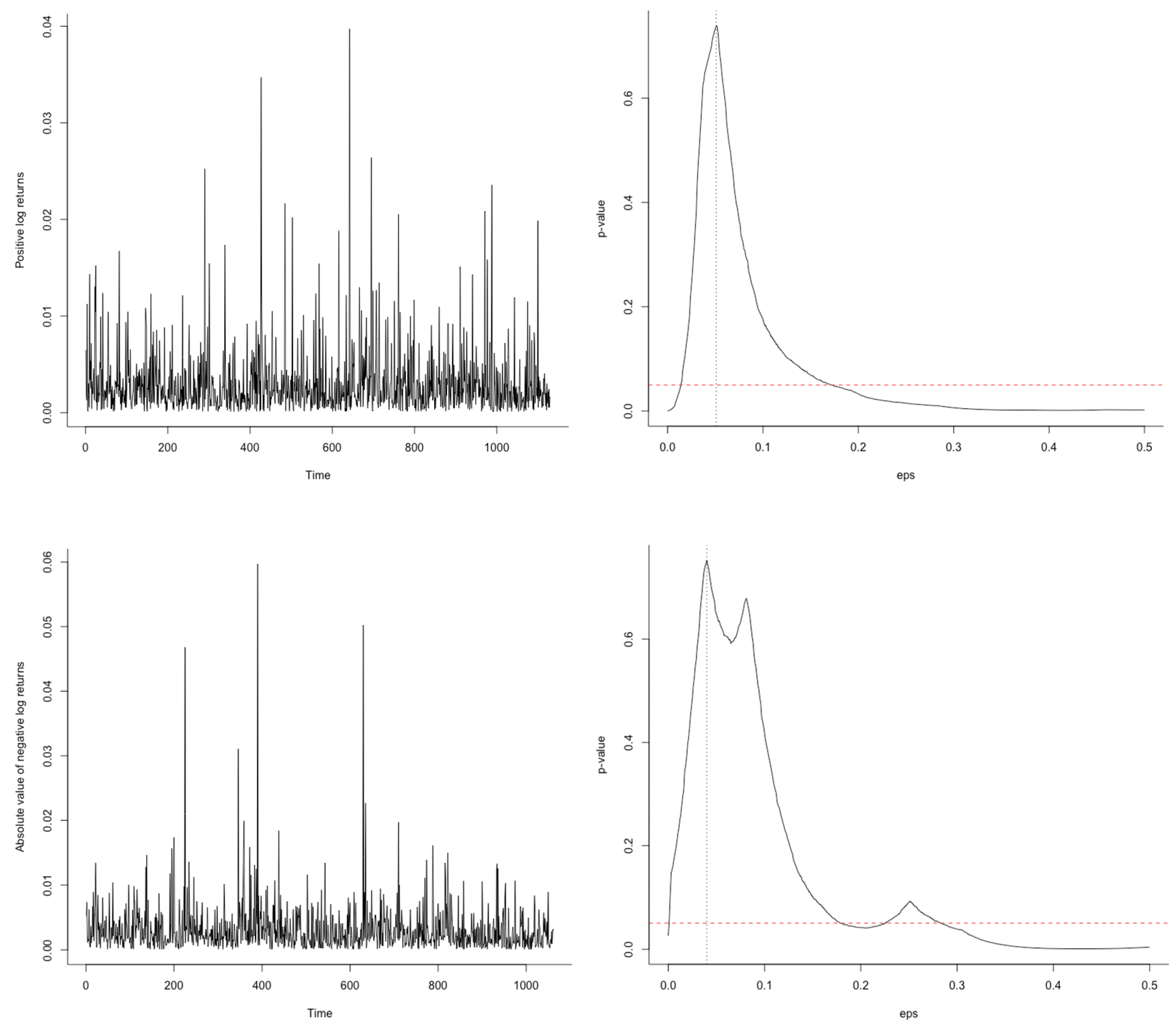
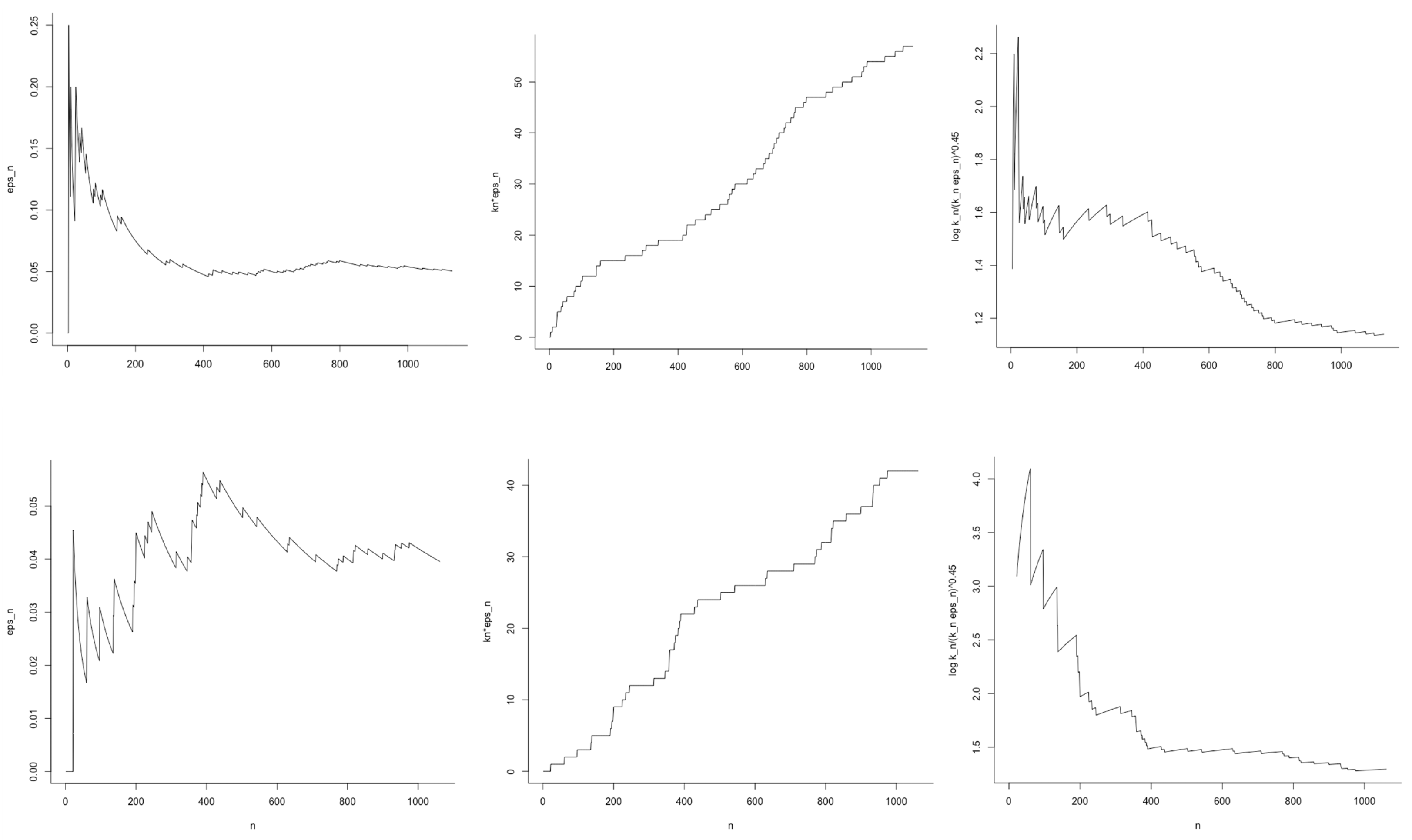
Starting from the prominent paper by Mandelbrot [18], heavy-tailedness of distributions of price changes is a well-known stylised fact, leading to the frequent choice of power laws for the modelling, see, e.g., [19]. However, numerous papers admit that the tails of the distributions used for modelling the returns are though heavier than normal, yet lighter than of a power law. For instance, Laherrère and Sornette [10] demonstrate that daily price variations on the exchange market can be successfully described by the Weibull distribution with parameter smaller than one. Malevergne et al. [11] intently analyse financial returns on different time scales, ranging from daily to 5- and 1-minute data, and come to the conclusion that the Pareto distribution fits the highest 5% of the data, while the remaining 95% are most efficiently described by the Weibull law. Thus, it is reasonable to expect that the overall distribution of returns should be successfully described by the model which (in some sense) lies in between of these two distributions. This idea serves as a motivation of the application of the model (3) to modelling the log-returns.
In our study we consider hourly logarithmic returns of BMW shares in 2019. Following [11], we analyse positive and negative returns separately. The sample sizes are equal to 1130 and 1062, respectively. The plots for positive and negative log returns are presented in the first plot in Figure 3. In what follows, we assume that the log-returns are jointly independent. This assumption was checked by the chi-squared test resulting in p-values 0.234 and 0.111 for positive and negative returns, respectively.
The analysis consists of four steps. Below we denote the positive log-returns by X 1 , , X 1130 and the negative log-returns by Y 1 , , Y 1062 .
  • Separation of components. For each n = 1 , , 1130 , the sample X 1 , , X n is divided into two parts corresponding to the first and the second components in (14), where the slowly varying function L is equal to a constant. For such partition we assign all observations except the 1130 · ε 1130 greatest order statistics of the whole sample to the first component and test the goodness-of-fit for Weibull distribution by the Kolmogorov–Smirnov criterion. The values of ε 1130 are taken on a grid from 0 to 0.5 with a step of 0.001. From the second plot in Figure 3 it can be seen that there is an evident peak in p-values, which corresponds to some value of the mixture parameter, which we denote by ε ^ 1130 . The 1130 · ε ^ 1130 upper order statistics are assumed to come from the heavy-tailed part.
    Next, let us show that the sequence ε n vanishes as n grows. For all n = 1 , , 1129 the parameter ε n is estimated as the proportion of elements corresponding to the second component. The same procedure is applied for each n = 1 , , 1062 to the sample Y 1 , , Y n . The results are illustrated by Figure 4. The first plot in two rows indicates that in both cases ε ^ n declines with n, though in case of negative log returns the decrease is not so evident. From the second plot one can see that k n ε ^ n with k n = n appear to tend to infinity. Therefore, as suggested by Theorems 1 and 2, we examine the asymptotic behaviour of the ratio log k n / ( k n ε ^ n ) β for different values of β > 0 . For both positive and absolute values of negative log returns we get that for β = 0.45 this ratio decreases rapidly.
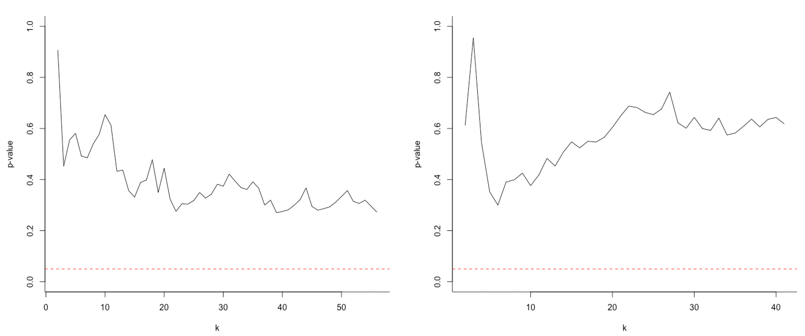
  • Model selection. Based on the partition obtained on the previous step, the decision between truncated and non-truncated distributions for the second component is made based on the test proposed by Aban, Meerschaert and Panorska [20]. From Figure 5 one observes that the null hypothesis of non-truncated law is not rejected for both positive and negative log returns since the p-values are significantly larger than 0.05. Thus, it can be concluded that the model (3) is more appropriate for the considered data. The Kolmogorov–Smirnov test does not reject the null of Pareto distribution for the observations assigned to the second component with p-values 0.971 and 0.925 for positive and negative log returns, respectively. It should be noted that in both cases the Pareto distribution does not fit the whole sample, since the p-values are smaller than 10 16 .
  • Estimation of parameters. The parameters of the first and second components are estimated by the maximum-likelihood approach. The estimated values are presented in Table 3. Since τ ^ / α ^ is equal to 0.483 for positive log returns and 0.484 for absolute values of negative, from Figure 4 we conclude that the assumption (9) is fulfilled with β = 0.45 , and therefore the limit distribution for maxima is the Fréchet distribution, see item 2 in Theorem 1.
    It is worth mentioning that for both positive and absolute values of negative log returns we get α ^ > 2 , which is completely coherent with general empirical results for financial returns and addresses the common critique against models with infinite variance, see [19].
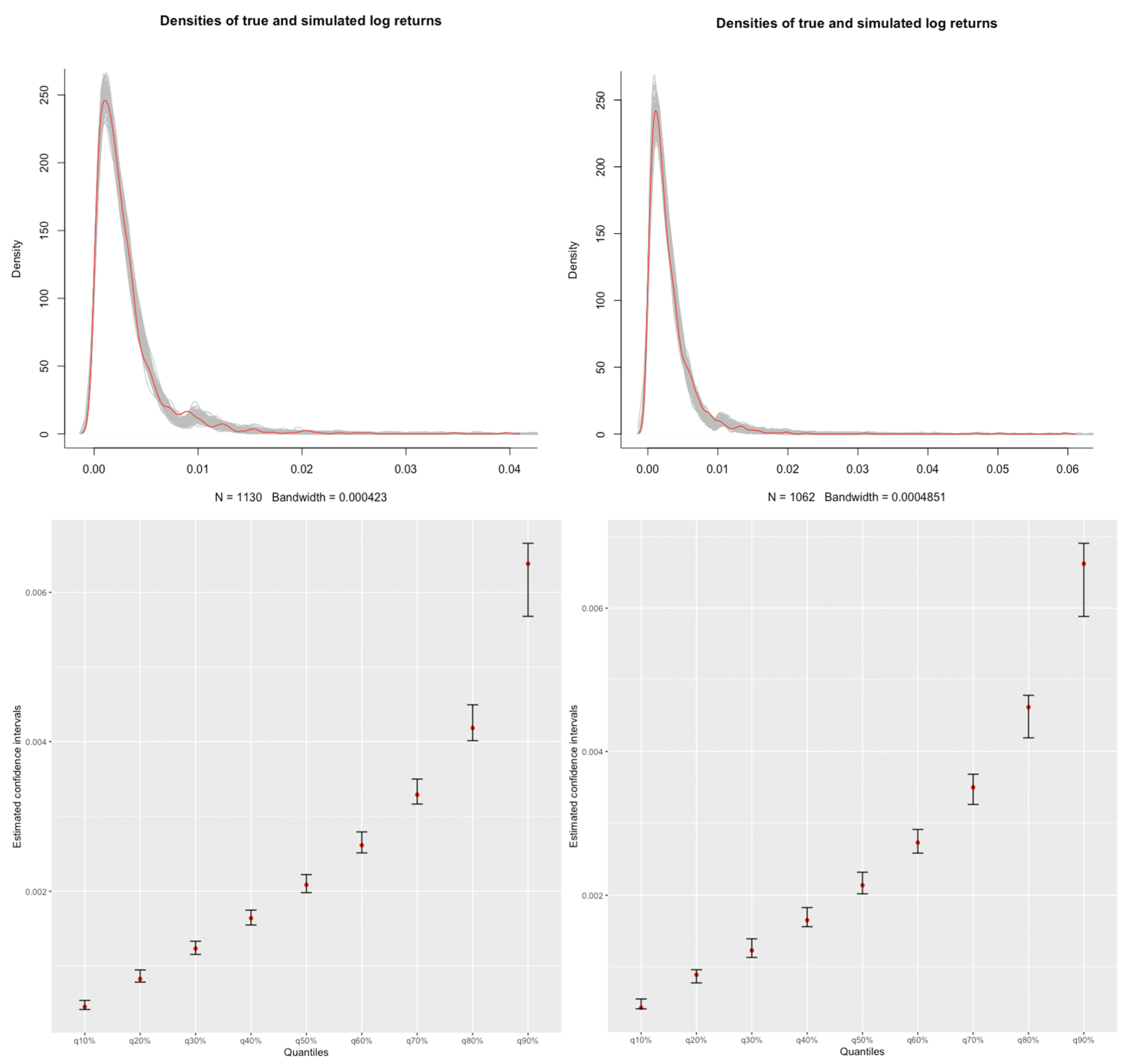
  • Validation of the model.Figure 6 depicts the true density of positive (top left) and absolute values of negative (top right) log returns superimposed with densities of 100 simulations from the mixture (3) with the corresponding parameter estimates. The constructed model is also verified by the empirical confidence intervals for the sample quantiles based on 100 simulations. The results are given in Table 4 and Table 5 and illustrated by Figure 6. These intervals are reasonably small and contain all true values of quantiles. Next, we apply the chi-squared test with the maximum likelihood estimates of parameters. Due to the known theory (see Section 4.4 from [21]), the statistics of this test converge to the chi-squared distribution with K 1 D degrees of freedom, where K is the number of subintervals used for the chi-squared test, and D is the dimension of the parameter space (in our setting, D = 5 ). Using K = 15 , we get the p-values 0.73 and 0.21 for positive and negative log returns, and therefore do not reject the null hypothesis. Finally, we arrive at the outcome that the model (3) is appropriate both for positive and absolute values of negative log returns of BMW at the considered time scale.

6. Conclusions

This paper contributes to the existing literature in the following respects.
  • We model the heavy-tailed impurity via the mixture distribution with varying parameters and (following the ideas from [8,9]) consider the resulting model as a triangular array. The notion of heavy-tailed impurity is not new, but all previously known probabilistic results are concentrated only on the classical limit laws, see [2,16]. In this paper, we establish the limit laws for the maximum in these models.
  • The paper delivers an example of the triangular array such that its row-wise maximum has (under proper normalisation) 6 different distributions, depending on the rates of the varying parameters. To the best of our knowledge, all previous articles on the extreme value analysis for triangular arrays deal with the convergence to the limit law having twice differentiable cdf ([5,7]) or closely related to the classical extreme value distributions ([6]), while some limits in our examples are discontinuous and very different from the classical laws.
  • We show the difference between various types of truncation for the regularly varying distributions used for modelling the impurity. Our conditions (17)–(18) are close to soft and hard truncation regimes introduced in [9], leading to similar (but not completely the same) outcomes for our mixture model as for the model considered in [9]. Moreover, unlike previous papers, we study in details the case of intermediate truncation regime (19).
  • For practical purposes we describe the four-step scheme for the application of this model to the asset price modelling. This approach can be considered as a possible development of the idea that the distribution of stock returns is in some sense between exponential and power law. A comprehensive discussion of this idea can be found in [11].

Author Contributions

Methodology, E.M. and V.P.; Supervision, V.P.; Visualization, E.M.; Writing—original draft, E.M.; Writing—review & editing, V.P. All authors have read and agreed to the published version of the manuscript.

Funding

The article was prepared in the framework of a research grant funded by the Ministry of Science and Higher Education of the Russian Federation (grant ID: 075-15-2020-928).

Institutional Review Board Statement

Not applicable.

Informed Consent Statement

Not applicable.

Data Availability Statement

Not applicable.

Conflicts of Interest

The authors declare no conflict of interest.

Appendix A. Classical EVA for the Mixture Model

Let us analyse the asymptotic behaviour of maxima of a sequence of i.i.d. random variables X 1 , X 2 , , X n , n 2 , with cumulative distribution function (3). That is, we consider
lim n P max i = 1 , , n X i v n ( x ) ,
where v n ( x ) = s n x + c n is some non-decreasing normalising sequence unbounded in n and x. Since X i , i = 1 , , n are independent,
lim n P max i = 1 , , n X i v n ( x ) = lim n P X 1 v n ( x ) n = lim n ( 1 ε ) ( 1 e λ v n τ ( x ) ) + ε ( 1 v n α ( x ) L ( v n ( x ) ) ) n = exp lim n n ( 1 ε ) e λ v n τ ( x ) + ε v n α ( x ) L ( v n ( x ) ) = exp lim n n ε v n α ( x ) L ( v n ( x ) ) × 1 ε ε · v n α ( x ) e λ ( v n ( x ) ) τ L ( v n ( x ) ) + 1 .
Since v n ( x ) as n , lim n v n α ( x ) e λ ( v n ( x ) ) τ L ( v n ( x ) ) 1 = 0 , and therefore
lim n P max i = 1 , , n X i v n ( x ) = exp lim n n ε v n α ( x ) L ( v n ( x ) ) .
Thus, the limit distribution for maxima is determined by the second component, leading to the Fréchet limit. In fact, choosing
c n = 0 , s n = ( 1 / F 2 ¯ ) ( n ) ,
we get
lim n P max i = 1 , , n X i v n ( x ) = exp ε x α ,
that is the Fréchet-type distribution.

Appendix B. Proof of Theorem 1

For given sequences s n , c n , the left-hand side of (11) can be represented as
lim n P X 1 v n ( x ) k n = lim n 1 ε n 1 e λ v n τ ( x ) + ε n 1 v n α ( x ) L ( v n ( x ) ) k n = lim n ( 1 e λ v n τ ( x ) ε n v n α ( x ) L ( v n ( x ) ) ) k n = exp lim n k n e λ v n τ ( x ) + k n ε n v n α ( x ) L ( v n ( x ) ) ,
where v n ( x ) = s n x + c n . Our aim is to find the sequences s n , c n guaranteeing that this limit (denoted by H ( x ) ) is non-degenerate. We divide the range of possible rates of convergence of k n , ε n into several essentially different cases.
(i)
Let k n ε n c [ 0 , ) . As v n α ( x ) L ( v n ( x ) ) 0 as n by the slow variation of L ( · ) (see (6)), we get
H ( x ) = exp lim n k n e λ v n τ ( x ) ,
and therefore we deal with the extreme value analysis of the Weibull law. Since F ¯ 1 ( x ) = e λ x τ , λ > 0 , τ 1 is a von Mises function, i.e., F ¯ 1 ( x ) can be represented as
F ¯ 1 ( x ) = c ˘ · exp 0 x 1 a ( u ) d u , 0 < x < ,
with c ˘ = 1 and a ( u ) = ( λ τ ) 1 u 1 τ , x > 0 , we get that the limit distribution is Gumbel under the choice v n ( x ) = s n x + c n with
c n : = F 1 1 1 k n = log k n λ 1 τ
s n : = a ( c n ) = ( λ τ ) 1 log k n λ 1 τ 1 .
(ii)
Let k n ε n as n . This case is divided into several subcases, depending on the relation between s n and c n .
  • First, let us consider s n | c n | . Then
    v n ( x ) = s n x + c n = s n x 1 + c n s n x = s n x ( 1 + o ¯ ( 1 ) )
    as n . Therefore,
    H ( x ) = exp lim n k n e λ s n τ x τ + k n ε n s n α x α L ( s n ) ,
    as L ( s n x ) L ( s n ) for all fixed x R as n . Clearly, since c n is not present in the above limit, one can take c n = 0 . As for s n , we have
    s n α L ( s n ) = 1 k n ε n ,
    i.e., s n : = F 2 1 ( k n ε n ) 1 . We have
    lim n k n e λ s n τ x τ = lim n exp s n τ λ x τ log k n s n τ ,
    and therefore the limit distribution in (A1) is non-degenerate (and is actually the Fréchet distribution) if and only if
    lim n log k n s n τ = 0 .
    It would be a worth mentioning that s n depends on the function L via the equality (A2). Let us recall that L ( · ) is slowly varying and therefore
    L ( s n ) s n ϵ ϵ > 0 .
    Thus, from (A2) we get
    1 k n ε n = s n α L ( s n ) s n α ϵ ϵ > 0 ,
    and
    s n ( k n ε n ) 1 ( α + ϵ ) ϵ > 0 .
    Now, since
    log k n s n τ log k n ( k n ε n ) τ ( α + ϵ ) ,
    we get that for the condition (A3) to be fulfilled, it is sufficient that the right-hand side tends to zero as n , i.e.,
    lim n log k n ( k n ε n ) τ ( α + ϵ ) = 0 ,
    or, equivalently,
    β ( 0 , τ α ) : lim n log k n ( k n ε n ) β = 0 .
    We conclude that the condition (A4) yields (A3), and in this case the limit distribution is Fréchet.
  • Now, let s n > 0 and c n R be such that s n | c n | . In this case
    v n ( x ) = s n x + c n = c n s n c n x + 1 = c n ( 1 + o ¯ ( 1 ) )
    as n . Thus, the limit in (A1) takes the form
    H ( x ) = exp lim n k n e λ ( s n x + c n ) τ + k n ε n c n α L ( c n ) .
    Let the norming constants c n and s n be chosen in the form (12). Then H ( x ) is the cdf of the Gumbel law if
    lim n k n ε n L ( log k n ) 1 τ ( log k n ) α τ = 0 .
    As previously, we would like to replace (A5) with another condition without L ( · ) . Once more, we would like to recall that by slow variation of L ( · )
    L ( x ) x ϵ ϵ > 0 .
    From this we conclude that
    k n ε n L ( log k n ) 1 τ ( log k n ) α τ k n ε n ( log k n ) ( α ϵ ) τ
    and the fact that the right-hand side tends to zero as n will imply (A5). In other words, we obtain the Gumbel limit if
    lim n k n ε n ( log k n ) ( α ϵ ) τ = lim n ( k n ε n ) τ ( α ϵ ) log k n ( α ϵ ) τ = 0 ,
    or, equivalently, if
    β > τ α : lim n log k n ( k n ε n ) β = .
  • The last possible situation is when neither (A4), nor (A6) is satisfied. Clearly, this is the case only when k n ε n c · ( log k n ) α τ for some c > 0 . Not surprisingly, it turns out that the final answer now depends on the asymptotic behaviour of L ( · ) .
(a)
Let us first consider L ( · ) the case L ( u ) as u . Then one can take c n = 0 and find s n as the solution to the equation
s n α L ( s n ) = 1 k n ε n 1 c · ( log k n ) α τ .
The limit for the second component in (A1) coincides with the corresponding one in item 2(i) (and leads to the cdf of the Fréchet law), while for the first component we get
lim n k n e λ s n τ x τ = lim n k n exp λ s n α L ( s n ) L ( s n ) τ α x τ = lim n k n 1 λ ( c L ( s n ) ) τ α x τ .
The value of the latter limit is zero for all fixed x > 0 since L ( s n ) as n , and therefore the limit distribution is Fréchet.
(b)
Now, let L ( · ) be such that L ( u ) c ˜ > 0 as u . Then the same choice of norming constants as when L ( u ) as u leads to the same limits as before. However, the value of (A7) now depends on x, namely,
lim n k n 1 λ ( c L ( s n ) ) τ α x τ = , x ( 0 , λ 1 τ ( c c ˜ ) 1 α ) , 1 , x = λ 1 τ ( c c ˜ ) 1 α , 0 , x > λ 1 τ ( c c ˜ ) 1 α .
Thus, in this case the limit distribution is equal to
lim n P max j = 1 , , k n X n j v n ( x ) = 0 , x < λ 1 τ ( c c ˜ ) 1 α , e ( 1 + x α ) , x = λ 1 τ ( c c ˜ ) 1 α , e x α , x > λ 1 τ ( c c ˜ ) 1 α .
An interesting point is that we get the limit distribution that is not from the extreme value family, having an atom at x = λ 1 τ ( c c ˜ ) 1 α .
(c)
Finally, let L ( · ) be such that L ( u ) 0 as u . Then the normalising sequence can be chosen as in item 1, and for the first component we get
lim n k n e λ v n τ ( x ) = e x x R ,
while for the second one
lim n k n ε n L ( c n ) c n α = lim n c · ( log k n ) α τ L ( log k n ) 1 τ ( log k n ) α τ = lim n c · L ( log k n ) 1 τ = 0 .
Therefore, in this case the limit distribution is again Gumbel.

Appendix C. Limit Law for the Truncated RV Distribution

Lemma A1. 
Let F ˜ 2 ( x ; α , M ) be the upper-truncated regularly varying distribution defined as (15). Then F ˜ 2 is in the maximum domain of attraction of the max-Weibull law Ψ τ having the distribution function
Ψ τ = e ( x ) τ I { x 0 } + I { x > 0 }
with τ = 1 .
Proof. 
As it is known, F M D A ( Ψ τ ) for some τ > 0 if and only if x * = sup x R : F ( x ) < 1 < and F ¯ x * 1 x R V τ , see, e.g., [15]. Thus, F ˜ 2 M D A ( Ψ τ ) for some τ > 0 if and only if
F ˜ ¯ 2 M 1 x = x τ L ˜ ( x ) , τ > 0 ,
for some slowly varying function L ˜ ( · ) , or, equivalently, iff
G ( x ) : = x τ F ˜ ¯ 2 M 1 x R V 0 , τ > 0 .
Therefore, to prove this statement of this lemma, we need to show that lim x ( G ( t x ) / G ( x ) ) = 1 for any t > 0 , that is,
lim x G ( t x ) G ( x ) = lim x t τ F ˜ ¯ 2 M 1 t x F ˜ ¯ 2 M 1 x        = lim x t τ M 1 t x α L M 1 t x M α L ( M ) M 1 x α L M 1 x M α L ( M ) = 1 t > 0 .
First,
lim x M 1 x α = lim x M α 1 1 M x α = M α + α M α 1 · 1 x ( 1 + o ¯ ( 1 ) ) .
Then, assuming that L ( · ) is continuous and differentiable,
lim x L M 1 x = L ( M ) L ( M ) · 1 x ( 1 + o ¯ ( 1 ) ) .
Therefore,
lim x t τ M 1 t x α L M 1 t x M α L ( M ) M 1 x α L M 1 x M α L ( M )      = lim x t τ M α + α M α 1 t x ( 1 + o ¯ ( 1 ) ) L ( M ) L ( M ) t x ( 1 + o ¯ ( 1 ) ) M α L ( M ) M α + α M α 1 x ( 1 + o ¯ ( 1 ) ) L ( M ) L ( M ) x ( 1 + o ¯ ( 1 ) ) M α L ( M ) = lim x t τ M α L ( M ) t x + α M α 1 t x L ( M ) ( 1 + o ¯ ( 1 ) ) M α L ( M ) x + α M α 1 x L ( M ) ( 1 + o ¯ ( 1 ) ) .
Clearly, the latter limit is equal to one if τ = 1 , meaning that F ˜ 2 M D A ( Ψ 1 ) . □

Appendix D. Proof of Theorem 2

Step 1. Several simple cases. As in the proof of Theorem 1, we use the notation v n ( x ) = s n x + c n . We have
H ( x ) = lim n ( ( 1 ε n ) ( 1 e λ v n τ ( x ) ) + ε n 1 v n α ( x ) L ( v n ( x ) ) 1 M n α L ( M n ) I { v n ( x ) [ m , M n ] } + I { v n ( x ) > M n } ) k n = lim n ( 1 ( 1 ε n ) e λ v n τ ( x ) + ε n M n α L ( M n ) v n α ( x ) L ( v n ( x ) ) 1 M n α L ( M n ) I { v n ( x ) [ m , M n ] } I { v n ( x ) < m } ) k n ,
where we use that I { v n ( x ) > M n } = 1 I { v n ( x ) [ m , M n ] } I { v n ( x ) < m } . Since ε n 0 , M n and M n α L ( M n ) 0 as n by slow variation of L ( · ) , we get
H ( x ) = lim n 1 e λ v n τ ( x ) + ε n ( ( M n α L ( M n ) v n α ( x ) L ( v n ( x ) ) ) I { v n ( x ) [ m , M n ] } I { v n ( x ) < m } ) k n = exp { lim n ( k n e λ v n τ ( x ) k n ε n ( M n α L ( M n ) v n α ( x ) L ( v n ( x ) ) ) I { v n ( x ) [ m , M n ] } + k n ε n I { v n ( x ) < m } ) } .
(i)
Let k n ε n 0 as n . By slow variation of L ( · ) , v n α ( x ) L ( v n ( x ) ) 0 as n , therefore, the whole second component disappears. We deal with maxima of a Weibull random variable and obtain the Gumbel limit under the normalisation v n ( x ) = s n x + c n with s n , c n in the form (A3).
(ii)
Let k n ε n = c o n s t . By a similar argument as in the previous item,
H ( x ) = lim n 1 1 k n [ k n e λ v n τ ( x ) + k n ε n I { v n ( x ) < m } ] k n .
Under the same choice of normalising sequences, we get
v n ( x ) = x λ τ log k n λ 1 τ 1 + log k n λ 1 τ = log k n λ 1 τ x τ log k n + 1
for all fixed x R as n . Therefore, the limit distribution is again Gumbel.
(iii)
Let k n ε n as n . The further analysis depends on the asymptotic properties of M n . If (17) holds, the proof is based on the observation that
M n α L ( M n ) M n α + ϵ ϵ > 0 ,
and therefore,
k n ε n M n α L ( M n ) k n ε n M n α + ϵ ϵ > 0 .
From (17) it follow that for any ϵ ( 0 , α 1 γ ] the right-hand side tends to zero as n , and therefore k n ε n M n α L ( M n ) 0 as n . The rest of the proof in this situation follows the same lines as the proof of Theorem 1. Other cases are more complicated, and we divide the further proof into several steps.
Step 2. Case (18). Recalling again that L ( · ) R V 0 , we get that
k n ε n M n α L ( M n ) k n ε n M n α ϵ ϵ > 0 .
Therefore, for any ϵ ( 0 , 1 γ α ] , k n ε n M n α L ( M n ) as n . Now, assume that v n ( x ) is such that v n ( x ) M n for all x R and n large enough. Then
lim x H ( x ) = exp { lim n lim x ( k n e λ v n τ ( x ) k n ε n ( M n α L ( M n ) v n α ( x ) L ( v n ( x ) ) ) I { v n ( x ) [ m , M n ] } + k n ε n I { v n ( x ) < m } ) } = e lim n k n ε n M n α L ( M n ) = ,
and therefore the limit distribution does not exist. We conclude that there is a non-degenerate limit distribution only if v n ( x ) > M n for all x R and n large enough. In this case,
k n e λ v n τ ( x ) = log ( H ( x ) ) ( 1 + o ¯ ( 1 ) ) .
The condition v n ( x ) > M n leads to the inequality
k n e λ M n τ > log ( H ( x ) ) ( 1 + o ¯ ( 1 ) )
for n sufficiently large. Finally, as log ( H ( x ) ) takes only non-negative values, and the sequences k n , M n tend to infinity as n , we conclude that the necessary condition for the existence of non-degenerate limit distribution is
M n τ log k n .
  • Now let us consider the case when (8) holds. We have
    M n τ log k n M n τ ( k n ε n ) β M n ( k n ε n ) γ τ ,
    since β > τ α > τ γ . The right-hand side tends to zero as n and therefore (A10) holds. Choosing s n and c n as in (12), we get that v n ( x ) > M n for all x R , and therefore the limit distribution is Gumbel.
  • Now assume that (9) holds. In this case, (A10) can be violated. In fact,
    M n τ log k n = M n ( log k n ) 1 τ τ ( k n ε n ) γ ( log k n ) 1 τ τ = ( k n ε n ) τ γ log k n
    with some γ ( 0 , 1 α ) . From (18), it follows that the right-hand side is infinite if τ γ β , and has an unknown asymptotic behaviour otherwise. The lower bound is given by
    M n τ log k n M n τ ( k n ε n ) β = M n ( k n ε n ) β τ τ ,
    where for β τ γ , the right-hand side tends to zero as n , while otherwise the asymptotic behaviour is again unknown. In this case, we conclude that if M n is such that (A10) holds, the non-degenerate limit distribution exists and is in fact the Gumbel distribution.
  • Finally, in the case (10),
    M n τ log k n c 1 α M n ( k n ε n ) 1 α τ c 1 α M n ( k n ε n ) γ τ ,
    because γ ( 0 , 1 α ) . Since by (A10) there exists γ ( 0 , 1 α ) such that the right-hand side tends to zero as n , we get under proper normalisation the Gumbel limit distribution.
Step 3. Case (19).
  • If (8) is satisfied, it is possible to obtain the Gumbel limit under the same choice of normalising sequence (12). Indeed, in this case
    M n τ log k n c ˘ τ ( k n ε n ) τ α log k n ( k n ε n ) β log k n ,
    because β > τ α . Therefore, (A10) follows from (8), and we obtain the Gumbel distribution as a limit.
  • If (9) holds, then the result turns out to depend on the asymptotic behaviour of L ( · ) . Let us recall that k n ε n M n α is asymptotically equal to a constant.
    (a)
    If L ( u ) as u , we have that k n ε n M n α L ( M n ) as n . Thus, as was argued above, the non-degerated limit H ( x ) exists if and only if (A10) holds for all x and n large enough. However, for any β ( 0 , τ α ) ,
    M n τ log k n c ˘ τ ( k n ε n ) τ α log k n ( k n ε n ) β log k n ,
    and therefore the assumption (A10) is violated due to (9). Thus, in this case there exists no non-degenerate limit distribution.
    (b)
    Now consider the case L ( u ) c ˜ for some c ˜ > 0 as u . Let us fix s n , c n in the form (13). The inequality v n ( x ) = s n x > M n is equivalent to x > c ˘ c ˜ 1 α . Under this normalisation, we have
    lim n k n e λ v n τ ( x ) = 0 ,
    and therefore
    H ( x ) = e c ˜ c ˘ α x α , x ( 0 , c ˘ c ˜ 1 α ] , 1 , x > c ˘ c ˜ 1 α .
    (c)
    If L ( u ) 0 as u , one can take the norming constants as in the previous item and obtain the Fréchet limit distribution since k n ε n M n α L ( M n ) 0 and k n ε n s n α L ( s n ) x α x α as n . The last thing which is crucial here is to check that v n ( x ) M n for all x R . This inequality follows from
    s n x = ( k n ε n ) 1 α L 1 α ( s n ) x c ˘ 1 M n L 1 α ( s n ) x M n .
  • Finally, let us consider the case (10). As in the previous situations, the limit distribution depends on the asymptotic behaviour of L ( · ) .
    (a)
    Let L ( u ) as u . Since then k n ε n M n α L ( M n ) as n , we conclude that the non-degenerate limit exists only if (A9) holds. In the considered case, (A9) is equivalent to
    λ 1 / τ c ˘ c 1 / α < 1
    The normalising sequence (12) again leads to the Gumbel limit distribution.
    (b)
    If L ( u ) c ˜ for some c ˜ > 0 as u , we have that k n ε n M n α L ( M n ) c ˜ c ˘ α .
    • If λ 1 τ c ˘ c 1 α < 1 , a linear normalising sequence as in (12) leads to the Gumbel limit, since v n ( x ) > M n for all x R and n large enough; see the previous item.
    • If λ 1 τ c ˘ c 1 α > 1 , the choice (13) of normalising constants yields s n x > M n for all x > c ˘ c ˜ 1 α , while
      lim n k n e λ s n τ x τ = k n 1 ( c c ˜ ) τ α x τ = , x ( 0 , λ 1 τ ( c c ˜ ) 1 α ) , 1 , x = λ 1 τ ( c c ˜ ) 1 α , 0 , x > λ 1 τ ( c c ˜ ) 1 α
      and
      lim n k n ε n s n α L ( s n ) x α = x α .
      Therefore, we get
      H ( x ) = 0 , x ( 0 , λ 1 τ ( c c ˜ ) 1 α ) , exp 1 + c ˜ c ˘ α λ α τ c c ˜ , x = λ 1 τ ( c c ˜ ) 1 α , exp c ˜ c ˘ α x α , x ( λ 1 τ ( c c ˜ ) 1 α , c ˘ c ˜ 1 α ] , 1 , x > c ˘ c ˜ 1 α .
      As we see, the limit distribution does not belong to the extreme value family, and has an atom at x = λ 1 τ ( c c ˜ ) 1 α .
    • If λ 1 τ c ˘ c 1 α = 1 , the choice (13) leads to the discrete limit distribution having a unique atom at x = c ˘ c ˜ 1 α with probability mass 1 / e .
    (c)
    Lastly, let L ( · ) be such that L ( u ) 0 as u . Then the Gumbel limit can be obtained under the normalisation (12) since k n ε n M n α L ( M n ) 0 as n , see item (i,c) in Theorem 1. This observation completes the proof.

References

  1. van den Berg, J.; Nolin, P. Near-critical percolation with heavy-tailed impurities, forest fires and frozen percolation. arXiv 2018, arXiv:1810.08181. [Google Scholar]
  2. Grabchak, M.; Molchanov, S. Limit theorems and phase transitions for two models of summation of independent identically distributed random variables with a parameter. Theory Prob. Appl. 2015, 59, 222–243. [Google Scholar] [CrossRef]
  3. Petrov, V. Sums of Independent Random Variables; Springer Science & Business Media: Norwell, MA, USA, 2012; Volume 82. [Google Scholar]
  4. Meerschaert, M.; Scheffler, H.-P. Limit Distributions for Sums of Independent Random Vectors: Heavy Tails in Theory and Practice; John Wiley & Sons: New York, NY, USA, 2001; Volume 321. [Google Scholar]
  5. Freitas, A.; Hüsler, J. Condition for the convergence of maxima of random triangular arrays. Extremes 2003, 6, 381–394. [Google Scholar] [CrossRef]
  6. Anderson, C.; Coles, S.; Hüsler, J. Maxima of Poisson-like variables and related triangular arrays. Ann. Appl. Probab. 1997, 7, 953–971. [Google Scholar] [CrossRef]
  7. Dkengne, P.S.; Eckert, N.; Naveau, P. A limiting distribution for maxima of discrete stationary triangular arrays with an application to risk due to avalanches. Extremes 2016, 19, 25–40. [Google Scholar] [CrossRef]
  8. Beirlant, J.; Fraga, A.I.; Gomes, I. Tail fitting for truncated and non-truncated Pareto-type distributions. Extremes 2016, 19, 429–462. [Google Scholar] [CrossRef] [Green Version]
  9. Chakrabarty, A.; Samorodnitsky, G. Understanding heavy tails in a bounded world or, is a truncated heavy tail heavy or not? Stoch. Model. 2012, 28, 109–143. [Google Scholar] [CrossRef] [Green Version]
  10. Laherrere, J.; Sornette, D. Stretched exponential distributions in nature and economy: “Fat tails” with characteristic scales. Eur. Phys. J. -Condens. Matter Complex Syst. 1998, 2, 525–539. [Google Scholar] [CrossRef] [Green Version]
  11. Malevergne, Y.; Pisarenko, V.; Sornette, D. Empirical distributions of stock returns: Between the stretched exponential and the power law? Quant. Financ. 2005, 5, 379–401. [Google Scholar] [CrossRef]
  12. Bingham, N.H.; Goldie, C.M.; Teugels, J.L. Regular Variation; Cambridge University Press: Cambridge, UK, 1987. [Google Scholar]
  13. Resnick, S. Extreme Values, Regular Variation and Point Processes; Springer: New York, NY, USA, 2013. [Google Scholar]
  14. Mikosch, T. Regular Variation, Subexponentiality and Their Applications in Probability Theory; Report Eurandom; Eurandom: Eindhoven, The Netherlands, 1999; Volume 99013. [Google Scholar]
  15. Embrechts, P.; Klüppelberg, C.; Mikosch, T. Modelling Extremal Events for Insurance and Finance; Springer: New York, NY, USA, 1997. [Google Scholar]
  16. Panov, V. Limit theorems for sums of random variables with mixture distribution. Stat. Probab. Lett. 2017, 129, 379–386. [Google Scholar] [CrossRef] [Green Version]
  17. Paulauskas, V. A note on linear processes with tapered innovations. Lith. Math. J. 2020, 60, 64–79. [Google Scholar] [CrossRef] [Green Version]
  18. Mandelbrot, B. The variation of certain speculative prices. J. Bus. 1963, 1, 223. [Google Scholar] [CrossRef]
  19. Cont, R. Empirical properties of asset returns: Stylized facts and statistical issues. Quant. Financ. 2001, 1, 223–236. [Google Scholar] [CrossRef]
  20. Aban, I.B.; Meerschaert, M.M.; Panorska, A.K. Parameter estimation for the truncated Pareto distribution. J. Am. Stat. Assoc. 2006, 101, 270–277. [Google Scholar] [CrossRef]
  21. Suhov, Y.; Kelbert, M. Probability and Statistics by Example: Volume I. Basic Probability and Statistics; Cambridge University Press: Cambridge, UK, 2005. [Google Scholar]
Figure 1. Possible limit distributions for maxima of the triangular array (3).
Mathematics 09 02208 g001
Figure 2. Densities of sample maxima for groups (8)–(17) (top left), (9)–(17) (top right), (8)–(18) (bottom left) and (9)–(18) (bottom right) superimposed with the theoretical limit distributions suggested by Theorem 2.
Mathematics 09 02208 g002
Figure 3. First (second) row: The plot of data; p-values for Weibull fit for positive (absolute negative) log returns.
Mathematics 09 02208 g003
Figure 4. ε ^ n against n (left), k n ε ^ n against n (middle), log k n ( k n ε ^ n ) 0.45 against n (right) for positive log returns of BMW (first row) and absolute values of negative log returns of BMW (second row).
Mathematics 09 02208 g004
Figure 5. The p-values of the Aban’s test for positive (left) and absolute values of negative (right) log returns.
Mathematics 09 02208 g005
Figure 6. Top left (right): Real (red) and simulated (grey) density of positive (negative) log returns; bottom left (right): Empirical quantiles of positive (negative) log returns and the corresponding confidence intervals.
Mathematics 09 02208 g006
Table 1. Possible limit distributions for maxima of the triangular array (16).
k n ε n n (8)(9)(10)
(17)GumbelFréchetGumbel,
if L ( u ) u 0
Fréchet,
if L ( u ) u
Distribution I,
if L ( u ) u c ˜ ( 0 , )
(18)GumbelGumbel,Gumbel
if k n e λ M n τ
no limit,
if k n e λ M n τ is not fulfilled
(19)GumbelFréchet,Gumbel,
if L ( u ) u 0
if L ( u ) u 0 Gumbel,
if L ( u ) u c ˜ ( 0 , ] ,
and λ 1 τ c ˘ c 1 α ( 0 , 1 )
Distribution II,Distribution III,
if L ( u ) u c ˜ ( 0 , ) ,
and λ 1 τ c ˘ c 1 α > 1
if L ( u ) u c ˜ ( 0 , ) Distribution IV,
if L ( u ) u c ˜ ( 0 , ) ,
and λ 1 τ c ˘ c 1 α = 1
no limit,no limit,
if L ( u ) u if L ( u ) u ,
and λ 1 τ c ˘ c 1 α 1
Table 2. The values of ε n and M n chosen for the numerical study.
(8)(9)
(17) ε n = n 1 log n , ε n = n 1 ( log n ) 2 ,
M n = log ( n + 1 ) M n = ( log ( n + 1 ) ) 2
(18) ε n = n 1 log n , ε n = n 1 ( log n ) 2 ,
M n = log ( n + 1 ) M n = log ( n + 1 )
Table 3. Estimated values of the parameters of mixture distribution for positive and absolute values of negative log returns of BMW, 2019.
Estimates λ ^ τ ^ α ^ m ^ ε ^
Positive log returns0.0031.2782.6490.0090.051
Abs. negative log returns0.0031.2462.5730.010.04
Table 4. Empirical quantiles of positive log returns of BMW, 2019, and the estimated confidence intervals.
Quantiles · 10 3 10%20%30%40%50%60%70%80%90%
Lower CI0.4160.7831.1541.5481.9822.5093.1644.0135.679
Estimate0.4520.8251.2321.642.0852.6113.2894.1836.383
Upper CI0.5370.9461.331.7472.2232.793.4984.4936.657
Table 5. Empirical quantiles of absolute values of negative log returns of BMW, 2019, and the estimated confidence intervals.
Quantiles · 10 3 10%20%30%40%50%60%70%80%90%
Lower CI0.4170.7781.1341.5622.0212.5833.2624.1915.884
Estimate0.4310.8921.2311.6542.142.733.5014.6196.62
Upper CI0.5540.9621.3931.8292.3212.9143.6844.7846.905
Publisher’s Note: MDPI stays neutral with regard to jurisdictional claims in published maps and institutional affiliations.

