Coupled Discrete Fractional-Order Logistic Maps

Abstract

This paper studies a system of coupled discrete fractional-order logistic maps, modeled by Caputo’s delta fractional difference, regarding its numerical integration and chaotic dynamics. Some interesting new dynamical properties and unusual phenomena from this coupled chaotic-map system are revealed. Moreover, the coexistence of attractors, a necessary ingredient of the existence of hidden attractors, is proved and analyzed.

1. Introduction

Nonlinear phenomena are difficult to describe by models analysis based only on smoothness; thereby, fractional calculus has been used to model many such processes for which the standard integer-order derivatives cannot be applied adequately. The generalization of the concept of derivatives of non-integer values dates back to the beginning of the theory of differential calculus, while the rapid development of the theory of fractional calculus started from the work of Euler, Liouville, Riemann, Letnikov, and so on [1,2]. In the past, new results of fractional modeling and applications were reported every year. The fractional derivatives and integrals are useful in engineering and mathematics, being helpful for scientists and researchers working with real-life applications (see, e.g., [3,4]).

It is well-known that the classical derivative of a continuous-time periodic function is a periodic function with the same period. However, with respect to derivatives of fractional order, this is not necessarily the case [5,6,7,8,9,10,11,12]. The non-periodicity of solutions in fractional-order (FO) systems was first discovered by engineers (see, e.g., [7]), and then proved by mathematicians (see, e.g., [5,12]). Generally, FO systems have no non-constant periodic solutions by their nature (verified, e.g., using Laplace or Z transformations). Nevertheless, both continuous and discrete FO systems may have asymptotic periodic solutions. However, just like continuous FO systems, the periodicity of solutions in discrete FO systems is a delicate issue [10,13,14,15,16,17]. As a consequence, all reported results based on the “periodicity” of continuous- or discrete-time autonomous FO systems became questionable.

In this paper, orbits apparently indicating some regular behavior will be called “periodic-like” orbits. Recall that for some values of the bifurcation parameter of the integral-order (IO) logistic map, unstable periodic orbits (UPOs) will emerge, leading to chaos. For FO logistic maps, this will be referred to as “chaotic-like” behavior. In [18], these kinds of periodic-like orbits are called “numerically periodic orbits”. It is also well-known that in the theory of dynamical systems, every emerging abrupt period-doubling phenomenon is considered as bifurcation. Therefore, in this paper, the term bifurcation or bifurcation diagram is understood in the above sense of a periodic-like phenomenon.

On the other hand, from a computational point of view, based on the complexity or simplicity in finding a basin of attraction in the phase space, it is natural to consider the following classification of attractors: self-excited attractors, which can be revealed numerically by integrating the systems with initial conditions within small neighborhoods of unstable equilibria, and hidden attractors, which have the basins of attraction not connected with any equilibria [19,20,21,22,23]. Examples of hidden attractors in continuous-time FO systems exist in some classical systems, such as the Rabinovich-Fabrikant system [24,25,26], Hopfield neuronal system [27], economic system [28], hyperchaotic discontinuous system [29], and so on [30].

In a numerical approach, the need for previous history in numerical integration requires a trade-off between the calculation time and the approximation precision. This is a basic principle for some classical numerical methods for fractional differential equations (FDEs), such as the Adams-Bashforth-Moulton method [31], for which a tutorial can be found in [32]. Finally, it should also be noted that the mathematical theory of FDEs is still quite limited today, although the subject has been studied since 1956 [33].

With all the above motivations and background, the present paper is devoted to studying a system of discrete coupled FO logistic maps, with respect to its numerical bifurcation analysis and hidden attractor search, which reveals some very interesting new dynamical properties and unusual phenomena.

This paper will also discuss the stability of discrete FO equations, where [34,35,36] can be referred to for more details.

2. A Model of Coupled FO Logistic Maps

In [37], the bistability of some “aggregates” of logistic maps with excitation-type coupling is studied. One such model is composed by two functional units, a neuron or a group of neurons (voxels), as a discrete nonlinear oscillator with two possible states: active (meaning one type of activity) or not (meaning other type of activity). A reasonable modality to take the most elemental local nonlinearity is, for instance, the logistic evolution:

$$\begin{array}{c}x(n+1)=p\left(3y\right(n)+1)x\left(n\right)(1-x(n\left)\right),\hfill \\ y(n+1)=p(-3x(n)+4)y\left(n\right)(1-y(n\left)\right),n\in \mathbb{N}.\hfill \end{array}$$

(1)

The first equation with the coupled functional units (1) refers to excitation coupling, while the second equation, to inhibition coupling. These kinds of models are proposed in [37] to mimic the waking-sleeping bistability and even multistability found in brain systems (see [37] for details).

In this paper, the Fractional Order (FO) variant of the system (1) is considered.

To obtain the FO form, let $N_a=\{a,a+1,a+2,\dots \}$. Then, for $q>0$ and $q\notin \mathbb{N}$, the q-th Caputo-like discrete fractional difference of a function $u:N_a\to \mathbb{R}$ is defined as [38,39]

$${\Delta }_a^{q}u\left(t\right)={\Delta }_a^{-(n-q)}{\Delta }^{n}u\left(t\right)=\frac{1}{\Gamma (n-q)}\sum _{s=a}^{t-(n-q)}{(t-s-1)}^{(n-q-1)}{\Delta }^{n}u\left(s\right),$$

(2)

for $t\in N_{a+n-q}$ and $n=\left[q\right]+1$. In (4), ${\Delta }^n$ is the n-th order forward difference operator,

$${\Delta }^{n}u\left(s\right)=\sum _{k=0}^n\left(\genfrac{}{}{0pt}{}{n}{k}\right){(-1)}^{n-k}u(s+k)$$

and ${\Delta }_a^{-q}$ represents the fractional sum of order q of u, namely,

$${\Delta }_a^{-q}u\left(t\right)=\frac{1}{\Gamma \left(q\right)}\sum _{s=a}^{t-q}{(t-s-1)}^{(q-1)}u\left(s\right),t\in {\mathbb{N}}_{a+q}$$

(3)

with the falling factorial $t^{\left(q\right)}$ in the following form:

$$t^{\left(q\right)}=\frac{\Gamma (t+1)}{\Gamma (t-q+1)}.$$

Note that the fractional operator ${\Delta }_a^{-q}$ maps functions defined on ${\mathbb{N}}_a$ to functions on ${\mathbb{N}}_{a+q}$.

For the case considered in this paper, $q\in (0,1)$, when $n=1$, $\Delta u\left(s\right)=u(s+1)-u\left(s\right)$, and Caputo’s fractional difference, denoted hereafter ${\Delta }_{\ast }^q$, becomes

$${\Delta }_{\ast }^{q}u\left(t\right)=\frac{1}{\Gamma (1-q)}\sum _{s=a}^{t-(1-q)}{(t-s-1)}^{(-q)}\Delta u\left(s\right).$$

(4)

Assuming the starting point of the fractional sum (3), $a=0$, one can consider the following discrete autonomous Initial Value Problem (IVP) of FO (the non-autonomous case can be found in [40,41]):

$${\Delta }_{\ast }^{q}u\left(t\right)=f\left(u(t+q-1)\right),t\in N_{1-q},u\left(0\right)=u_0,$$

(5)

for $q\in (0,1)$ and f is a continuous map.

The solution of the IVP (5) is given by [40,41]

$$u\left(t\right)=u_0+\frac{1}{\Gamma \left(q\right)}\sum _{s=1-q}^{t-q}{(t-s-1)}^{(q-1)}f\left(u(s+q-1)\right).$$

(6)

A convenient iterative form of the integral (6) is [35]

$$u\left(n\right)=u\left(0\right)+\frac{1}{\Gamma \left(q\right)}\sum _{i=1}^n\frac{\Gamma (n-i+q)}{\Gamma (n-i+1)}f\left(u(i-1)\right),u\left(0\right)=u_0,n\in \mathbb{N},n>0.$$

(7)

Now, one can introduce the FO variant of the system (1) modeled by the Caputo delta fractional difference equation:

$$\begin{array}{c}{\Delta }_{\ast }^{q}x\left(t\right)=p(3y(t+q-1)+1)x(t+q-1)(1-x(t+q-1)),\hfill \\ {\Delta }_{\ast }^{q}y\left(t\right)=p(-3x(t+q-1)+4)y(t+q-1)(1-y(t+q-1)),\hfill \\ t\in {\mathbb{N}}_{1-q},x\left(0\right)=x_0,y\left(0\right)=y_0,\hfill \end{array}$$

(8)

where $p\in \mathbb{R}$ is a parameter. In this case,

$$f\left(u\right):=f(x,y)=\left(\begin{array}{c}p(3y+1)x(1-x)\hfill \\ p(-3x+4)y(1-y)\hfill \end{array}\right),$$

(9)

and the integral (7) has the following form, which will be used to integrate and simulate the system dynamics later:

$$\begin{array}{c}x\left(n\right)=x\left(0\right)+\frac{1}{\Gamma \left(q\right)}{\displaystyle \sum _{i=1}^n}\frac{\Gamma (n-i+q)}{\Gamma (n-i+1)}p(3y(i-1)+1)x(i-1)(1-x(i-1)),\hfill \\ y\left(n\right)=y\left(0\right)+\frac{1}{\Gamma \left(q\right)}{\displaystyle \sum _{i=1}^n}\frac{\Gamma (n-i+q)}{\Gamma (n-i+1)}p(-3x(i-1)+4)y(i-1)(1-y(i-1)),\hfill \\ n\in \mathbb{N},n>0,x\left(0\right)=x_0,y\left(0\right)=y_0.\hfill \end{array}$$

(10)

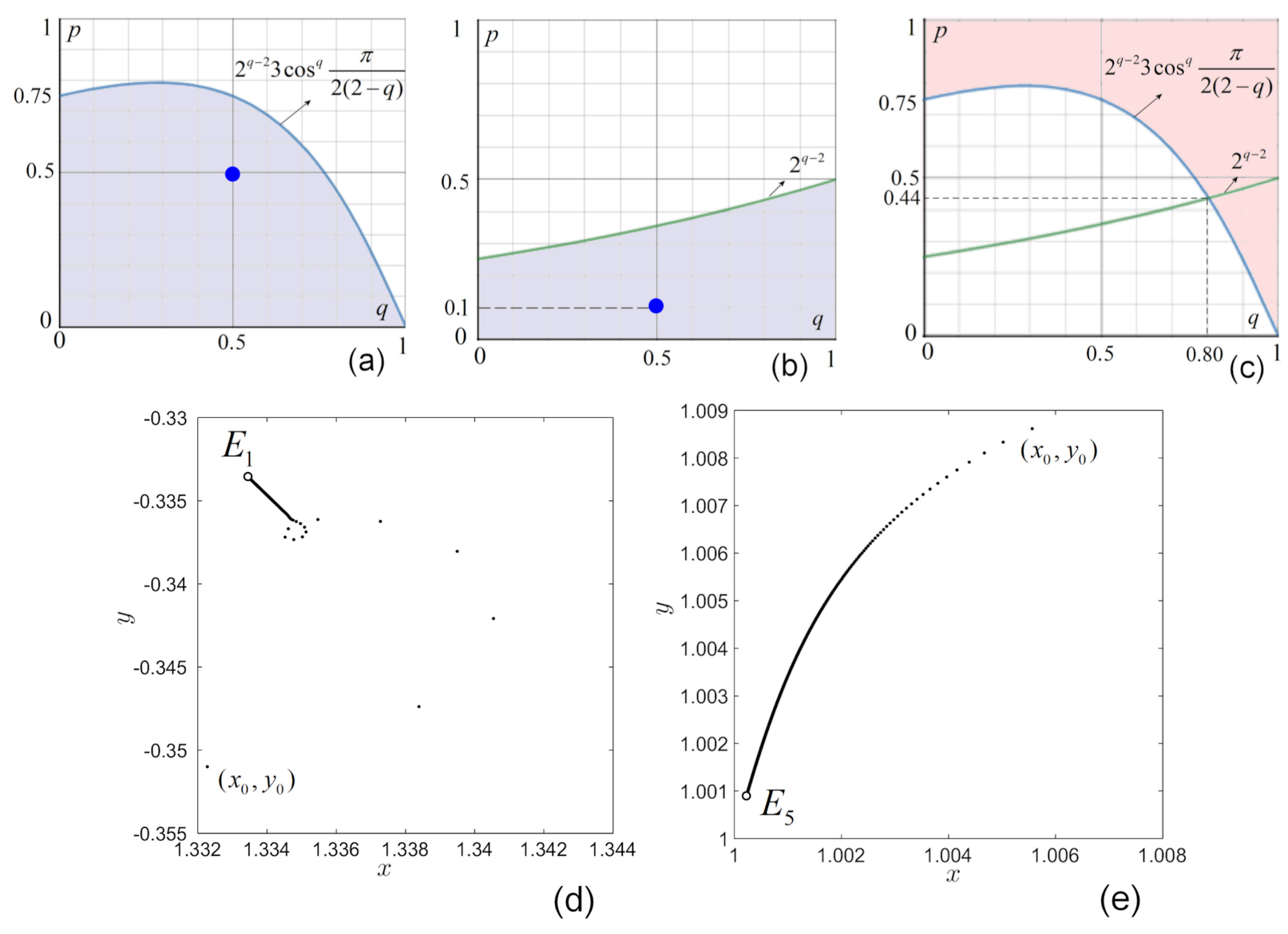
3. Bounds and Global Dynamics

The theory of orbits for discrete FO systems is technically rather sophisticated in general and is still under development. Additionally, finding either bounds of solutions or qualitative properties of global dynamics are difficult tasks.

Nevertheless, from the expressions (10), one can see that $x\left(n\right)$ and $y\left(n\right)$ are polynomials of p, that is,

$$\begin{array}{c}x\left(n\right)={\displaystyle \sum _{j=0}^{k\left(n\right)}}{a}_{nj}(x\left(0\right),y\left(0\right))p^j\\ y\left(n\right)={\displaystyle \sum _{j=0}^{k\left(n\right)}}{b}_{nj}(x\left(0\right),y\left(0\right))p^j,\end{array}$$

(11)

where the coefficients $a_{nj}(x\left(0\right),y\left(0\right))$, $b_{nj}(x\left(0\right),y\left(0\right))$ are polynomials of $x\left(0\right)$, $y\left(0\right)$.

From (10), the degree k of polynomials (11) is

$$k\left(0\right)=0,k\left(n\right)=3k(n-1)+1,n\ge 1,$$

so

$$k\left(n\right)=\frac{3^n-1}{2}.$$

The formulas $a_{nj}(x\left(0\right),y\left(0\right))$ and $b_{nj}(x\left(0\right),y\left(0\right))$ are difficult to find explicitly for general n, but nevertheless, one can find that

$$\begin{array}{c}{a}_{n0}(x\left(0\right),y\left(0\right))=x\left(0\right),b_{n0}(x\left(0\right),y\left(0\right))=y\left(0\right),\\ a_{n1}(x\left(0\right),y\left(0\right))=\frac{\left(3y\right(0)+1)x\left(0\right)(1-x(0\left)\right)}{\Gamma \left(q\right)}{\displaystyle \sum _{i=1}^n}\frac{\Gamma (n-i+q)}{\Gamma (n-i+1)},\\ b_{n1}(x\left(0\right),y\left(0\right))=\frac{(-3x(0)+4)y\left(0\right)(1-y(0\left)\right)}{\Gamma \left(q\right)}{\displaystyle \sum _{i=1}^n}\frac{\Gamma (n-i+q)}{\Gamma (n-i+1)}.\end{array}$$

Using [42] (Proposition 1), one obtains the following result.

Theorem 1.

The following limits hold:

$$\begin{array}{c}\underset{n\to \infty }{lim}\frac{a_{n1}(x\left(0\right),y\left(0\right))}{n^q}=\frac{\left(3y\right(0)+1)x\left(0\right)(1-x(0\left)\right)}{\Gamma (q+1)},\\ \underset{n\to \infty }{lim}\frac{b_{n1}(x\left(0\right),y\left(0\right))}{n^q}=\frac{(-3x(0)+4)y\left(0\right)(1-y(0\left)\right)}{\Gamma (q+1)}.\end{array}$$

Consequently, the first-order approximations of (11) diverges to ∞ as$n\to \infty$, except at the equilibria, where$f\left(u\right(0\left)\right)=0$.

Concerning global dynamics, the following result holds (for the dynamical behavior of discrete-time linear FO systems, see [43]).

Theorem 2.

There is no orbit ${\left\{(x\left(n\right),y\left(n\right))\right\}}_{n=1}^{\infty }$ of (8) such that

$$(x\left(n\right),y\left(n\right))\in S,\forall n\ge n_0,$$

(12)

for some $n_0\in \mathbb{N}$, where S is one of the following subsets of ${\mathbb{R}}^2$:

$$\begin{array}{c}\left\{x\ge 1+\delta ,y\ge -\frac{1}{3}+\delta \right\},\left\{x\le -\delta ,y\le -\frac{1}{3}-\delta \right\},\\ \left\{x\le \frac{4}{3}+\delta ,y\ge 1+\delta \right\},\left\{x\ge \frac{4}{3}+\delta ,y\le -\delta \right\},\end{array}$$

(13)

with$\delta >0$.

Proof.

(1)

If $S=\{x\ge 1+\delta ,y\ge -\frac{1}{3}+\delta \}$ and (12) holds, then (7) implies that

$$\begin{array}{ccc}\hfill x\left(n\right)& =& x\left(0\right)+\frac{p}{\Gamma \left(q\right)}\sum _{i=1}^{n_0}\frac{\Gamma (n-i+q)}{\Gamma (n-i+1)}(3y(i-1)+1)x(i-1)(1-x(i-1))\hfill \\ & & +\frac{p}{\Gamma \left(q\right)}\sum _{i=n_0+1}^n\frac{\Gamma (n-i+q)}{\Gamma (n-i+1)}(3y(i-1)+1)x(i-1)(1-x(i-1))\hfill \\ & \le & x\left(0\right)+\frac{p}{\Gamma \left(q\right)}\sum _{i=1}^{n_0}(3y(i-1)+1)x(i-1)(1-x(i-1))\hfill \\ & & -3{\delta }^2(1+\delta )\frac{p}{\Gamma \left(q\right)}\sum _{i=n_0+1}^n\frac{\Gamma (n-i+q)}{\Gamma (n-i+1)},\hfill \end{array}$$

(14)

for $n\ge n_0+1$. By applying [42] (Proposition 1), (15) gives ${lim}_{n\to \infty }x\left(n\right)=-\infty$, which contradicts $x\left(n\right)\ge 1+\delta$ for $n\ge n_0$. The proof is completed for the first subset of (13).

(2)

If $S=\{x\le -\delta ,y\le -\frac{1}{3}-\delta \}$ and (12) holds, then (7) implies that

$$\begin{array}{ccc}\hfill x\left(n\right)& \ge & x\left(0\right)+\frac{p}{\Gamma \left(q\right)}\sum _{i=1}^{n_0}(3y(i-1)+1)x(i-1)(1-x(i-1))\hfill \\ & & +3{\delta }^2(1+\delta )\frac{p}{\Gamma \left(q\right)}\sum _{i=n_0+1}^n\frac{\Gamma (n-i+q)}{\Gamma (n-i+1)},\hfill \end{array}$$

(15)

for $n\ge n_0+1$. By applying [42] (Proposition 1), (15) gives ${lim}_{n\to \infty }x\left(n\right)=\infty$, which contradicts $x\left(n\right)\le -\delta$ for $n\ge n_0$. The proof is completed for the second subset of (13).

(3)

If $S=\{x\le \frac{4}{3}-\delta ,y\ge 1+\delta \}$ and (12) holds, then (7) implies that

$$\begin{array}{ccc}\hfill y\left(n\right)& \le & y\left(0\right)+\frac{p}{\Gamma \left(q\right)}\sum _{i=1}^{n_0}(-3x(i-1)+4)y(i-1)(1-y(i-1))\hfill \\ & & -3{\delta }^2(1+\delta )\frac{p}{\Gamma \left(q\right)}\sum _{i=n_0+1}^n\frac{\Gamma (n-i+q)}{\Gamma (n-i+1)},\hfill \end{array}$$

(16)

for $n\ge n_0+1$. By applying [42] (Proposition 1), (16) gives ${lim}_{n\to \infty }y\left(n\right)=-\infty$, which contradicts $y\left(n\right)\ge 1+\delta$ for $n\ge n_0$. The proof is completed for the third subset of (13).

(4)

If $S=\{x\ge \frac{4}{3}+\delta ,y\le -\delta \}$ and (12) holds, then (7) implies that

$$\begin{array}{ccc}\hfill y\left(n\right)& \ge & y\left(0\right)+\frac{p}{\Gamma \left(q\right)}\sum _{i=1}^{n_0}(-3x(i-1)+4)y(i-1)(1-y(i-1))\hfill \\ & & +3{\delta }^2(1+\delta )\frac{p}{\Gamma \left(q\right)}\sum _{i=n_0+1}^n\frac{\Gamma (n-i+q)}{\Gamma (n-i+1)},\hfill \end{array}$$

(17)

for $n\ge n_0+1$. By applying [42] (Proposition 1), (17) gives ${lim}_{n\to \infty }y\left(n\right)=\infty$, which contradicts $y\left(n\right)\ge -\delta$ for $n\ge n_0$. The proof is completed for the fourth subset of (13). The whole proof is thus completed. □

Remark 1.

Theorem 2 asserts the non-existence of an attractor of (8) within any subsets shown in (13).

4. Non-Existence of Hidden Attractors

To numerically find hidden attractors, it is necessary to determine the stability of the system equilibria.

Proposition 1.

The equilibria of system (8) are

$$E_1=\left(\frac{4}{3},-\frac{1}{3}\right),E_2=(0,0),E_3=(1,0),E_4=(0,1),E_5=(1,1).$$

(18)

Proof. 

For $0<q<1$, by using the explicit form of $f\left(u\right)$ given by (9), the equilibrium means that $u\left(n\right)=u\left(0\right)$ for all $n\ge 1$. This is equivalent to the equation $f\left(u\right(0\left)\right)=0$. By (9), the equation $f\left(u\right(0\left)\right)=0$ becomes:

$$\begin{array}{c}\hfill \left(3y\right(0)+1)x\left(0\right)(1-x(0\left)\right)=0,\end{array}$$

(19)

$$\begin{array}{c}\hfill (-3x(0)+4)y\left(0\right)(1-y(0\left)\right)=0,\end{array}$$

(20)

with solutions (18). □

The Jacobian of the function (9)

$$\begin{array}{c}J(x,y)=p\left(\begin{array}{cc}(3y+1)(1-2x)& 3x(1-x)\\ -3y(1-y)& (4-3x)(1-2y)\end{array}\right),\end{array}$$

(21)

evaluated at equilibria $E_i,i=1,2,\dots ,5$, gives the spectrum of eigenvalues $\sigma$ as shown in

Table 1. Spectrum $\sigma$ of eigenvalues of J evaluated at equilibria $E_i$, $i=1,2,\dots ,5$.

E	$\mathit{\sigma }\left(\mathit{J}\right)$
$E_1$	$(-\frac{4p}{3}l,\frac{4p}{3}l)$
$E_2$	$(p,4p)$
$E_3$	$(-p,p)$
$E_4$	$(-4p,4p)$
$E_5$	$(-4p,-p)$

.

The stability of the linearized FO system implies the stability of the nonlinear FO system (8), which conforms to [44] (Theorem 1.4). The system (8) is asymptotically stable if all the eigenvalues belong to the following set $S^q$:

$$S^q=\left\{z\in \mathbb{C}:\left|z\right|<{\left(2cos\frac{\left|\lambda \right|-\pi }{2-q}\right)}^q\mathrm{and}\left|\lambda \right|>\frac{q\pi }{2}\right\},$$

where $\lambda$ denotes the argument of the eigenvalue.

Obviously, if there exist eigenvalues not belonging to $S^q$, then the system is unstable.

Theorem 3.

The system (8) is unstable for all $q\in (0,1)$ and p.

Proof. 

Consider $E_1$, for which the arguments of eigenvalues $\{e_1,e_2\}$ are ${\lambda }_{1,2}=\pm \frac{\pi }{2}$ and $\left|z\right|=p\frac{4}{3}$. For both eigenvalues $\{e_1,e_2\}$, the first inequality in $S^q$ becomes (see the first column in

Table 2. Stability of equilibria $E_i$, $i=1,2,\dots ,5$.

${\mathit{E}}_1$	${\mathit{E}}_{2,3,4}$	${\mathit{E}}_5$
stable for  $p<3\times 2^{q-2}{cos}^q\frac{\pi }{2(2-q)}$	Unstable for all p and $q\in (0,1)$	stable for  $p<2^{q-2}$

)

$$p<\frac{3}{4}{\left(2cos\frac{\left|\lambda \right|-\pi }{2-q}\right)}^q=2^{q-2}3{cos}^q\frac{\pi }{2(2-q)}.$$

The second inequality in $S^q$ is verified for both arguments ${\lambda }_{1,2}$.

For $E_5$, ${\lambda }_{1,2}=-\pi$, and the first inequality reads

$$4p<{\left(2cos\frac{0}{2-q}\right)}^q=2^q,$$

which is the result in the last column of Table 2. The second inequality is verified for all $q\in (0,1)$.

Because for equilibria $E_{2,3,4}$, one argument is zero, the second inequality is not verified, so the eigenvalues do not belong to $S^q$, $e\notin S^q$. Therefore, $E_{2,3,4}$ are unstable and the system is unstable for all $q\in (0,1)$ and p (the second column in Table 2). □

In the following simulations, unless otherwise mentioned, 3500 iterations were performed for all examples, and the last 600 points are plotted.

The stability regions in the plane $(q,p)$ for equilibria $E_{1,5}$ are plotted in Figure 1a,b. The region where all equilibria are unstable is shown in Figure 1c (light brawn). Figure 1d,e presents orbits starting from initial conditions near equilibria $E_1$ and $E_5$. The spiral orbit of $E_1$ corresponds to complex eigenvalues of the system at this equilibrium, while the orbit of $E_5$ corresponds to real eigenvalues.

It is observed that, sometimes, possible system dynamics are richer than what can be revealed through examining bifurcation diagrams (BDs). As experienced, the BDs are suggestive and they show what parameter values the system can take on, and therefore helps to identify potential hidden attractors coexisting with other attractors. Consider, for example, the BDs of the component x vs. parameter q for fixed $p=0.55$ with initial condition $(x_0,y_0)=(0.1,0.3)$ (Figure 2a), and for $q=0.4$ vs. parameter $p\in (0.3,0.6)$ (the largest range of p for $q=0.4$) (Figure 2b). As expected, Figure 2 reveals the influence of the IO logistic map. However, there are some significant differences, which will be illustrated and discussed next.

The first interesting phenomenon observed is related to the apparent “bifurcation points” (see the zoomed in rectangular region in Figure 2a). This “explosion” takes place for a relatively large range of q values, which was also found from some other discrete FO systems (e.g., [45,46]).

Note that this system cannot be numerically characterized in some regions of the $(p,q)$-space. There exist some values of p and q for which the orbits are unbounded for whatever initial conditions $(x_0,y_0)$, as shown by the BD in Figure 2b, where for $q=0.4$, the upper bound of the range of p values could only be chosen to be $p=0.6$ (see also Theorem 2).

Now, consider the BDs with respect to $q\in [0.1,0.5]$ and $p=0.4$, for two different initial conditions $(0.1,0.3)$ (blue) and $(0.5,0.5)$ (red) (Figure 3a), and with respect to $p\in [0.3,0.5]$ and $q=0.295$, for initial conditions $(0.1,0.3)$ (blue) and $(0.9,0.6)$ (red) (Figure 3b).

Within the BD with respect to q, we denote the bifurcation sets of points corresponding to a single initial condition (Poincaré vertical slices through BD) as bifurcative sets (BSs). For better visualization, within the BD in Figure 3a, the BS corresponding to $(0.1,0.3)$ is colored blue, while the BD corresponding to $(0.5,0.5)$ is colored red. Similarly, the BD with respect to p, shown in Figure 3b, is composed of two BSs. To each point on the p- or q-axis, there is a vertical line of points, colored red or blue on the corresponding BS.

The dotted line in Figure 3a indicates a chosen representative case, with $q=0.28$ for $p=0.55$. Two different attractors can be seen in the two red and blue BSs: a four-period-like attractor (red bullets numbered 1, 2, 3, and 4; see also Figure 4a, where the light red lines indicate the way in which the points 1, 2, 3, 4 are visited) and a two-band, chaotic-like attractor (dark blue tick lines; see also Figure 4b). The zoomed region around the point 1 (Figure 4c) shows the last 600 points, which reveals the slow convergence of this orbit towards a regular-like state. The schematic arrows marked on the time series in Figure 4d indicate the order in which the points 1, 2, 3, and 4 are visited by the orbit.

From experience, this “coexistence” of attractors or “multistability” suggests the possible existence of hidden attractor(s). However, instead of the two initial conditions $(0.1,0.3)$ (red BS) and $(0.5,0.5)$ (blue BS) (Figure 5a), if one considers three initial conditions $(0.1,0.3)$ (red BS), $(0.5,0.5)$ (blue BS) and $(0.01,0.7)$ (green plot) (Figure 5b), then one can see that there exist three BSs, which allow to find three possibly different attractors (see dotted lines I, II, and III within the three attractors) and this phenomenon seems to continue indefinitely.

To verify the influence of the maximum number of iterations on this phenomenon, consider two BDs generated with the above same three initial conditions, but with different numbers of iterations, 3500 and 5000 (Figure 6a,b), respectively. The iteration number affects the shape of BSs only slightly (compare the green two-period chaotic bands generated after 3500 iterations in Figure 6a and the one-period chaotic band in Figure 6b generated after 5000 iterations). However, the existence of different BSs is not affected by the maximum number of iterations.

To this end, one can conclude that the BSs are non-invariant with respect to the initial conditions and, in fact, their positions change significantly with initial conditions in the fractional order space. Similarly, this happens also in the parameter space. While in the parameter space, the non-invariance is evident for all parameter values p, in the fractional order space, this property is conceived only for small values of q (once q grows over $q\approx 0.75$, the phenomenon vanishes, see the right vertical dotted line in Figure 3a).

The above-described numerical simulations on the complex dynamics of system (8) are summarized as follows.

Proposition 2.

The BDs of the FO system (8), obtained with the discretization (7), presents non-invariance with respect to the initial conditions in both the fractional order space and the parameter space.

Remark 2.

Some interesting observations are worth highlighting.

(i)

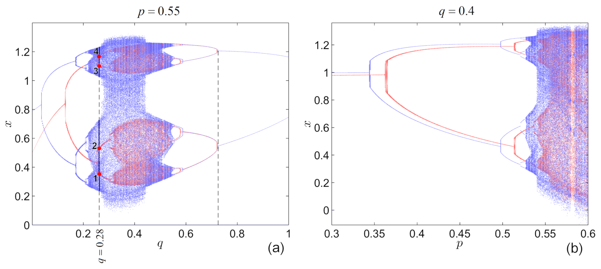
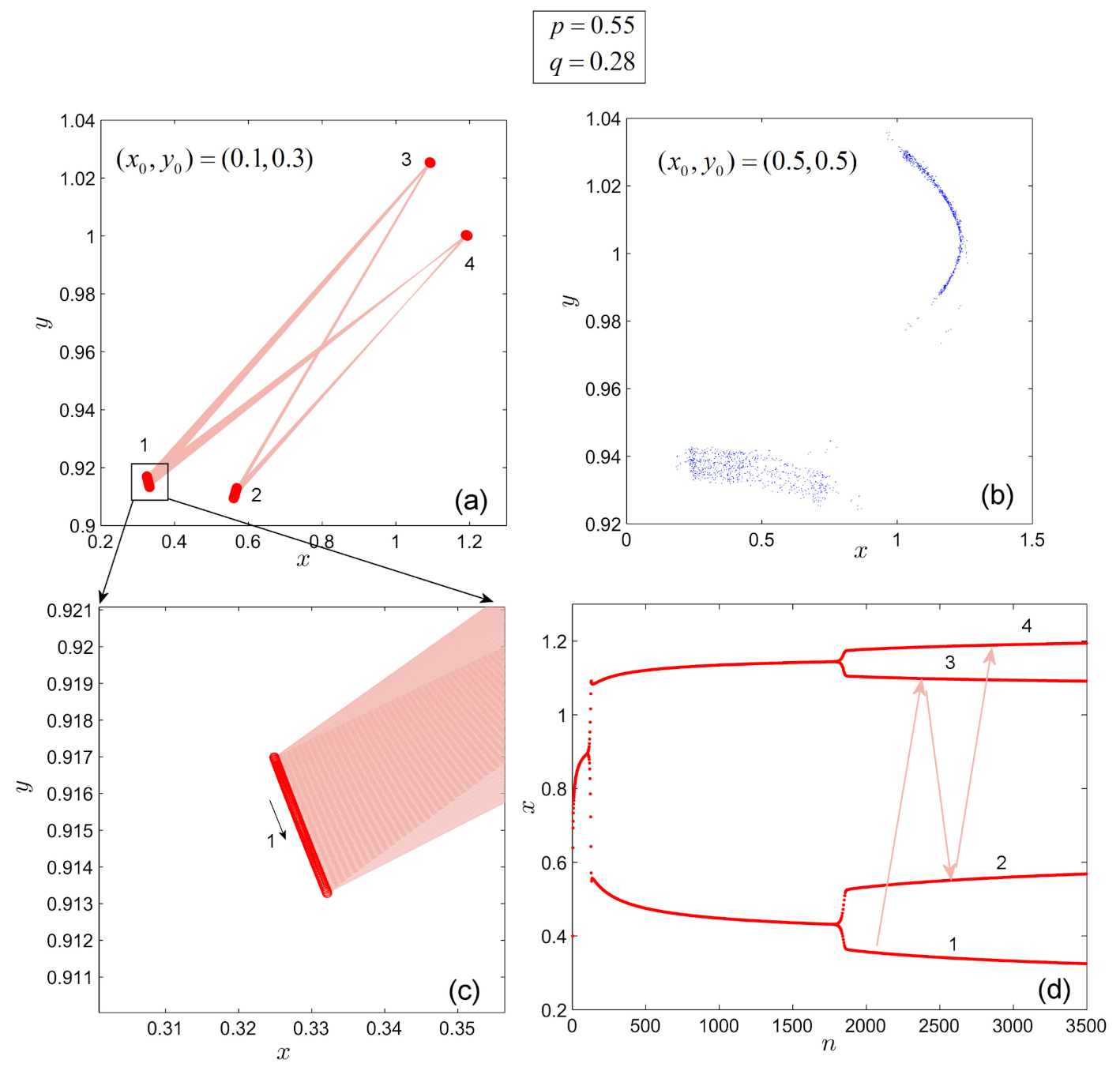
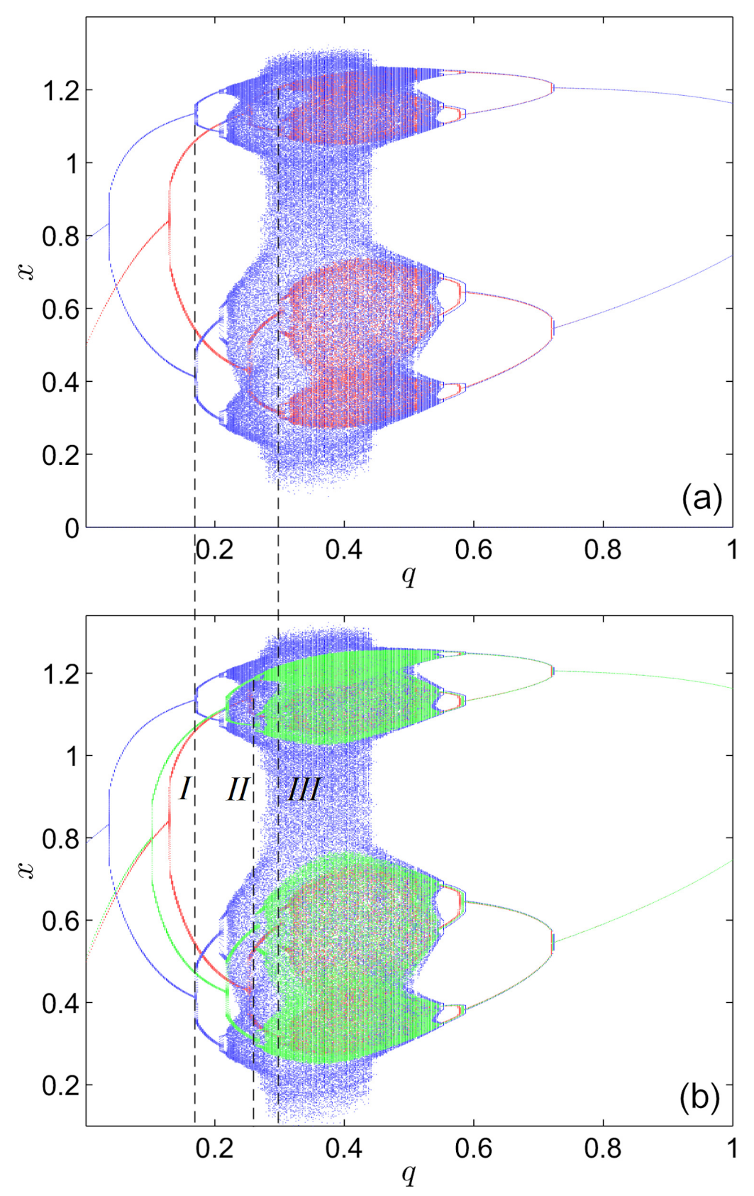
The shapes of BSs approximately preserve the shapes for different initial conditions, but move along the p-axis.

(ii)

This delay-like phenomenon with respect to the initial conditions (the BSs seem to move “forward” or “backward” on the BDs (see the dotted lines I, $II$, and $III$ in Figure 5, as the initial conditions are changing) was already found in a continuous-time FO system [47], where the “delay” was observed with respect to the integration step-size of the numerical method used.

(iii)

It is interesting to compare the above results with the case of the Feigenbaum attractor of the IO logistic map $x(n+1)=px\left(n\right)(1-x(n\left)\right)$, for the limiting value $p_{\infty }=3.569946\dots$ [48], which, however, is not an attracting set and for which there is no sensitive dependence on initial conditions.

By summarizing the investigation in this work, it is concluded that, because of the mentioned dependence on initial conditions, it is impossible to find hidden attractors in the FO system (8) by numerically searching the paths of system orbits by testing initial conditions within neighborhoods of equilibria.

5. Discussion

In this paper, the system of coupled logistic maps modeled by Caputo’s delta fractional difference was studied, both analytically and numerically. The system boundedness and global dynamics were analyzed in detail. Extensive numerical simulations were performed on the system dynamics, revealing the impossibility of finding hidden attractors by numerically testing the orbits starting from initial conditions within neighborhoods of equilibria. The main reason appears to be that, at least for the considered system, the BSs forming the BDs for small values of q (about $q<0.75$) are different for different initial conditions; thereby, the existence of hidden attractors cannot be realized numerically, as typical for continuous integer-order systems. It seems that the coexistence of attractors as necessary for the existence of hidden attractors cannot be well-defined for such a discrete fractional-order system, perhaps also for other discrete fractional-order systems. In general, the phenomenon of “coexistence of attractors” for discrete fractional-order systems needs further investigation.

A possible future research direction is to consider k-periodic problems given by the condition $u\left(k\right)=u\left(0\right)$ for $k\ge 1$, regarding the existence, uniqueness, and bifurcation of solutions, similarly to the periodic boundary value problem $x\left(0\right)=x\left(T\right)$ for functional differential equations [49,50,51].

References

1. Oldham, K.; Spanier, J. The Fractional Calculus: Theory and Applications of Differentiation and Integration to Arbitrary Order; Academic Press: New York, NY, USA, 1974. [Google Scholar]
2. Podlubny, I. Geometric and physical interpretation of fractional integration and fractional differentiation. Fract. Calc. Appl. Anal. 2002, 5, 367–386. [Google Scholar]
3. Li, H.-L.; Jiang, H.; Cao, J. Global synchronization of fractional-order quaternion-valued neural networks with leakage and discrete delays. Neurocomputing 2020, 385, 211–219. [Google Scholar] [CrossRef]
4. Ray, S.A.; Atangana, A.; Noutchie, S.C.O.; Kurulay, M.; Bildik, N.; Kilicman, A. Fractional calculus and its applications in applied mathematics and other sciences. Math. Probl. Eng. 2014, 2014, 849395. [Google Scholar] [CrossRef]
5. Kang, Y.M.; Xie, Y.; Lu, J.; Jiang, J. On the nonexistence of non-constant exact periodic solutions in a class of the Caputo fractional-order dynamical systems. Nonlinear Dyn. 2015, 82, 1259–1267. [Google Scholar] [CrossRef]
6. Tavazoei, M.; Haeri, M. A proof for non existence of periodic solutions in time invariant fractional order systems. Automatica 2009, 45, 1886–1890. [Google Scholar] [CrossRef]
7. Tavazoei, M. A note on fractional-order derivatives of periodic functions. Automatica 2010, 46, 945–948. [Google Scholar] [CrossRef]
8. Yazdani, M.; Salarieh, H. On the existence of periodic solutions in time-invariant fractional order systems. Automatica 2011, 47, 1834–1837. [Google Scholar] [CrossRef]
9. Shen, J.; Lam, J. Non-existence of finite-time stable equilibria in fractional-order nonlinear systems. Automatica 2014, 50, 547–551. [Google Scholar] [CrossRef]
10. Fečkan, M. Note on periodic and asymptotically periodic solutions of fractional differential equations. Stud. Syst. Decis. Control 2020, 177, 153–185. [Google Scholar]
11. Kaslik, E.; Sivasundaram, S. Non-existence of periodic solutions in fractional-order dynamical systems and a remarkable difference between integer and fractional-order derivatives of periodic functions. Nonlinear Anal. Real World Appl. 2012, 13, 1489–1497. [Google Scholar] [CrossRef] [Green Version]
12. Area, I.; Losada, J.; Nieto, J. On Fractional Derivatives and Primitives of Periodic Functions. Abstr. Appl. Anal. 2014, 2014, 392598. [Google Scholar] [CrossRef] [Green Version]
13. Diblík, J.; Fečkan, M.; Pospisil, M. Nonexistence of periodic solutions and S-asymptotically periodic solutions in fractional difference equations. Appl. Math. Comput. 2015, 257, 230–240. [Google Scholar] [CrossRef]
14. Bin, H.; Huang, L.; Zhang, G. Convergence and periodicity of solutions for a class of difference systems. Adv. Differ. Equ. 2006, 2006, 70461. [Google Scholar] [CrossRef] [Green Version]
15. Jonnalagadda, J. Periodic solutions of fractional nabla difference equations. Commun. Appl. Anal. 2016, 20, 585–610. [Google Scholar]
16. Edelman, M. Cycles in asymptotically stable and chaotic fractional maps. Nonlinear Dyn. 2021, 104, 2829–2841. [Google Scholar] [CrossRef]
17. Pospíšil, M. Note on fractional difference equations with periodic and S-asymptotically periodic right-hand side. Nonlinear Oscil. 2021, 24, 99–109. [Google Scholar]
18. Danca, M.F.; Fečkan, M.; Kuznetsov, N.V.; Chen, G. Fractional-order PWC systems without zero Lyapunov exponents. Nonlinear Dyn. 2018, 92, 1061–1078. [Google Scholar] [CrossRef]
19. Leonov, G.; Kuznetsov, N. Hidden attractors in dynamical systems. From hidden oscillations in Hilbert-Kolmogorov, Aizerman, and Kalman problems to hidden chaotic attractors in Chua circuits. Int. J. Bifurc. Chaos Appl. Sci. Eng. 2013, 23, 1330002. [Google Scholar] [CrossRef] [Green Version]
20. Leonov, G.; Kuznetsov, N.; Mokaev, T. Homoclinic orbits, and self-excited and hidden attractors in a Lorenz-like system describing convective fluid motion. Eur. Phys. J. Spec. Top. 2015, 224, 1421–1458. [Google Scholar] [CrossRef] [Green Version]
21. Kuznetsov, N. Theory of hidden oscillations and stability of control systems. J. Comput. Syst. Sci. Int. 2020, 59, 647–668. [Google Scholar] [CrossRef]
22. Danca, M.F.; Kuznetsov, N.; Chen, G. Approximating hidden chaotic attractors via parameter switching. Chaos 2018, 28, 5007925. [Google Scholar] [CrossRef]
23. Danca, M.F. Hidden chaotic attractors in fractional-order systems. Nonlinear Dyn. 2017, 89, 577–586. [Google Scholar] [CrossRef] [Green Version]
24. Danca, M.F.; Bourke, P.; Kuznetsov, N. Graphical structure of attraction basins of hidden attractors: The Rabinovich-Fabrikant system. Int. J. Bifurc. Chaos 2019, 29, 1930001. [Google Scholar] [CrossRef] [Green Version]
25. Danca, M.F.; Kuznetsov, N.; Chen, G. Unusual dynamics and hidden attractors of the Rabinovich–Fabrikant system. Nonlinear Dyn. 2017, 88, 791–805. [Google Scholar] [CrossRef]
26. Danca, M.F. Hidden transient chaotic attractors of Rabinovich–Fabrikant system. Nonlinear Dyn. 2016, 86, 1263–1270. [Google Scholar] [CrossRef] [Green Version]
27. Danca, M.F.; Kuznetsov, N. Hidden chaotic sets in a Hopfield neural system. Chaos Solitons Fractals 2017, 103, 144–150. [Google Scholar] [CrossRef]
28. Danca, M.F. Coexisting Hidden and self-excited attractors in an economic system of integer or fractional order. Int. J. Bifurc. Chaos 2021, 31, 2150062. [Google Scholar] [CrossRef]
29. Danca, M.F.; Fečkan, M.; Kuznetsov, N.; Chen, G. Complex dynamics, hidden attractors and continuous approximation of a fractional-order hyperchaotic PWC system. Nonlinear Dyn. 2018, 91, 2523–2540. [Google Scholar] [CrossRef] [Green Version]
30. Jafari, S.; Sprott, J.; Nazarimehr, F. Recent new examples of hidden attractors. Eur. Phys. J. Spec. Top. 2015, 224, 1469–1476. [Google Scholar] [CrossRef]
31. Diethelm, K.; Ford, N.; Freed, A. A predictor-corrector approach for the numerical solution of fractional differential equations. Nonlinear Dyn. 2002, 29, 3–22. [Google Scholar] [CrossRef]
32. Garrappa, R. Numerical solution of fractional differential equations: A survey and a software tutorial. Mathematics 2018, 6, 16. [Google Scholar] [CrossRef] [Green Version]
33. Kuttner, B. On differences of fractional order. Proc. Lond. Math. Soc. 1957, 3, 453–466. [Google Scholar] [CrossRef]
34. Wang, Q.; Lu, D.; Fang, Y. Stability analysis of impulsive fractional differential systems with delay. Appl. Math. Lett. 2015, 40, 1–6. [Google Scholar] [CrossRef]
35. Wu, G.C.; Baleanu, D. Stability analysis of impulsive fractional difference equations. Fract. Calc. Appl. Anal. 2018, 21, 354–375. [Google Scholar] [CrossRef]
36. Edelman, M. On stability of fixed points and chaos in fractional systems. Chaos 2018, 28, 023112. [Google Scholar] [CrossRef] [PubMed]
37. Lopez-Ruiz, R.; Fournier-Prunaret, D. Indirect Allee effect, bistability and chaotic oscillations in a predator-prey discrete model of logistic type. Chaos Solitons Fractals 2005, 24, 85–101. [Google Scholar] [CrossRef]
38. Abdeljawad, T. On Riemann and Caputo fractional differences. Comput. Math. Appl. 2011, 62, 1602–1611. [Google Scholar] [CrossRef] [Green Version]
39. Atici, F.M.; Eloe, P.W. Discrete fractional calculus with the nabla operator. Electron. J. Qual. Theory Differ. Equ. 2009, 3, 1–12. [Google Scholar] [CrossRef]
40. Anastassiou, G.A. Discrete fractional calculus and inequalities. arXiv 2009, arXiv:0911.3370. [Google Scholar]
41. Chen, F.; Luo, X.; Zhou, Y. Existence Results for Nonlinear Fractional Difference Equation. Adv. Differ. Equ. 2011, 2011, 713201. [Google Scholar] [CrossRef] [Green Version]
42. Danca, M.F.; Fečkan, M.; Kuznetsov, N. Chaos control in the fractional order logistic map via impulses. Nonlinear Dyn. 2019, 98, 1219–1230. [Google Scholar] [CrossRef] [Green Version]
43. Anh, P.; Babiarz, A.; Czornik, A.; Niezabitowski, M.; Siegmund, S. Asymptotic properties of discrete linear fractional equations. Bull. Pol. Acad. Sci. Tech. Sci. 2019, 67, 749–759. [Google Scholar]
44. Čermak, J.; Gyǒri, I.; Nechvátal, L. On explicit stability conditions for a linear fractional difference system. Fract. Calc. Appl. Anal. 2015, 18, 651–672. [Google Scholar] [CrossRef]
45. Danca, M.F. Puu system of fractional order and its chaos suppression. Symmetry 2020, 12, 340. [Google Scholar] [CrossRef] [Green Version]
46. Wu, G.C.; Baleanu, D. Discrete chaos in fractional delayed logistic maps. Nonlinear Dyn. 2015, 80, 1697–1703. [Google Scholar] [CrossRef]
47. Danca, M.F. Hopfield neuronal network of fractional order: A note on its numerical integration. Chaos Solitons Fractals 2021, 151, 111219. [Google Scholar] [CrossRef]
48. Eckmann, J.P.; Ruelle, D. Ergodic theory of chaos and strange attractors. Rev. Mod. Phys. 1985, 57, 617–656. [Google Scholar] [CrossRef]
49. Fečkan, M.; Marynets, K. Approximation approach to periodic BVP for fractional differential systems. Eur. Phys. J. Spec. Top. 2017, 226, 3681–3692. [Google Scholar] [CrossRef]
50. Fečkan, M.; Marynets, K. Approximation approach to periodic BVP for mixed fractional differential systems. J. Comput. Appl. Math. 2018, 339, 208–217. [Google Scholar] [CrossRef]
51. Feckan, M.; Marynets, K.; Wang, J. Periodic boundary value problems for higher-order fractional differential systems. Math. Methods Appl. Sci. 2019, 42, 3616–3632. [Google Scholar] [CrossRef]
Figure 1. Stability regions of equilibria. (a) Stability region of E 1 (grey plot); (b) Stability region of E 5 (grey plot); (c) Instability region of all equilibria (light red plot); (d) Phase plot of a representative orbit from the point within the stability region of E 1 , with p = 0.5 and q = 0.5 (Figure 1a) from initial condition close to E 1 ; (e) phase plot of a representative orbit from a point within the stability region of E 1 , with p = 0.1 and q = 0.5 (Figure 1b) from initial condition close to E 5 .
Mathematics 09 02204 g001
Figure 2. (a) The BD for p = 0.55 vs. q obtained for ( x 0 , y 0 ) = ( 0.1 , 0.3 ) ; (b) the BD and for q = 0.4 vs. p ( 0.3 , 0.6 ) for ( x 0 , y 0 ) = ( 0.1 , 0.3 ) .
Mathematics 09 02204 g002
Figure 3. (a) The BD for p = 0.55 vs. q with two BSs: one obtained for ( x 0 , y 0 ) = ( 0.1 , 0.3 ) , in Figure 2a (red plot), and one for a second initial condition ( x 0 , y 0 ) = ( 0.5 , 0.5 ) (blue plot); (b) the BD for q = 0.4 vs. p ( 0.3 , 0.6 ) with two BSs: one for ( x 0 , y 0 ) = ( 0.1 , 0.3 ) , in Figure 2b (red plot), and a new one for ( x 0 , y 0 ) = ( 0.9 , 0.6 ) (blue plot). Dotted line in the BD in Figure 2b indicates the existence of two different attractors: a four-periodic-like orbit (red bullets) and a two-period chaotic band orbit (dark blue segments).
Mathematics 09 02204 g003
Figure 4. Two attractors for p = 0.55 and q = 0.28 : (a) The four-periodic-like attractor for ( x 0 , y 0 ) = ( 0.1 , 0.3 ) ; (b) the two-period chaotic-like attractor for ( x 0 , y 0 ) = ( 0.5 , 0.5 ) ; (c) zoomed region around the point 1 of the periodic-like orbit underlines the slow convergence of the orbit; (d) time series of the periodic-like orbit.
Mathematics 09 02204 g004
Figure 5. The BDs of system (8) for p = 0.55 . (a) Initial conditions ( 0.1 , 0.3 ) (red BS) and ( 0.5 , 0.5 ) (blue BS); (b) Initial conditions ( 0.1 , 0.3 ) (red BS), ( 0.5 , 0.5 ) (blue BS) and ( 0.01 , 0.7 ) (green plot).
Mathematics 09 02204 g005
Figure 6. The BDs of system (8) for p = 0.55 , obtained with the same three different initial conditions but with different maximum iteration numbers: (a) 3500 iterations; (b) 5000 iterations.
Mathematics 09 02204 g006