Common Positive Solution of Two Nonlinear Matrix Equations Using Fixed Point Results

Abstract

We discuss a pair of nonlinear matrix equations (NMEs) of the form $\mathcal{X}=R_1+{\sum }_{i=1}^k{\mathcal{A}}_i^{*}F\left(\mathcal{X}\right){\mathcal{A}}_i$, $\mathcal{X}=R_2+{\sum }_{i=1}^k{\mathcal{B}}_i^{*}G\left(\mathcal{X}\right){\mathcal{B}}_i$, where $R_1,R_2\in \mathcal{P}\left(n\right)$, ${\mathcal{A}}_i,{\mathcal{B}}_i\in \mathcal{M}\left(n\right)$, $i=1,\cdots ,k$, and the operators $F,G:\mathcal{P}\left(n\right)\to \mathcal{P}\left(n\right)$ are continuous in the trace norm. We go through the necessary criteria for a common positive definite solution of the given NME to exist. We develop the concept of a joint Suzuki-implicit type pair of mappings to meet the requirement and achieve certain existence findings under weaker assumptions. Some concrete instances are provided to show the validity of our findings. An example is provided that contains a randomly generated matrix as well as convergence and error analysis. Furthermore, we offer graphical representations of average CPU time analysis for various initializations.

1. Introduction and Preliminaries

Nonlinear matrix equations have long been a popular topic in nonlinear analysis. Control theory, dynamical programming, stochastic filtering, queuing theory, statistics, and a variety of other mathematical and physical fields use these equations regularly. Using partially ordering and the traditional Banach contraction theorem, Ran and Reurings [1,2] investigated the existence of solutions to matrix problems (in short, BCT). Turinici in [3] is a good place to start for early results in this regard. Indeed, Ran and Reurings [1] and Nieto and Rodriguez-Lopez [4,5] reinvestigated and examined this field (see also [6]). Abbas et al. [7] examined the occurrence of fixed points of T-Ćirić-type mappings in partially ordered spaces. For nonlinear contractions under symmetric closure of an arbitrary relation, Samet and Turinici [8] achieved some findings. Ahmadullah et al. [9,10,11,12] and Alam and Imdad [13] have recently utilized a binary relation to show a relation-theoretic counterpart of the BCT that unifies certain well-known relevant order-theoretic fixed point findings. Suzuki [14], on the other hand, discovered a surprising generalization of the BCT that describes metric completeness, i.e., a metric space is complete if and only if every Suzuki-type mapping has a fixed point in it.

Motivated by the preceding work, we present the concept of joint Suzuki-implicit type pair of mappings on arbitrary binary relation and establish certain existence findings under weaker assumptions. We provide some instance cases to show the veracity of our findings. We then apply these findings to nonlinear matrix equations. We also explore the convergence behavior of various initializations with graphical representations using MATLAB.

For the purpose of thoroughness, we will now review some notation, definitions, and outcomes. Throughout this article, the notations $\mathbb{Z},\mathbb{N},\mathbb{R},{\mathbb{R}}_{+}$ have their usual meanings, and ${\mathbb{N}}^{*}=\mathbb{N}\cup \left\{0\right\}$.

We call $(\Xi ,\mathfrak{R})$ a relational set if (i) $\Xi \ne \varnothing$ is a set and (ii) $\mathfrak{R}$ is a binary relation on $\Xi$.

In addition, if $(\Xi ,d)$ is a metric space, we call $(\Xi ,d,\mathfrak{R})$ a relational metric space (RMS, for short).

The following are some standard terms used in the theory of relational sets (see, e.g., [8,13,15,16,17]).

Let $(\Xi ,\mathfrak{R})$ be a relational set, $(\Xi ,d,\mathfrak{R})$ be an RMS, and let $\mathcal{T},\mathcal{S}$ be self-mappings on $\Xi$. Then:

• $\nu \in \Xi$ is $\mathfrak{R}$-related to $\vartheta \in \Xi$ if and only if $(\nu ,\vartheta )\in \mathfrak{R}$;
• The set $(\Xi ,\mathfrak{R})$ is said to be complete if for all $\nu ,\vartheta \in \Xi ,[\nu ,\vartheta ]\in \mathfrak{R}$, where $[\nu ,\vartheta ]\in \mathfrak{R}$ means that either $(\nu ,\vartheta )\in \mathfrak{R}$ or $(\vartheta ,\nu )\in \mathfrak{R}$;
• A sequence $\left({\nu }_n\right)$ in $\Xi$ is said to be $\mathfrak{R}$-preserving if $({\nu }_n,{\nu }_{n+1})\in \mathfrak{R}$, $\forall n\in {\mathbb{N}}^{*}$;
• $(\Xi ,d,\mathfrak{R})$ is said to be $\mathfrak{R}$-complete if every $\mathfrak{R}$-preserving Cauchy sequence converges in X;
• $\mathfrak{R}$ is said to be $\mathcal{T}$-closed if $(\nu ,\vartheta )\in \mathfrak{R}\Rightarrow (\mathcal{T}\nu ,\mathcal{T}\vartheta )\in \mathfrak{R}$. It is said to be weakly $\mathcal{T}$-closed if $(\nu ,\vartheta )\in \mathfrak{R}\Rightarrow [\mathcal{T}\nu ,\mathcal{T}\vartheta ]\in \mathfrak{R}$;
• $\mathfrak{R}$ is said to be d-self-closed if for every $\mathfrak{R}$-preserving sequence with ${\nu }_n\to \nu$, there is a subsequence $\left({\nu }_{n_k}\right)$ of $\left({\nu }_n\right)$, such that $[{\nu }_{n_k},\nu ]\in \mathfrak{R}$, for all $k\in {\mathbb{N}}^{*}$;
• A subset $\mathfrak{Z}$ of $\Xi$ is called $\mathfrak{R}$-directed if for each $\nu ,\vartheta \in \mathfrak{Z}$, there exists $\mu \in \Xi$ such that $(\nu ,\mu )\in \mathfrak{R}$ and $(\vartheta ,\mu )\in \mathfrak{R}$. It is called $(\mathcal{T},\mathfrak{R})$-directed if for each $\nu ,\vartheta \in \mathfrak{Z}$, there exists $\mu \in \Xi$ such that $(\nu ,\mathcal{T}\mu )\in \mathfrak{R}$ and $(\vartheta ,\mathcal{T}\mu )\in \mathfrak{R}$;
• $\mathcal{T}$ is said to be $\mathfrak{R}$-continuous at $\nu$ if for every $\mathfrak{R}$-preserving sequence $\left({\nu }_n\right)$ converging to $\nu$, we get $\mathcal{T}\left({\nu }_n\right)\to \mathcal{T}\left(\nu \right)$ as $n\to \infty$. Moreover, $\mathcal{T}$ is said to be $\mathfrak{R}$-continuous if it is $\mathfrak{R}$-continuous at every point of $\Xi$;
• For $\nu ,\vartheta \in \Xi$, a path of length k (where k is a natural number) in $\mathfrak{R}$ from $\nu$ to $\vartheta$ is a finite sequence $\{{\mu }_0,{\mu }_1,{\mu }_2,\dots ,{\mu }_k\}\subset \Xi$ satisfying the following conditions:

  (i)

  $z_0=\nu$ and ${\mu }_k=\vartheta$,

  (ii)

  $({\mu }_i,{\mu }_{i+1})\in \mathfrak{R}$ for each i$(0\le i\le k-1)$,

  then this finite sequence is called a path of length k joining $\nu$ to $\vartheta$ in $\mathfrak{R}$;
• If for a pair of $\nu ,\vartheta \in \Xi$, there is a finite sequence $\{{\mu }_0,{\mu }_1,{\mu }_2,\dots ,{\mu }_k\}\subset \Xi$ satisfying the following conditions:

  (i)

  $\mathcal{T}{\mu }_0=\nu$ and $\mathcal{T}{\mu }_k=\vartheta$,

  (ii)

  $(\mathcal{T}{\mu }_i,\mathcal{T}{\mu }_{i+1})\in \mathfrak{R}$ for each i $(0\le i\le k-1)$,

  then this finite sequence is called a $\mathcal{T}$-path of length k joining $\nu$ to $\vartheta$ in $\mathfrak{R}$.
  Notice that a path of length k involves $k+1$ elements of $\Xi$, although they are not necessarily distinct;
• $\mathfrak{R}$ on $\Xi$ is called $(\mathcal{T},\mathcal{S})$-closed if $(\mathcal{T}\nu ,\mathcal{T}\vartheta )\in \mathfrak{R}$ whenever $(\mathcal{S}\nu ,\mathcal{S}\vartheta )\in \mathfrak{R}$, for all $\nu ,\vartheta \in \mathcal{X}$.
• A subset $\mathfrak{Z}$ of $\Xi$ is called $(\mathcal{S},\mathfrak{R})$-directed if for each $\nu ,\vartheta \in \mathfrak{Z}$, there exists $\mu \in \Xi$ such that $(\nu ,\mathcal{S}\mu )\in \mathfrak{R}$ and $(\vartheta ,\mathcal{S}\mu )\in \mathfrak{R}$;
• $\mathcal{T}$ is said to be $(\mathcal{S},\mathfrak{R})$-continuous at $\nu$ if for every $\mathfrak{R}$-preserving sequence $\left(\mathcal{S}{\nu }_n\right)$ converging to $\mathcal{S}\nu$, we get $\mathcal{T}\left({\nu }_n\right)\to \mathcal{T}\left(\nu \right)$ as $n\to \infty$. Moreover, $\mathcal{T}$ is said to be $(\mathcal{S},\mathfrak{R})$-continuous if it is $(\mathcal{S},\mathfrak{R})$-continuous at every point of $\Xi$;
• $\mathcal{T}$ and $\mathcal{S}$ are said to be $\mathfrak{R}$-compatible if ${lim}_{n\to \infty }d(\mathcal{S}\left(\mathcal{T}{\nu }_n\right),\mathcal{T}\left(\mathcal{S}{\nu }_n\right))=0$, whenever ${lim}_{n\to \infty }\mathcal{S}\left({\nu }_n\right)={lim}_{n\to \infty }\mathcal{T}\left({\nu }_n\right)$, for any sequence $\left\{{\nu }_n\right\}\subset \Xi$ such that the sequences $\left\{\mathcal{T}{\nu }_n\right\}$ and $\left\{\mathcal{S}{\nu }_n\right\}$ are $\mathfrak{R}$-preserving;
• For a pair of $\nu ,\vartheta \in \Xi$, there is a finite sequence $\{{\omega }_0,{\omega }_1,{\omega }_2,\dots ,{\omega }_k\}\subset \Xi$ satisfying the following conditions:

  (i)

  $\mathcal{S}{\omega }_0=\nu$ and $\mathcal{S}{\omega }_k=\vartheta$,

  (ii)

  $(\mathcal{S}{\omega }_i,\mathcal{S}{\omega }_{i+1})\in \mathfrak{R}$ for each i$(0\le i\le k-1)$,

  then this finite sequence is called a $\mathcal{S}$-path of length k joining $\nu$ to $\vartheta$ in $\mathfrak{R}$.

Proposition 1

([13]). Let $\mathfrak{R}$ be a binary relation defined on a non-empty set Ξ. Then, $(\nu ,\vartheta )\in {\mathfrak{R}}^s\iff [\nu ,\vartheta ]\in \mathfrak{R}$.

We fix following notations for $(\Xi ,\mathfrak{R})$ a relational space, self-mappings $\mathcal{T},\mathcal{S}$ on $\Xi$ and a $\mathfrak{R}$-directed subset $\mathfrak{D}$ of $\Xi$,

(i)

$Fix\left(\mathcal{T}\right):=$ the set of all fixed points of $\mathcal{T}$;

(ii)

$\mathfrak{X}(\mathcal{T},\mathfrak{R}):=\{\nu \in \Xi :(\nu ,\mathcal{T}\nu )\in \mathfrak{R}\}$;

(iii)

$\mathfrak{P}(\nu ,\vartheta ,\mathfrak{R}):=$ the class of all paths in $\mathfrak{R}$ from $\nu$ to $\vartheta$ in $\mathfrak{R}$, where $\nu ,\vartheta \in \Xi$;

(iv)

${\mathfrak{P}}_S(\nu ,\vartheta ,\mathfrak{R}):=$ the class of all $\mathcal{S}$-paths in $\mathfrak{R}$ from $\nu$ to $\vartheta$ in $\mathfrak{R}$, where $\nu ,\vartheta \in \Xi$;

(v)

${\mathfrak{P}}_S(\nu ,\vartheta ,\mathcal{T},\mathfrak{R}):=$ the class of all $\mathcal{S}$-paths $\{{\omega }_0,{\omega }_1,{\omega }_2,\dots ,{\omega }_{\ell }\}$ joining $\nu$ to $\vartheta$ in $\mathfrak{R}$ such that $[\mathcal{S}{\omega }_i,\mathcal{T}{\omega }_i]\in \mathfrak{R}$ for each $i\in \{1,2,3,\dots ,\ell -1\}$;

(vi)

$CFix(\mathcal{T},\mathcal{S}):=$ the set of all common fixed points of $\mathcal{T}$ and $\mathcal{S}$;

(vii)

$COP(\mathcal{T},\mathcal{S}):=$ the set of all coincidence points of $\mathcal{T}$ and $\mathcal{S}$;

(viii)

$\mathfrak{X}(\mathcal{T},\mathcal{S},\mathfrak{R}):=\{\nu \in \Xi :(\mathcal{S}\nu ,\mathcal{T}\nu )\in \mathfrak{R}\}$;

(ix)

$\Delta (\mathfrak{D},\mathcal{S},\mathfrak{R}):={\bigcup }_{\nu ,\vartheta \in \mathfrak{D}}\{\mu \in \Xi :(\nu ,\mathcal{S}\mu )\in \mathfrak{R}\mathrm{and}(\vartheta ,\mathcal{S}\mu )\in \mathfrak{R}\}$.

To complete the main result, we need:

Lemma 1

([18]). Let g be a self-mapping defined on a set $\Xi \ne \varnothing$. Then, there exists a subset $\mathfrak{Z}\subseteq \Xi$ with $g\left(\mathfrak{Z}\right)=g(\Xi )$ and $g:\mathfrak{Z}\to \Xi$ is one-one.

2. Joint Suzuki-Implicit Type Results on Relational Metric Spaces

Let $\Phi$ be the class of functions $\phi :{\mathbb{R}}_{+}\to {\mathbb{R}}_{+}$ satisfying the following conditions:

(i)

$\phi$ is increasing and $\phi \left(0\right)=0$;

(ii)

${\sum }_{n=1}^{\infty }{\phi }^n\left(\zeta \right)<\infty$, for $\zeta >0$; where ${\phi }^n$ is $n^{\mathrm{th}}$-iterate.

It should be noted that $\phi \left(\zeta \right)<\zeta$ and the family $\Phi \ne \varnothing$.

Example 1.

Consider $(\Xi ,d)$ with usual metric, where $\Xi =[0,1]$. Define the mapping $\phi \left(\zeta \right)=\frac{2\lambda \zeta }{9}$, where $0<\lambda <1$. Then, we have ${\phi }^n\left(\zeta \right)\le \frac{2^n{\lambda }^n\zeta }{9^n}$. Therefore, ${\sum }_{n=1}^{\infty }{\phi }^n\left(\zeta \right)={\sum }_{n=1}^{\infty }\frac{2^n{\lambda }^n\zeta }{9^n}<\infty$ and hence $\Phi \ne \varnothing$.

Let $\mathfrak{G}:=\{\mathcal{G}:{\mathbb{R}}_{+}^6\to \mathbb{R}\mathrm{is}\mathrm{lower}\mathrm{semi}-\mathrm{continuous}(\mathrm{l}.\mathrm{s}.\mathrm{c}.)\mathrm{real}\mathrm{valued}\mathrm{function}\}$ satisfy the following conditions:

(${\mathcal{G}}_1$)

$\mathcal{G}(\zeta ,\xi ,\xi ,\zeta ,\mu ,0)\le 0$ for all $\zeta ,\xi ,\mu \ge 0$, implies that there exists $\phi \in \Phi$ such that $\zeta \le \phi \left(\xi \right)$;

(${\mathcal{G}}_2$)

$\mathcal{G}(\zeta ,0,0,\zeta ,\zeta ,0)>0$, for all $\zeta >0$.

Let ${\mathfrak{G}}^{\prime }:=\{\mathcal{G}\in \mathfrak{G}\}$ and following additional conditions hold:

(${\mathcal{G}}_3$)

$\mathcal{G}(\zeta ,\zeta ,0,0,\zeta ,\zeta )>0$, for all $\zeta >0$.

Obviously, $\mathfrak{G}$ is more general than ${\mathfrak{G}}^{\prime }$.

The following examples are inspired from [19,20].

Example 2.

Let $\mathcal{G}(r_1,r_2,r_3,r_4,r_5,r_6)=r_1-amax\{r_2,r_3,r_4\}+b(r_5+r_6)$, $0\le a<1$ and $b>0$.

(${\mathcal{G}}_1$)

For $\zeta ,\xi ,\mu \ge 0$, we have

$$\mathcal{G}(\zeta ,\xi ,\xi ,\zeta ,\mu ,0)=\zeta -amax\{\xi ,\xi ,\zeta \}+b\mu \le 0.$$

If $\xi \le \zeta$, then $(1-a)\zeta <0$, a contradiction as $a\in [0,1)$. Therefore, $\zeta \le \phi \left(\xi \right)$, where $\phi \left(\xi \right)=h\xi$ ($0<h<1$).

(${\mathcal{G}}_2$)

$\mathcal{G}(\zeta ,0,0,\zeta ,\zeta ,0)=(1-a+b)\zeta >0$ for all $\zeta >0$.

Example 3.

Let $\mathcal{G}(r_1,r_2,r_3,r_4,r_5,r_6)=r_1^2-a{r}_2^2-b\frac{r_3^2+r_4^2}{r_5+r_6+1},0<a,b<1$ and $a+2b<1$.

(${\mathcal{G}}_1$)

For $\zeta ,\xi ,\mu \ge 0$, we have

$$\mathcal{G}(\zeta ,\xi ,\xi ,\zeta ,\mu ,0)={\zeta }^2-a{\xi }^2-b\frac{{\zeta }^2+{\xi }^2}{1+\mu }\le 0,$$

which implies that ${\zeta }^2\le a{\xi }^2+b({\zeta }^2+{\xi }^2)$. Then, ${\zeta }^2\le \left(\frac{a+b}{1-b}\right){\xi }^2$. Hence, $\zeta \le \phi \left(\xi \right)$, where $\phi \left(\xi \right)=h\xi$, $h=\sqrt{\frac{a+b}{1-b}}<1$.

(${\mathcal{G}}_2$)

$\mathcal{G}(\zeta ,0,0,\zeta ,\zeta ,0)=\frac{(1-b){\zeta }^2+{\zeta }^3}{1+\zeta }>0$.

Example 4.

Let $\mathcal{G}(r_1,r_2,r_3,r_4,r_5,r_6)=r_1^2-a{r}_2^2-b\frac{r_3^2+r_4^2}{r_5^2+r_6^2+1},0<a,b<1$ and $a+2b<1$,similar to Example 3.

Example 5.

Let $\mathcal{G}(r_1,r_2,r_3,r_4,r_5,r_6)=r_1-a{r}_2-b{r}_3-c\frac{r_4{r}_5}{r_5+r_6+1},0<a,b,c<1$ and $a+b+c<1$.

(${\mathcal{G}}_1$)

For $\zeta ,\xi ,\mu \ge 0$, we have

$$\mathcal{G}(\zeta ,\xi ,\xi ,\zeta ,\mu ,0)=\zeta -a\xi -b\xi -c\frac{\zeta \mu }{1+\mu }\le 0$$

which implies that $\zeta -(a+b)\xi \le c\zeta$, that is, $\zeta \le \phi \left(\xi \right)$, where $\phi \left(\xi \right)=h\xi$, $h=\frac{a+b}{1-c}<1$.

(${\mathcal{G}}_2$)

$\mathcal{G}(\zeta ,0,0,\zeta ,\zeta ,0)=\frac{\zeta +(1-c){\zeta }^2}{1+\zeta }>0$ for all $\zeta >0$.

Example 6.

Let $\mathcal{G}(r_1,r_2,r_3,r_4,r_5,r_6)=r_1-a{r}_2-b\frac{r_3{r}_6}{r_5+r_6+1}-c{r}_4$, $0<a,b,c<1$ and $a+b+c<1$.

(${\mathcal{G}}_1$)

For $\zeta ,\xi ,\mu \ge 0$, we have

$$\mathcal{G}(\zeta ,\xi ,\xi ,\zeta ,\mu ,0)=\zeta -a\xi -c\zeta \le 0$$

which implies that $\zeta -a\xi \le c\zeta$, that is, $\zeta \le \phi \left(\xi \right)$, where $\phi \left(\xi \right)=h\xi$, $h=\frac{a}{1-c}<1$.

(${\mathcal{G}}_2$)

$\mathcal{G}(\zeta ,0,0,\zeta ,\zeta ,0)=(1-c)\zeta >0$ for all $\zeta >0$.

Definition 1.

Let $(\Xi ,d,\mathfrak{R})$ be an RMS and $\mathcal{T},\mathcal{S}:\Xi \to \Xi$ be given mappings. A pair of mappings $(\mathcal{T},\mathcal{S})$ is said to be a joint Suzuki-implicit type mapping if there exists $\mathcal{G}\in \mathfrak{G}$ such that for $(\mathcal{S}\nu ,\mathcal{S}\vartheta )\in \mathfrak{R}$

$$\begin{array}{ccc}\hfill & & \frac{1}{2}d(\mathcal{S}\nu ,\mathcal{T}\nu )\le d(\mathcal{S}\nu ,\mathcal{S}\vartheta )\hfill \\ & & \Rightarrow \mathcal{G}\left(d\right(\mathcal{T}\nu ,\mathcal{T}\vartheta ),d(\mathcal{S}\nu ,\mathcal{S}\vartheta ),d(\mathcal{S}\nu ,\mathcal{T}\nu ),d(\mathcal{S}\vartheta ,\mathcal{T}\vartheta ),d(\mathcal{S}\nu ,\mathcal{T}\vartheta ),d(\mathcal{S}\vartheta ,\mathcal{T}\nu \left)\right)\le 0.\hfill \end{array}$$

(1)

We denote by Υ the collection of all joint Suzuki-implicit type mappings on $(\Xi ,d,\mathfrak{R})$.

Theorem 1.

Let $(\Xi ,d,\mathfrak{R})$ be an RMS and $\mathcal{Y}$ an $\mathfrak{R}$-complete subspace of Ξ. Let $\mathcal{T},\mathcal{S}:\Xi \to \Xi$. Suppose that the following conditions hold:

($C_1$)

$\mathfrak{X}(\mathcal{T},\mathcal{S},\mathfrak{R})\ne \varnothing$;

($C_2$)

$\mathcal{T}(\Xi )\subseteq \mathcal{Y}\cap \mathcal{S}(\Xi )$;

($C_3$)

$\mathfrak{R}$ is $(\mathcal{T},\mathcal{S})$-closed;

($C_4$)

$(\mathcal{T},\mathcal{S})\in {\rm Y}$;

($C_5$)

(a)

$\mathcal{Y}\subseteq \mathcal{S}(\Xi )$,

(b)

$\mathcal{T}$ is $(\mathcal{S},\mathfrak{R})$-continuous or $\mathcal{T}$ and $\mathcal{S}$ are continuous or ${\mathfrak{R}|}_{\mathcal{Y}}$ is d-self-closed.

or, alternatively,

($C_5^{\text{'}}$)

(c)

$\mathcal{T}$ and $\mathcal{S}$ are $\mathfrak{R}$-compatible,

(d)

$\mathcal{T}$ is $\mathfrak{R}$-continuous and either $\mathcal{S}$ is $\mathfrak{R}$-continuous or $(\Xi ,d,\mathfrak{R})$ is $(\mathcal{S},\mathfrak{R})$-regular;

(e)

$\mathcal{S}$ is continuous and either $\mathcal{T}$ is $\mathfrak{R}$-continuous or $\mathfrak{R}$ is $(\mathcal{S},d)$-self-closed.

Then, $COP(\mathcal{T},\mathcal{S})\ne \varnothing$.

Proof. 

By $\left(C_2\right)$, we can define a mapping g on $\Xi$ satisfying $\mathcal{S}g\nu =\mathcal{T}\nu$ for all $\nu \in \Xi$. By $\left(C_1\right)$, $(\mathcal{S}\nu ,\mathcal{S}g\nu )\in \mathfrak{R}$, therefore, from $\left(C_4\right)$, $\frac{1}{2}d(\mathcal{S}\nu ,\mathcal{T}\nu )=\frac{1}{2}d(\mathcal{S}\nu ,\mathcal{S}g\nu )\le d(\mathcal{S}\nu ,\mathcal{S}g\nu )$ holds, which implies that

$$\begin{array}{c}\hfill \begin{array}{c}\mathcal{G}\left(d\right(\mathcal{T}\nu ,\mathcal{T}g\nu ),d(\mathcal{S}\nu ,\mathcal{S}g\nu ),d(\mathcal{S}\nu ,\mathcal{T}\nu ),d(\mathcal{S}g\nu ,\mathcal{T}g\nu ),d(\mathcal{S}\nu ,\mathcal{T}g\nu ),d(\mathcal{S}g\nu ,\mathcal{T}\nu \left)\right)\le 0\\ \Rightarrow \mathcal{G}\left(d\right(\mathcal{S}g\nu ,\mathcal{S}gg\nu ),d(\mathcal{S}\nu ,\mathcal{S}g\nu ),d(\mathcal{S}\nu ,\mathcal{S}g\nu ),d(\mathcal{S}g\nu ,\mathcal{S}gg\nu ),\\ d(\mathcal{S}\nu ,\mathcal{S}gg\nu ),d(\mathcal{S}g\nu ,\mathcal{S}g\nu ))\le 0\\ \Rightarrow \mathcal{G}\left(d\right(\mathcal{S}g\nu ,\mathcal{S}gg\nu ),d(\mathcal{S}\nu ,\mathcal{S}g\nu ),d(\mathcal{S}\nu ,\mathcal{S}g\nu ),d(\mathcal{S}g\nu ,\mathcal{S}gg\nu ),d(\mathcal{S}\nu ,\mathcal{S}gg\nu ),0))\le 0.\end{array}\end{array}$$

It follows from $\left({\mathcal{G}}_1\right)$ that $\phi \in \Phi$, such that

$$d(\mathcal{S}g\nu ,\mathcal{S}gg\nu )\le \phi \left(d\right(\mathcal{S}\nu ,\mathcal{S}g\nu \left)\right)$$

(2)

holds for all $\nu \in \Xi$. Let $\varrho \in \Xi$. Put ${\varrho }_0=\varrho$ and ${\varrho }_n=g^n\varrho$ for all $n\in \mathbb{N}$. Then, ${\varrho }_{n+1}=g{\varrho }_n$ and $\left(C_1\right)$ implies that

$$\mathcal{S}{\varrho }_{n+1}=\mathcal{T}{\varrho }_n\mathrm{for}\mathrm{all}n\in \mathbb{N}.$$

(3)

Using ($C_3$), we have that $(\mathcal{T}{\varrho }_0,{\mathcal{T}}^2{\varrho }_0)\in \mathfrak{R}$. Continuing this process inductively, we obtain

$$({\mathcal{T}}^n{\varrho }_0,{\mathcal{T}}^{n+1}{\varrho }_0)\in \mathfrak{R}$$

for any $n\in {\mathbb{N}}^{*}$. In addition,

$$(\mathcal{S}{\varrho }_n,\mathcal{S}{\varrho }_{n+1})\in \mathfrak{R}$$

(4)

for any $n\in {\mathbb{N}}^{*}$ so that $\left\{\mathcal{S}{\nu }_n\right\}$ is an $\mathfrak{R}$-preserving sequence. By (2), we have

$$\begin{array}{ccc}\hfill d(\mathcal{S}{\varrho }_n,\mathcal{S}{\varrho }_{n+1})& =& d(\mathcal{S}g{\varrho }_{n-1},\mathcal{S}gg{\varrho }_{n-1})\hfill \\ \hfill & \le & \phi \left(d(\mathcal{S}{\varrho }_{n-1},\mathcal{S}g{\varrho }_{n-1})\right)\hfill \\ & =& \phi \left(d(\mathcal{S}{\varrho }_{n-1},\mathcal{S}{\varrho }_n)\right)\hfill \\ \hfill & \le & {\phi }^2\left(d(\mathcal{S}{\varrho }_{n-2},\mathcal{S}{\varrho }_{n-1})\right)\hfill \\ \hfill & ⋮& \\ & =& {\phi }^n\left(d(\mathcal{S}{\varrho }_0,\mathcal{S}{\varrho }_1)\right).\hfill \end{array}$$

(5)

Using Equation (5) and the triangular inequality, for all $n,m\in {\mathbb{N}}^{*}$ with $m>n$,

$$\begin{array}{cc}\hfill d(\mathcal{S}{\varrho }_n,\mathcal{S}{\varrho }_m)& \le d(\mathcal{S}{\varrho }_n,\mathcal{S}{\varrho }_{n+1})+d(\mathcal{S}{\varrho }_{n+1},\mathcal{S}{\varrho }_{n+2})+\cdots +d(\mathcal{S}{\varrho }_{m-1},\mathcal{S}{\varrho }_m)\hfill \\ \hfill & \le \sum _{k=n}^m{\phi }^k(d(\mathcal{S}{\varrho }_0,\mathcal{S}{\varrho }_1)\hfill \\ \hfill & \le \sum _{k\ge n}{\phi }^k(d(\mathcal{S}{\varrho }_0,\mathcal{S}{\varrho }_1)\hfill \\ \hfill & \to 0\mathrm{as}n\to \infty .\hfill \end{array}$$

Therefore, $\left\{\mathcal{S}{\varrho }_n\right\}$ is an $\mathfrak{R}$-preserving Cauchy sequence in $\Xi$. As $\left\{\mathcal{S}{\varrho }_n\right\}\subseteq \mathcal{S}(\Xi )$ and $\left\{\mathcal{S}{\varrho }_n\right\}\subseteq \mathcal{Y}\subseteq \mathcal{S}(\Xi )$ (due to $C_5\left(a\right)$), therefore $\left\{\mathcal{S}{\varrho }_n\right\}$ is an $\mathfrak{R}$-preserving Cauchy sequence in $\mathcal{Y}$. Owing to the $\mathfrak{R}$-completeness of $\Xi$, the existence of $\omega \in \Xi$ with ${lim}_{n\to \infty }\mathcal{S}{\varrho }_n=\omega$ is ensured. Assume $\left(C_5\right)\left(a\right)$. As $\mathcal{Y}\subseteq \mathcal{S}(\Xi )$, there exists some $\rho \in \Xi$ such that

$$\underset{n\to \infty }{lim}\mathcal{S}{\varrho }_n=\rho =\mathcal{S}\omega .$$

(6)

Assume $\left(C_5\right)\left(b\right)$. First, we assume that $\mathcal{T}$ is $(\mathcal{S},\mathfrak{R})$-continuous. By using Equations (4) and (6), we obtain

$$\underset{n\to \infty }{lim}\mathcal{S}{\varrho }_{n+1}=\underset{n\to \infty }{lim}\mathcal{T}{\varrho }_n=\mathcal{T}\omega .$$

By the uniqueness of the limit, we have $\mathcal{T}\omega =\mathcal{S}\omega$, so that $\omega \in COP(\mathcal{S},\mathcal{T})$.

Assume $\left(C_5\right)\left(b\right)$. Suppose that $\mathcal{T}$ and $\mathcal{S}$ are continuous. From Lemma 1, there exists a subset $\mathfrak{Z}\subseteq \Xi$ such that $\mathcal{S}\left(\mathfrak{Z}\right)=\mathcal{S}(\Xi )$ and $\mathcal{S}:\mathfrak{Z}\to \Xi$ is one-one. Now, define $h:\mathcal{S}\left(\mathfrak{Z}\right)\to \mathcal{S}(\Xi )$ by

$$h\left(\mathcal{S}\eta \right)=\mathcal{T}\eta ,\mathrm{for}\mathrm{all}\mathcal{S}\eta \in \mathcal{S}\left(\mathfrak{Z}\right)\mathrm{where}\eta \in \mathfrak{Z}.$$

(7)

Since $\mathcal{S}$ is one-one and $\mathcal{T}(\Xi )\subseteq \mathcal{S}\left(\mathfrak{Z}\right)$, h is well defined. As $\mathcal{T}$ and $\mathcal{S}$ are continuous, so is h. On using the fact $S\left(\mathfrak{Z}\right)=\mathcal{S}(\Xi )$ and the conditions $\left(C_2\right)$ and $\left(C_5\right)\left(a\right)$, we have $\mathcal{T}(\Xi )\subseteq \mathcal{S}\left(\mathfrak{Z}\right)\cap \mathcal{Y}$ and $\mathcal{Y}\subseteq S(\Xi )$ which ensures the availability of a sequence $\left\{{\nu }_n\right\}\subset \mathfrak{Z}$ satisfying Equation (3). Take $\varrho \in \mathfrak{Z}$. Using Equations (6) and (7) and the continuity of h, we obtain

$$\mathcal{T}\varrho =h\left(\mathcal{S}\varrho \right)=h\left(\underset{n\to \infty }{lim}\mathcal{S}{\nu }_n\right)=\underset{n\to \infty }{lim}h\left(\mathcal{S}{\nu }_n\right)=\underset{n\to \infty }{lim}\mathcal{T}{\nu }_n=\mathcal{S}\varrho ,$$

so that $\varrho \in COP(\mathcal{S},\mathcal{T})$.

Next, assume that ${\mathfrak{R}|}_{\mathcal{Y}}$ is d-self-closed. Since $\left\{\mathcal{S}{\varrho }_n\right\}$ is $\mathfrak{R}$-preserving in $\mathcal{Y}$ and $\mathcal{S}{\varrho }_n\to S\varrho$, there is a subsequence $\left\{\mathcal{S}{\varrho }_{n_k}\right\}$ of $\left\{\mathcal{S}{\varrho }_n\right\}$ with $[\mathcal{S}{\varrho }_{n_k},\mathcal{S}\varrho ]{\in \mathfrak{R}|}_{\mathcal{Y}}\subseteq \mathfrak{R}$, for all $k\in {\mathbb{N}}^{*}$. Notice that, for all $k\in {\mathbb{N}}^{*}$, $[\mathcal{S}{\varrho }_{n_k},\mathcal{S}\varrho ]\in \mathfrak{R}$ implies that either $(\mathcal{S}{\varrho }_{n_k},\mathcal{S}\varrho )\in \mathfrak{R}$ or $(\mathcal{S}\varrho ,\mathcal{S}{\varrho }_{n_k})\in \mathfrak{R}$.

Now, we assert that for all $k\in {\mathbb{N}}^{*}$

$$\begin{array}{c}\hfill \frac{1}{2}d(\mathcal{S}{\varrho }_{n_k-1},\mathcal{S}{\varrho }_{n_k})\le d(\mathcal{S}{\varrho }_{n_k-1},\mathcal{S}\varrho )\mathrm{or}\frac{1}{2}d(\mathcal{S}{\varrho }_{n_k},\mathcal{S}{\varrho }_{n_k+1})\le d(\mathcal{S}{\varrho }_{n_k},\mathcal{S}\varrho ).\end{array}$$

(8)

On the contrary, let there exist $\ell \in \mathbb{N}$ such that

$$\begin{array}{c}\hfill \frac{1}{2}d(\mathcal{S}{\varrho }_{n_{\ell }-1},\mathcal{S}{\varrho }_{n_{\ell }})>d(\mathcal{S}{\varrho }_{n_{\ell }-1},\mathcal{S}\varrho )\mathrm{and}\frac{1}{2}d(\mathcal{S}{\varrho }_{n_{\ell }},\mathcal{S}{\varrho }_{n_{\ell }+1})>d(\mathcal{S}{\varrho }_{n_{\ell }},\mathcal{S}\varrho ).\end{array}$$

(9)

Now, from Equations (5) and (9), we have

$$\begin{array}{ccc}\hfill d(\mathcal{S}{\varrho }_{n_{\ell }-1},\mathcal{S}{\varrho }_{n_{\ell }})& \le & d(\mathcal{S}{\varrho }_{n_{\ell }-1},\mathcal{S}\varrho )+d(\mathcal{S}{\varrho }_{n_{\ell }},\mathcal{S}\varrho )\hfill \\ & <& \frac{1}{2}[d(\mathcal{S}{\varrho }_{n_{\ell }-1},\mathcal{S}{\varrho }_{n_{\ell }})+d(\mathcal{S}{\varrho }_{n_{\ell }},\mathcal{S}{\varrho }_{n_{\ell }+1})]\hfill \\ & <& \frac{1}{2}[d(\mathcal{S}{\varrho }_{n_{\ell }-1},\mathcal{S}{\varrho }_{n_{\ell }})+d(\mathcal{S}{\varrho }_{n_{\ell }-1},\mathcal{S}{\varrho }_{n_{\ell }})]\hfill \\ & =& d(\mathcal{S}{\varrho }_{n_{\ell }-1},\mathcal{S}{\varrho }_{n_{\ell }}),\hfill \end{array}$$

a contradiction and, therefore, Equation (8) remains true. This implies that either

$$\frac{1}{2}d(\mathcal{S}{\varrho }_{2n-1},{\mathcal{S}}_{{\varrho }_{2n})}\le d(\mathcal{S}{\varrho }_{2n-1},\mathcal{S}\varrho )\mathrm{or}\frac{1}{2}d(\mathcal{S}{\varrho }_{2n},\mathcal{S}{\varrho }_{2n+1})\le d(\mathcal{S}{\varrho }_{2n},\mathcal{S}\varrho )$$

holds for $n\in \mathbb{N}$. Thus, there exists a subsequence $\left\{n_k\right\}$ of $\left\{n\right\}$ such that $\frac{1}{2}d(\mathcal{S}{\varrho }_{n_k},\mathcal{S}{\varrho }_{n_k+1})\le d(\mathcal{S}{\varrho }_{n_k},\mathcal{S}\varrho )$ for $k\in \mathbb{N}$. Then, $\frac{1}{2}d(\mathcal{S}{\varrho }_{n_k},\mathcal{T}{\varrho }_{n_k})\le d(\mathcal{S}{\varrho }_{n_k},\mathcal{S}\varrho )$ for $k\in \mathbb{N}$.

Applying the condition $\left(C_4\right)$ to $(\mathcal{S}{\varrho }_{n_k},\mathcal{S}\varrho )\in \mathfrak{R}$, for all $k\in {\mathbb{N}}^{*}$, $\frac{1}{2}d(\mathcal{S}{\varrho }_{n_k},\mathcal{T}{\varrho }_{n_k})\le d(\mathcal{S}{\varrho }_{n_k},\mathcal{S}\varrho )$ for $n\ge r$ and, therefore, for $n\in \mathbb{N}$ with $n\ge r$

$$\begin{array}{c}\hfill \mathcal{G}(d(\mathcal{T}{\varrho }_{n_k},\mathcal{T}\varrho ),d(\mathcal{S}{\varrho }_{n_k},\mathcal{S}\varrho ),d(\mathcal{S}{\varrho }_{n_k},\mathcal{T}{\varrho }_{n_k}),d(\mathcal{S}\varrho ,\mathcal{T}\varrho ),d(\mathcal{S}{\varrho }_{n_k},\mathcal{T}\varrho ),d(\mathcal{S}\varrho ,\mathcal{T}{\varrho }_{n_k}))\le 0\end{array}$$

or

$$\mathcal{G}(d(\mathcal{S}{\varrho }_{n_k+1},\mathcal{T}\varrho ),d(\mathcal{S}{\varrho }_{n_k},\mathcal{S}\varrho ),d(\mathcal{S}{\varrho }_{n_k},\mathcal{S}{\varrho }_{n_k+1}),d(\mathcal{S}\varrho ,\mathcal{T}\varrho ),d(\mathcal{S}{\varrho }_{n_k},\mathcal{T}\varrho ),d(\mathcal{S}\varrho ,\mathcal{S}{\varrho }_{n_k+1}))\le 0.$$

Taking ${lim\; inf}_{k\to \infty }$ and using $\mathcal{S}{\varrho }_{n_k}{\to }^d\mathcal{S}\varrho$, the lower semi-continuity of $\mathcal{G}$ and continuity of d, we obtain

$$\begin{array}{c}\hfill \mathcal{G}\left(d\right(\mathcal{S}\varrho ,\mathcal{T}\varrho ),0,0,d(\mathcal{S}\varrho ,\mathcal{T}\varrho ),d(\mathcal{S}\varrho ,\mathcal{T}\varrho ),0)\le 0.\end{array}$$

It follows from $\left({\mathcal{G}}_2\right)$ that $d(\mathcal{S}\varrho ,\mathcal{T}\varrho )=0$, that is, $\varrho \in COP(\mathcal{T},\mathcal{S})$.

Alternatively, we suppose that $\left(C_5^{\prime }\right)$ holds. Firstly, assume that $\left(C_2\right)$ holds.

As $\left\{\mathcal{S}{\varrho }_n\right\}\subset \mathcal{T}(\Xi )\subseteq \mathcal{Y}$ (in view (3.1)), we notice that $\mathcal{S}{\varrho }_n$ is an $\mathfrak{R}$-preserving Cauchy sequence in $\mathcal{Y}$. Since $\mathcal{Y}$ is $\mathfrak{R}$-complete, there exists $\varrho \in \mathcal{Y}$ such that

$$\underset{n\to \infty }{lim}\mathcal{S}{\varrho }_n=\varrho \mathrm{and}\underset{n\to \infty }{lim}\mathcal{T}{\varrho }_n=\varrho .$$

(10)

As $\left\{\mathcal{S}{\varrho }_n\right\}$ and $\left\{\mathcal{T}{\varrho }_n\right\}$ are $\mathfrak{R}$-preserving sequences (due to Equations (3) and (4)), utilizing the condition $\left(C_3\right)$ and Equation (10), we obtain

$$\underset{n\to \infty }{lim}d(\mathcal{TS}{\varrho }_n,\mathcal{ST}{\varrho }_n)=0.$$

(11)

Using Equations (4) and (10), and due to the $\mathfrak{R}$-continuity of $\mathcal{T}$ and $\mathcal{S}$, we have

$$\underset{n\to \infty }{lim}\mathcal{S}\left(\mathcal{T}{\varrho }_n\right)=\mathcal{S}\left(\underset{n\to \infty }{lim}\mathcal{T}{\varrho }_n\right)=\mathcal{S}\varrho$$

(12)

and

$$\underset{n\to \infty }{lim}\mathcal{T}\left(\mathcal{S}{\varrho }_n\right)=\mathcal{T}\left(\underset{n\to \infty }{lim}\mathcal{S}{\varrho }_n\right)=\mathcal{T}\varrho .$$

(13)

Using Equations (12) and (13) and the continuity of d, we have $\mathcal{T}\varrho =\mathcal{S}\varrho$. Hence, $\varrho \in COP(\mathcal{T},\mathcal{S})$. □

Theorem 2.

Let all the conditions of Theorem 1 hold and

($C_6$)

${\mathfrak{P}}_S(\nu ,\vartheta ,\mathcal{T},\mathfrak{R}{|}_{S(\Xi )}^s)\ne \varnothing$,

then, $\mathcal{T}$ and $\mathcal{S}$ have a unique point of coincidence if $\mathcal{G}\in {\mathfrak{G}}^{\prime }$. In addition, if

($C_7$)

$(\mathcal{T},\mathcal{S})$ is weakly compatible,

then $CFix(\mathcal{T},\mathcal{S})$ is unique.

Proof. 

Following Theorem 1, $COP(\mathcal{T},\mathcal{S})\ne \varnothing$. Consider two arbitrary elements $\varrho ,\sigma \in C(\mathcal{T},\mathcal{S})$, so that

$$\mathcal{T}\varrho =\mathcal{S}\varrho =\overline{x}\mathrm{and}\mathcal{T}\sigma =\mathcal{S}\sigma =\overline{y}$$

(14)

Claim 1.$\overline{x}=\overline{y}$.

In view of the hypothesis $\left(C_6\right)$, there exists an $\mathcal{S}$-path (say, $\{{\omega }_0,{\omega }_1,{\omega }_2,\dots ,{\omega }_{\ell }\})$ of length ℓ in ${\mathfrak{R}|}_{\mathcal{S}(\Xi )}^s$ from $\mathcal{T}\varrho$ to $\mathcal{T}\sigma$, with

$$\mathcal{S}{\omega }_0=\mathcal{T}\varrho ,\mathcal{S}{\omega }_l=\mathcal{T}\sigma ,[\mathcal{S}{\omega }_j,\mathcal{S}{\omega }_{i+1}]{\in \mathfrak{R}|}_{\mathcal{S}(\Xi )}\subseteq \mathfrak{R},\mathrm{for}\mathrm{each}i\in \{0,1,2,\cdots ,\ell -1\}$$

(15)

and

$$[\mathcal{S}{\omega }_j,\mathcal{T}{\omega }_j]{\in \mathfrak{R}|}_{\mathcal{S}(\Xi )}\subseteq \mathfrak{R},\mathrm{for}\mathrm{each}i\in \{1,2,\cdots ,l-1\}.$$

(16)

Define two constant sequences

${\omega }_n^0=\varrho$ and ${\omega }_n^{\ell }=\sigma$.

Then, using Equation (14), for all $n\in {\mathbb{N}}^{*}$

$$\mathcal{T}{\omega }_n^0=\mathcal{T}\varrho =\overline{x},\mathrm{and}\mathcal{T}{\omega }_n^{\ell }=\mathcal{T}\sigma =\overline{y}.$$

Setting,

$${\omega }_0^i={\omega }_i\mathrm{for}\mathrm{each}i\in \{0,1,2,\cdots ,\ell \},$$

(17)

we construct the joint sequence $\left\{{\omega }_n^i\right\}$, i.e., $\mathcal{T}{\omega }_n^i=\mathcal{S}{\omega }_{n+1}^i$ corresponding to each ${\omega }_j$. Since $[\mathcal{S}{\omega }_0^i,\mathcal{S}{\omega }_1^i]\in \mathfrak{R}$ (in view of Equations (15) and (16)), then, using Equation (5) and $(\mathcal{T},\mathcal{S})$-closedness of $\mathfrak{R}$, we obtain

$$\underset{n\to \infty }{lim}d(\mathcal{S}{\omega }_n^i,\mathcal{S}{\omega }_{n+1}^i)=0,\mathrm{for}\mathrm{each}i\in \{1,2,\cdots ,\ell -1\}.$$

(18)

Using $[\mathcal{S}{\omega }_0^i,\mathcal{S}{\omega }_0^{i+1}]\in \mathfrak{R}$ (in view of Equations (15) and (5)) and the $(\mathcal{T},\mathcal{S})$-closedness of $\mathfrak{R}$, we obtain

$[\mathcal{T}{\omega }_n^i,\mathcal{T}{\omega }_n^{i+1}]\in \mathfrak{R}$, for each $i\in \{0,1,2,\cdots ,l-1\}$ and for all $n\in {\mathbb{N}}^{*}$,

or,

$[\mathcal{S}{\omega }_n^i,\mathcal{S}{\omega }_n^{i+1}]\in \mathfrak{R}$, for each $i\in \{0,1,2,\cdots ,\ell -1\}$ and for all $n\in {\mathbb{N}}^{*}$.

Define ${\varpi }_n^i:=d(\mathcal{S}{\omega }_n^i,\mathcal{S}{\omega }_n^{i+1})$, for all $n\in {\mathbb{N}}^{*}$ and for each $i\in \{0,1,2,\cdots ,\ell -1\}$. We assert that ${lim}_{n\to \infty }{\varpi }_n^i=0$. Suppose on the contrary that ${lim}_{n\to \infty }{\varpi }_n^i=\varpi >0$. Since $[\mathcal{S}{\omega }_n^i,\mathcal{S}{\omega }_n^{i+1}]\in \mathfrak{R}$, either $(\mathcal{S}{\omega }_n^i,\mathcal{S}{\omega }_n^{i+1})\in \mathfrak{R}$ or, $(\mathcal{S}{\omega }_n^{i+1},\mathcal{S}{\omega }_n^i)\in \mathfrak{R}$. For $(\mathcal{S}{\omega }_n^i,\mathcal{S}{\omega }_n^{i+1})\in \mathfrak{R}$, $\frac{1}{2}d(\mathcal{S}{\omega }_n^i,\mathcal{S}{\omega }_n^{i+1})=\frac{1}{2}d(\mathcal{S}{\omega }_n^i,\mathcal{T}{\omega }_n^i)\le d(\mathcal{S}{\omega }_n^i,\mathcal{S}{\omega }_n^{i+1})$, then applying condition (1), we have

$$\begin{array}{ccc}& & \mathcal{G}(d(\mathcal{T}{\omega }_n^i,\mathcal{T}{\omega }_n^{i+1}),d(\mathcal{S}{\omega }_n^i,\mathcal{S}{\omega }_n^{i+1}),d(\mathcal{S}{\omega }_n^i,\mathcal{T}{\omega }_n^i),d(\mathcal{S}{\omega }_n^{i+1},\mathcal{T}{\omega }_n^{i+1}),d(\mathcal{S}{\omega }_n^i,\mathcal{T}{\omega }_n^{i+1}),\hfill \\ & & d(\mathcal{S}{\omega }_n^{i+1},\mathcal{T}{\omega }_n^i))\le 0,\hfill \end{array}$$

or,

$$\begin{array}{ccc}& & \mathcal{G}(d(\mathcal{S}{\omega }_{n+1}^i,\mathcal{S}{\omega }_{n+1}^{i+1}),d(\mathcal{S}{\omega }_n^i,\mathcal{S}{\omega }_n^{i+1}),d(\mathcal{S}{\omega }_n^i,\mathcal{S}{\omega }_{n+1}^i),d(\mathcal{S}{\omega }_n^{i+1},\mathcal{S}{\omega }_{n+1}^{i+1}),\hfill \\ & & d(\mathcal{S}{\omega }_n^i,\mathcal{S}{\omega }_{n+1}^{i+1}),\hfill \\ & & d(\mathcal{S}{\omega }_n^{i+1},\mathcal{SS}{\omega }_{n+1}^i))\le 0.\hfill \end{array}$$

Taking lim inf as $n\to \infty$ and using ${lim}_{n\to \infty }{\varpi }_n^i=\varpi$ along with the lower semi-continuity of $\mathcal{G}$ and Equation (18), we obtain

$$\mathcal{G}(\varpi ,\varpi ,0,0,\varpi ,\varpi )\le 0,$$

a contradiction (in view of $\left({\mathcal{G}}_3\right)$) and, hence, (for each $i\in \{0,1,2,\cdots ,\ell -1\})$

$$\underset{n\to \infty }{lim}{\varpi }_n^i=\varpi =0.$$

Similarly, if $(\mathcal{S}{\omega }_n^{i+1},\mathcal{S}{\omega }_n^i)\in \mathfrak{R}$, then as above, we obtain (for each $i\in \{0,1,2,\cdots ,\ell -1\})$

$$\underset{n\to \infty }{lim}{\varpi }_n^i=\varpi =0.$$

Thus,

${lim}_{n\to \infty }{\varpi }_n^i:={lim}_{n\to \infty }d(\mathcal{S}{\omega }_n^i,\mathcal{S}{\omega }_n^{i+1})=0$, for each $i\in \{0,1,2,\cdots ,\ell -1\}$.

Using Equation (14), ${lim}_{n\to \infty }{\varpi }_n^i=0$ and the triangular inequality, we have

$$\begin{array}{cc}\hfill d(\overline{x},\overline{y})& =d(\mathcal{S}{\omega }_n^0,\mathcal{S}{\omega }_n^l)\hfill \\ \hfill & \le \sum _{i=0}^{\ell -1}d(\mathcal{S}{\omega }_n^i,\mathcal{S}{\omega }_n^{i+1})\hfill \\ \hfill & =\sum _{i=0}^{\ell -1}{\varpi }_n^i\hfill \\ \hfill & \to 0\mathrm{as}n\to \infty ,\hfill \end{array}$$

so that $d(\overline{x},\overline{y})=0$ implying thereby $\overline{x}=\overline{y}$. Therefore, $\mathcal{S}x=\mathcal{S}y$.

Claim 2. To proof $CFix(\mathcal{T},\mathcal{S})\ne \varnothing$. Let $\varrho \in COP(\mathcal{T},\mathcal{S})$, i.e., $\mathcal{T}\varrho =\mathcal{S}\varrho$. Since $\mathcal{T}$ and $\mathcal{S}$ commute at their coincidence points, we have

$$\mathcal{T}\left(\mathcal{S}\varrho \right)=\mathcal{S}\left(\mathcal{T}\varrho \right)=\mathcal{S}\left(\mathcal{S}\varrho \right).$$

(19)

Set $\mathcal{S}\varrho =\mu$. Then, from Equation (19), $\mathcal{T}\mu =\mathcal{S}\mu$. Hence, $\mu \in COP(\mathcal{T},\mathcal{S})$. From Claim I, we have

$$\mu =\mathcal{S}\varrho =\mathcal{S}\mu =\mathcal{T}\mu ,$$

so that $\mu \in CFix(\mathcal{T},\mathcal{S})$.

Claim 3. To proof $CFix(\mathcal{T},\mathcal{S})$ is a singleton set.   □

On the contrary, assume $\omega$ is another element in $CFix(\mathcal{T},\mathcal{S})$. Then, $\omega \in COP(\mathcal{T},\mathcal{S})$, and $\omega =\mathcal{S}\omega =\mathcal{S}\mu =\mu .$ Thus, $CFix(\mathcal{T},\mathcal{S})$ is a singleton set. □

Theorem 3.

If one replaces ($C_6$) of Theorem 2 by one of the following conditions

($C_6$’)

${\mathfrak{R}|}_{\mathcal{S}(\Xi )}$ is complete;

($C_6$”)

$\mathcal{T}(\Xi )$ is $(\mathcal{S},\mathfrak{R}{|}_{\mathcal{S}(\Xi )}^s)$-directed and $\Delta (\mathcal{T}(\Xi ),\mathcal{S},{\mathfrak{R}}^s)\subseteq \mathfrak{X}(\mathcal{T},\mathcal{S},{\mathfrak{R}}^s)$,

then Theorem 2 is concluded.

Proof. 

Let us assume that the condition $\left(C_6^{”}\right)$ holds. Take an arbitrary pair of points ${\theta }_1,{\theta }_2$ in $\mathcal{T}(\Xi )$. Owing to the hypothesis $\mathcal{T}(\Xi )\subseteq \mathcal{S}(\Xi )$, there exist $\nu ,\vartheta \in \Xi$ such that ${\theta }_1=\mathcal{S}\nu$, ${\theta }_2=\mathcal{S}\vartheta$. As ${\mathfrak{R}|}_{\mathcal{S}(\Xi )}$ is complete, ${[\mathcal{S}\nu ,\mathcal{S}\vartheta ]\in \mathfrak{R}|}_{\mathcal{S}(\Xi )}$ which shows that $\{\nu ,\vartheta \}$ is an $\mathcal{S}$-path of length 1 from ${\theta }_1$ to ${\theta }_2$ in ${\mathfrak{R}|}_{\mathcal{S}(\Xi )}^s$, so that ${\mathfrak{P}}_{\mathcal{S}}({\theta }_1,{\theta }_2,\mathcal{T},\mathfrak{R}{|}_{\mathcal{S}(\Xi )}^s)\ne \varnothing$. The rest of the proof follows from Theorem 2.

Now, if the condition $\left(C_6^{\prime \prime }\right)$ holds, then for any ${\theta }_1,{\theta }_2$ in $\mathcal{T}(\Xi )$, there is $\mu$ in $\Xi$ such that $[{\theta }_1,\mathcal{S}\mu ]\in \mathfrak{R}$ and $[{\theta }_2,\mathcal{S}\mu ]\in \mathfrak{R}$. As $\mathcal{T}(\Xi )\subseteq \mathcal{S}(\Xi ),\exists \nu ,\vartheta \in \Xi$ so that ${\theta }_1=\mathcal{S}\nu$, ${\theta }_2=\mathcal{S}\vartheta$ and, hence, $\{\nu ,\mu ,\vartheta \}$ is an $\mathcal{S}$-path of length 2 joining ${\theta }_1$ to ${\theta }_2$ in ${\mathfrak{R}|}_{\mathcal{S}(\Xi )}^s$. As $\mu \in \Delta (\mathcal{T}(\Xi ),\mathcal{S},\mathfrak{R}{|}_{\mathcal{S}(\Xi )}^s)\subseteq \mathfrak{X}(\mathcal{T},\mathcal{S},\mathfrak{R}{|}_{\mathcal{S}(\Xi )}^s)$, therefore ${[\mathcal{S}\mu ,\mathcal{T}\mu ]\in \mathfrak{R}|}_{\mathcal{S}(\Xi )}$. Hence, for each ${\theta }_1,{\theta }_2$ in $\mathcal{T}(\Xi ),{\mathfrak{P}}_{\mathcal{S}}({\theta }_1,{\theta }_2,\mathcal{T},\mathfrak{R}{|}_{\mathcal{S}(\Xi )}^s)\ne \varnothing$. The rest of the proof follows from Theorem 2. □

Example 7.

Let $\Xi =[0,\infty )$ be endowed with the usual metric $d.$ Define a binary relation $\mathfrak{R}$ on Ξ by $(\nu ,\vartheta )\in \mathfrak{R}$ if and only if $\nu \le \vartheta$. Then, $(\Xi ,d,\mathfrak{R})$ is a relational metric space. Next, define mappings $\mathcal{T},\mathcal{S}:\Xi \to \Xi$ by

$$\mathcal{T}\nu =\left\{\begin{array}{c}\frac{\nu }{2},if\nu <1;\hfill \\ \frac{1}{2},if\nu \ge 1,\hfill \end{array}\right.\mathrm{and}\mathcal{S}\nu =2\nu ,forall\nu \in \Xi .$$

Then, it is easy to verify that $\mathfrak{X}(\mathcal{T},\mathcal{S},\mathfrak{R})\ne \varnothing$, since $0\in \mathfrak{X}(\mathcal{T},\mathcal{S},\mathfrak{R})$; $\mathcal{T}(\Xi )\subseteq \mathcal{Y}\cap \mathcal{S}(\Xi )$ for $\mathcal{Y}=[0,1]$; $\mathfrak{R}$ is $(\mathcal{T},\mathcal{S})$-closed. Let φ be as in Example 2 and define $\mathcal{G}$ as follows:

$$\mathcal{G}(r_1,r_2,r_3,r_4,r_5,r_6)=r_1-amax\{r_2,r_3,r_4,r_6\}+b{r}_5,$$

where $\le a<1$ and $b>0.$ It is easy to verify that $\mathcal{G}\in \mathfrak{G}.$ Taking $a=\frac{9}{10}$ and $b=\frac{1}{10}.$ Then, Equation (1) reduces to

$$\frac{1}{2}d(\mathcal{S}\nu ,\mathcal{T}\nu )\le d(\mathcal{S}\nu ,\mathcal{S}\vartheta )$$

and implies

$$d(\mathcal{T}\nu ,\mathcal{T}\vartheta )+\frac{1}{10}d(\mathcal{S}\nu ,\mathcal{T}\vartheta )\le \frac{9}{10}max\{d(\mathcal{S}\nu ,\mathcal{S}\vartheta ),d(\mathcal{S}\nu ,\mathcal{T}\nu ),d(\mathcal{S}\vartheta ,\mathcal{T}\vartheta ),d(\mathcal{S}\vartheta ,\mathcal{T}\nu )\}.$$

(20)

We show that $(\mathcal{T},\mathcal{S})$ satisfy Equation (20). We divide the proof in three parts.

Let $\nu ,\vartheta \in \Xi$ be such that $(\mathcal{S}\nu ,\mathcal{S}\vartheta )\in \mathfrak{R}$ and either $\frac{1}{2}d(\mathcal{S}\nu ,\mathcal{T}\nu )\le d(\mathcal{S}\vartheta ,\mathcal{T}\vartheta )$ or $\frac{1}{2}d(\mathcal{S}\vartheta ,\mathcal{T}\vartheta )$$\le d(\mathcal{S}\vartheta ,\mathcal{T}\vartheta ).$

 Case 1. 

$\nu ,\vartheta <1$ and $\nu \ge \vartheta .$ Then,

$$\begin{array}{ccc}\hfill d(\mathcal{T}\nu ,\mathcal{T}\vartheta )+\frac{1}{10}d(\mathcal{S}\nu ,\mathcal{T}\vartheta )& =& \frac{1}{2}|\nu -\vartheta |+\frac{1}{10}\left|2\nu -\frac{\vartheta }{2}\right|\hfill \\ & \le & \frac{9}{10}max\left\{2|\nu -\vartheta |,\left|2\nu -\frac{\nu }{2}\right|,\left|2\vartheta -\frac{\vartheta }{2}\right|,\left|2\vartheta -\frac{\nu }{2}\right|\right\}\hfill \\ & =& \frac{9}{10}max\{d(\mathcal{S}\nu ,\mathcal{S}\vartheta ),d(\mathcal{S}\nu ,\mathcal{T}\nu ),d(\mathcal{S}\vartheta ,\mathcal{T}\vartheta ),d(\mathcal{S}\vartheta ,\mathcal{T}\nu )\}.\hfill \end{array}$$

 Case 2. 

$\nu ,\vartheta \ge 1$. Then,

$$\begin{array}{ccc}\hfill d(\mathcal{T}\nu ,\mathcal{T}\vartheta )+\frac{1}{10}d(\mathcal{S}\nu ,\mathcal{T}\vartheta )& =& 0+\frac{1}{10}\left|2\nu -\frac{1}{2}\right|\hfill \\ & \le & \frac{9}{10}max\left\{|2\nu -2\vartheta |,\left|2\nu -\frac{1}{2}\right|,\left|2\vartheta -\frac{1}{2}\right|,\left|2\vartheta -\frac{1}{2}\right|\right\}\hfill \\ & =& \frac{9}{10}max\{d(\mathcal{S}\nu ,\mathcal{S}\vartheta ),d(\mathcal{S}\nu ,\mathcal{T}\nu ),d(\mathcal{S}\vartheta ,\mathcal{T}\vartheta ),d(\mathcal{S}\vartheta ,\mathcal{T}\nu )\}.\hfill \end{array}$$

 Case 3. 

$\nu <1$ and $\vartheta \ge 1$. Then,

$$\begin{array}{ccc}\hfill d(\mathcal{T}\nu ,\mathcal{T}\vartheta )+\frac{1}{10}d(\mathcal{S}\nu ,\mathcal{T}\vartheta )& =& \frac{1}{2}|\nu -1|+\left|2\nu -\frac{1}{2}\right|\hfill \\ & \le & \frac{9}{10}max\left\{|2\nu -2\vartheta |,\left|2\nu -\frac{\nu }{2}\right|,\left|2\vartheta -\frac{1}{2}\right|,\left|2\vartheta -\frac{\nu }{2}\right|\right\}\hfill \\ & =& \frac{9}{10}max\{d(\mathcal{S}\nu ,\mathcal{S}\vartheta ),d(\mathcal{S}\nu ,\mathcal{T}\nu ),d(\mathcal{S}\vartheta ,\mathcal{T}\vartheta ),d(\mathcal{S}\vartheta ,\mathcal{T}\nu )\}.\hfill \end{array}$$

Therefore, in all the cases, we have

$$d(\mathcal{T}\nu ,\mathcal{T}\vartheta )-\frac{9}{10}max\{d(\mathcal{S}\nu ,\mathcal{S}\vartheta ),d(\mathcal{S}\nu ,\mathcal{T}\nu ),d(\mathcal{S}\vartheta ,\mathcal{T}\vartheta ),d(\mathcal{S}\vartheta ,\mathcal{T}\nu )\}+\frac{1}{10}d(\mathcal{S}\nu ,\mathcal{T}\vartheta )\le 0,$$

which implies that

$$\mathcal{G}\left(d\right(\mathcal{T}\nu ,\mathcal{T}\vartheta ),d(\mathcal{S}\nu ,\mathcal{S}\vartheta ),d(\mathcal{S}\nu ,\mathcal{T}\nu ),d(\mathcal{S}\vartheta ,\mathcal{T}\vartheta ),d(\mathcal{S}\nu ,\mathcal{T}\vartheta ),d(\mathcal{S}\vartheta ,\mathcal{T}\nu \left)\right)\le 0.$$

Thus, $(\mathcal{T},\mathcal{S})\in {\rm Y}$. In addition, it is easy to check that $\mathcal{T}$ and $\mathcal{S}$ are $\mathfrak{R}$-compatible; $\mathcal{T}$ is $\mathfrak{R}$-continuous and $\mathcal{S}$ is continuous. Therefore, by Theorem 1, it follows that $COP(\mathcal{T},\mathcal{S})\ne \varnothing$. Indeed, we see that $0\in COP(\mathcal{T},\mathcal{S})$. In addition, the pair $(\mathcal{T},\mathcal{S})$ commutes at $0\in COP(\mathcal{T},\mathcal{S})$. Clearly, ${\mathfrak{P}}_S(\nu ,\vartheta ,\mathcal{T},\mathfrak{R}{|}_{S(\Xi )}^s)\ne \varnothing$, for each $\nu ,\vartheta \in \mathcal{T}(\Xi )$. Clearly $0\in CFix(\mathcal{T},\mathcal{S})$ is unique.

Example 8 (Example 2 [14])] Let $\Xi =\{-1,0,1,2\}$ be endowed with the usual metric d. Then, $(\Xi ,d)$ is a complete metric space. Define $\mathcal{T}:\Xi \to \Xi$ a mapping by

$$\mathcal{T}\nu =\left\{\begin{array}{cc}0& \mathrm{if}\nu \ne 2,\hfill \\ -1& \mathrm{if}\nu =2.\hfill \end{array}\right.$$

Now, since $\theta \left(r\right)d(1,\mathcal{T}1)\le 1=d(1,2)$ and $d(\mathcal{T}1,\mathcal{T}2)=1>rd(1,2)$ for every $r\in [0,1)$, the mapping $\mathcal{T}$ does not satisfy Theorem 2 [14].

Now, we define a binary relation $\mathfrak{R}$ on Ξ by $(\nu ,\vartheta )\in \mathfrak{R}$ if and only if $\nu \le \vartheta$. Then, $(\Xi ,d,\mathfrak{R})$ is a complete relational metric space. Let $\mathcal{Y}=\Xi ,$ and $\mathcal{G}$ and φ be as in Example 7. Define $\mathcal{S}:\Xi \to \Xi$ be $\mathcal{S}\nu =\nu$ for all $\nu \in \Xi .$ Then, it is easy to verify that $\mathfrak{X}(\mathcal{T},\mathcal{S},\mathfrak{R})\ne \varnothing$, since $0\in \mathfrak{X}(\mathcal{T},\mathcal{S},\mathfrak{R})$; $\mathcal{T}(\Xi )\subseteq \mathcal{Y}\cap \mathcal{S}(\Xi )$ and $\mathfrak{R}$ is $(\mathcal{T},\mathcal{S})$-closed.

For all $\nu ,\vartheta \in \Xi ,a\ge \frac{2}{3}\mathrm{and}b\le \frac{1}{2},$ we have

$$\frac{1}{2}d(\mathcal{S}\nu ,\mathcal{T}\nu )\le 3\mathrm{and}$$

$$\begin{array}{ccc}\hfill d(\mathcal{T}\nu ,\mathcal{T}\vartheta )+\frac{1}{2}d(\mathcal{S}\nu ,\mathcal{T}\vartheta )& \le & 2\hfill \\ & \le & \frac{2}{3}max\{d(\mathcal{S}\nu ,\mathcal{S}\vartheta ),d(\mathcal{S}\nu ,\mathcal{T}\nu ),d(\mathcal{S}\vartheta ,\mathcal{T}\vartheta ),d(\mathcal{S}\vartheta ,\mathcal{T}\nu )\}.\hfill \end{array}$$

Therefore,

$$\begin{array}{cc}\hfill d(\mathcal{T}\nu ,\mathcal{T}\vartheta )-\frac{2}{3}max\{d(\mathcal{S}\nu ,\mathcal{S}\vartheta ),d(\mathcal{S}\nu ,\mathcal{T}\nu ),d(\mathcal{S}\vartheta ,\mathcal{T}\vartheta ),d(\mathcal{S}\vartheta ,\mathcal{T}\nu )\}+\frac{1}{2}d(\mathcal{S}\nu ,\mathcal{T}\vartheta )& \le 0\hfill \\ \hfill \Rightarrow \mathcal{G}\left(d\right(\mathcal{T}\nu ,\mathcal{T}\vartheta ),d(\mathcal{S}\nu ,\mathcal{S}\vartheta ),d(\mathcal{S}\nu ,\mathcal{T}\nu ),d(\mathcal{S}\vartheta ,\mathcal{T}\vartheta ),d(\mathcal{S}\nu ,\mathcal{T}\vartheta ),d(\mathcal{S}\vartheta ,\mathcal{T}\nu \left)\right)\le 0.\end{array}$$

Thus, $(\mathcal{T},\mathcal{S})\in {\rm Y}$. In addition, it is easy to check that $\mathcal{T}$ and $\mathcal{S}$ are $\mathfrak{R}$-compatible; $\mathcal{T}$ is $\mathfrak{R}$-continuous and $\mathcal{S}$ is continuous. Therefore, by Theorem 1, it follows that $COP(\mathcal{T},\mathcal{S})\ne \varnothing$. Indeed, we see that $0\in COP(\mathcal{T},\mathcal{S})$. In addition, the pair $(\mathcal{T},\mathcal{S})$ commutes at $0\in COP(\mathcal{T},\mathcal{S})$. Clearly, ${\mathfrak{P}}_S(\nu ,\vartheta ,\mathcal{T},\mathfrak{R}{|}_{S(\Xi )}^s)\ne \varnothing$, for each $\nu ,\vartheta \in \mathcal{T}(\Xi )$. Clearly, $0\in CFix(\mathcal{T},\mathcal{S})$ is unique.

3. Application to Nonlinear Matrix Equations

Let $\mathcal{H}\left(n\right)$ stand for the set of all $n\times n$ Hermitian matrices over $\mathbb{C}$, $\mathcal{K}\left(n\right)\left(\subset \mathcal{H}\left(n\right)\right)$ stand for the set of all $n\times n$ positive semi-definite matrices, $\mathcal{P}\left(n\right)\left(\subset \mathcal{K}\left(n\right)\right)$ stand for the set of $n\times n$ positive definite matrices, $\mathcal{M}\left(n\right)$ stand for the set of all $n\times n$ matrices over $\mathbb{C}$.

For a matrix $\mathcal{B}\in \mathcal{H}\left(n\right)$, we denote by $s\left(\mathcal{B}\right)$ any of its singular values and by $s^{+}\left(\mathcal{B}\right)$ the sum of all of its singular values, that is, the trace norm $\parallel \mathcal{B}\parallel =s^{+}\left(\mathcal{B}\right)$. For $\mathcal{C},\mathcal{D}\in \mathcal{H}\left(n\right)$, $\mathcal{C}⪰\mathcal{D}$ (resp. $\mathcal{C}\succ \mathcal{D}$) means that the matrix $\mathcal{C}-\mathcal{D}$ is positive semi-definite (resp. positive definite).

The following lemmas are needed in the subsequent discussion.

 Lemma 2 ([1]) 

If $A⪰\mathrm{O}$ and $B⪰\mathrm{O}$ are $n\times n$ matrices, then

$$0\le tr\left(AB\right)\le \parallel A\parallel tr\left(B\right).$$

 Lemma 3 ([1]) 

If $A\in \mathcal{H}\left(n\right)$ such that $A\prec I_n$, then $\parallel A\parallel <1$.

Consider the NME

$$\begin{array}{cc}\hfill \mathcal{X}& =R_1+\sum _{i=1}^k{\mathcal{A}}_i^{*}F\left(\mathcal{X}\right){\mathcal{A}}_i,\hfill \\ \hfill \mathcal{X}& =R_2+\sum _{i=1}^k{\mathcal{B}}_i^{*}G\left(\mathcal{X}\right){\mathcal{B}}_i,\hfill \end{array}$$

(21)

where $R_1,R_2\in \mathcal{P}\left(n\right)$, ${\mathcal{A}}_i,{\mathcal{B}}_i\in \mathcal{M}\left(n\right)$, $i=1,\cdots ,k$, and the operators $F,G:\mathcal{P}\left(n\right)\to \mathcal{P}\left(n\right)$ are continuous in the trace norm.

 Theorem 4. 

Consider the problem described by Equation (21). Assume that:

(H₁)

There exist $R_1,R_2\in \mathcal{P}\left(n\right)$, such that ${\sum }_{i=1}^m{A}_i^{*}F\left(R_1\right)A_i\succ 0$, ${\sum }_{i=1}^m{B}_i^{*}G\left(R_2\right)B_i\succ 0$;

(H₂)

${\sum }_{i=1}^m{A}_i{A}_i^{*}\prec \eta I_n$, ${\sum }_{i=1}^m{B}_i{B}_i^{*}\prec \eta I_n$;

(H₃)

There exists $X_0\in \mathcal{P}\left(n\right)$ such that

$$R_1+\sum _{i=1}^m{A}_i^{*}F\left(X_0\right)A_i⪯R_2+\sum _{i=1}^m{B}_i^{*}G\left(X_0\right)B_i;$$

(H₄)

If $\left\{W_n\right\}\in \mathcal{P}\left(n\right)$ is a sequence such that $W_n\to W$ with $W_n⪯W_{n+1}$ for all $n\in {\mathbb{N}}^{*}$, then there exists a subsequence $\left\{W_{n_k}\right\}$ of $\left\{W_n\right\}$ with $W_{n_k}⪯W$ (or $W_{n_k}⪰W$), for all $k\in {\mathbb{N}}^{*}$;

(H₅)

For every $X,Y\in \mathcal{P}\left(n\right)$ such that $X⪯Y$ with

$$\sum _{i=1}^m{B}_i^{*}G\left(X\right)B_i⪯\sum _{i=1}^m{B}_i^{*}G\left(Y\right)B_i\mathrm{implies}\sum _{i=1}^m{A}_i^{*}F\left(X\right)A_i⪯\sum _{i=1}^m{A}_i^{*}F\left(Y\right)A_i;$$

(H₆)

For every $X,Y\in \mathcal{P}\left(n\right)$ such that $X⪯Y$ with ${\sum }_{i=1}^m{A}_i^{*}F\left(X\right)A_i\ne {\sum }_{i=1}^m{A}_i^{*}F\left(Y\right)A_i$, if

$$\begin{array}{c}\hfill \begin{array}{c}tr\left(R_2+\sum _{i=1}^m{B}_i^{*}G\left(X\right)B_i-R_1-\sum _{i=1}^{m}B{A}_i^{*}F\left(X\right)A_i\right)\\ <2\left|tr\left(\sum _{i=1}^m{B}_i^{*}G\left(X\right)B_i-\sum _{i=1}^m{B}_i^{*}G\left(Y\right)B_i\right)\right|,\end{array}\end{array}$$

holds, then, for $a\in [0,1),b>0$

$$\begin{array}{cc}\hfill tr\left(F\right(X)-F(Y\left)\right)& \le \frac{a}{\eta }max\left\{\begin{array}{c}tr\left(\sum _{i=1}^m{B}_i^{*}G\left(X\right)B_i-\sum _{i=1}^m{B}_i^{*}G\left(Y\right)B_i\right),\\ tr\left(R_2+\sum _{i=1}^m{B}_i^{*}G\left(X\right)B_i-R_1-\sum _{i=1}^m{A}_i^{*}F\left(X\right)A_i\right),\\ tr\left(R_2+\sum _{i=1}^m{B}_i^{*}G\left(Y\right)B_i-R_1-\sum _{i=1}^m{A}_i^{*}F\left(Y\right)A_i\right)\end{array}\right\}\hfill \\ \hfill & -\frac{b}{\eta }\left[\begin{array}{c}tr\left(R_2+\sum _{i=1}^m{B}_i^{*}G\left(X\right)B_i-R_1-\sum _{i=1}^m{A}_i^{*}F\left(Y\right)A_i\right)\\ +tr\left(R_2+\sum _{i=1}^m{B}_i^{*}G\left(Y\right)B_i-R_1-\sum _{i=1}^m{A}_i^{*}F\left(X\right)A_i\right)\end{array}\right].\hfill \end{array}$$

Then, the matrix equation (21) has a unique solution.

 Proof. 

Let us consider the set $C=\{\mathcal{X}\in \mathcal{P}(n):\parallel \mathcal{X}\parallel \le M\}$, which is a closed subset of $\mathcal{P}\left(n\right)$.

Define now the operators $\mathcal{S},\mathcal{T}:C\to C$ by

$$\begin{array}{cc}\hfill \mathcal{T}\left(\mathcal{X}\right)& =R_1+\sum _{i=1}^m{\mathcal{A}}_i^{*}F\left(\mathcal{X}\right){\mathcal{A}}_i,\hfill \\ \hfill \mathcal{S}\left(\mathcal{X}\right)& =R_2+\sum _{i=1}^m{\mathcal{B}}_i^{*}G\left(\mathcal{X}\right){\mathcal{B}}_i,\hfill \end{array}$$

for $\mathcal{X}\in C$. It is clear that finding positive definite solution(s) of the system (21) is equivalent to finding common fixed point(s) of $\mathcal{S}$ and $\mathcal{T}$.

Define a binary relation

$$\mathfrak{R}=\left\{\right(\mathcal{X},\mathcal{Y})\in \mathcal{P}(n)\times \mathcal{P}(n):\mathcal{X}⪯\mathcal{Y}\}.$$

Notice that $\mathcal{T}$ and $\mathcal{S}$ are well defined. From assumption $\left(H_3\right)$, $\mathfrak{X}(\mathcal{T},\mathcal{S},\mathfrak{R})\ne \varnothing$, and from $\left(H_5\right)$, $\mathfrak{R}$ is $(\mathcal{T},\mathcal{S})$-closed. Following assumption $\left(H_4\right)$, $\mathfrak{R}$ is ${\parallel .\parallel }_{tr}$-self-closed.

Now, for $(\mathcal{SX},\mathcal{SY})\in \mathfrak{R}$, from assumption $\left(H_6\right)$, we have

$$\frac{1}{2}{\parallel \mathcal{SX}-\mathcal{T}\left(\mathcal{X}\right)\parallel }_{tr}<{\parallel \mathcal{SX}-\mathcal{SY}\parallel }_{tr}.$$

Then,

$$\begin{array}{cc}\hfill & {\parallel \mathcal{T}\left(\mathcal{X}\right)-\mathcal{T}\left(\mathcal{Y}\right)\parallel }_{tr}\hfill \\ \hfill & =tr\left(\mathcal{T}\right(\mathcal{X})-\mathcal{T}(\mathcal{Y}\left)\right)\hfill \\ \hfill & =tr\left(\sum _{i=1}^m{\mathcal{A}}_i^{*}(F\left(\mathcal{X}\right)-F\left(\mathcal{Y}\right)){\mathcal{A}}_i\right)\hfill \\ \hfill & =\sum _{i=1}^{m}tr\left({\mathcal{A}}_i^{*}(F\left(\mathcal{X}\right)-F\left(\mathcal{Y}\right)){\mathcal{A}}_i\right)\hfill \\ \hfill & =\sum _{i=1}^{m}tr\left({\mathcal{A}}_i{\mathcal{A}}_i^{*}(F\left(\mathcal{X}\right)-F\left(\mathcal{Y}\right))\right)\hfill \\ \hfill & =tr\left(\left(\sum _{i=1}^m{\mathcal{A}}_i{\mathcal{A}}_i^{*}\right)(F\left(\mathcal{X}\right)-F\left(\mathcal{Y}\right))\right)\hfill \\ \hfill & \le \parallel \sum _{i=1}^m{\mathcal{A}}_i{\mathcal{A}}_i^{*}{\parallel \times \parallel (F\left(\mathcal{X}\right)-F\left(\mathcal{Y}\right))\parallel }_{tr}\hfill \\ \hfill & \le \frac{\parallel {\sum }_{i=1}^m{\mathcal{A}}_i{\mathcal{A}}_i^{*}\parallel }{\eta }\times \left[\begin{array}{c}amax\left\{\begin{array}{c}{\parallel \mathcal{SX}-\mathcal{SY}\parallel }_{tr}{,\parallel \mathcal{SX}-\mathcal{T}\mathcal{X}\parallel }_{tr},{\parallel \mathcal{SY}-\mathcal{T}\mathcal{Y}\parallel }_{tr}\end{array}\right\}\\ -b\left[\begin{array}{c}{\parallel \mathcal{SX}-\mathcal{T}\mathcal{Y}\parallel }_{tr}+{\parallel \mathcal{SY}-\mathcal{T}\mathcal{X}\parallel }_{tr}\end{array}\right]\end{array}\right]\hfill \\ \hfill & \le amax\left\{\begin{array}{c}{\parallel \mathcal{SX}-\mathcal{SY}\parallel }_{tr}{,\parallel \mathcal{SX}-\mathcal{T}\mathcal{X}\parallel }_{tr},{\parallel \mathcal{SY}-\mathcal{T}\mathcal{Y}\parallel }_{tr}\end{array}\right\}\hfill \\ \hfill & -b\left[\begin{array}{c}{\parallel \mathcal{SX}-\mathcal{T}\mathcal{Y}\parallel }_{tr}+{\parallel \mathcal{SY}-\mathcal{T}\mathcal{X}\parallel }_{tr}\end{array}\right].\hfill \end{array}$$

Consider $\mathcal{G}\in \mathfrak{G}$ given by $\mathcal{G}(r_1,r_2,r_3,r_4,r_5,r_6)=r_1-amax\{r_2,r_3,r_4\}+b[r_5+r_6]$ where $a\in [0,1),b>0$. Thus, all the hypotheses of Theorem 1 are satisfied and, therefore, there exists $\widehat{\mathcal{X}}\in \mathcal{P}\left(n\right)$ such that $\mathcal{T}\left(\widehat{\mathcal{X}}\right)=\mathcal{S}\left(\widehat{\mathcal{X}}\right)$, and hence, the matrix equation (21) has a solution in $\mathcal{P}\left(n\right)$. □

Example 9.Consider the following nonlinear equations:

$$\begin{array}{ccc}\hfill \mathcal{T}\left(\mathcal{X}\right)& =& R_1+{\mathcal{A}}_1^{*}\times F\left(\mathcal{X}\right)\times {\mathcal{A}}_1+{\mathcal{A}}_2^{*}\times F\left(\mathcal{X}\right)\times {\mathcal{A}}_2\hfill \\ \hfill \mathcal{S}\left(\mathcal{X}\right)& =& R_2+{\mathcal{B}}_1^{*}\times G\left(\mathcal{X}\right)\times {\mathcal{B}}_1+{\mathcal{B}}_2^{*}\times G\left(\mathcal{X}\right)\times {\mathcal{B}}_2\hfill \end{array}$$

Consider matrices ${\mathcal{A}}_1$, ${\mathcal{A}}_2$, ${\mathcal{B}}_1$, ${\mathcal{B}}_2,R_1,R_2$ as

$$\begin{array}{c}\hfill {\mathcal{A}}_1=rand\left(r\right)+diag(1+rand(r,1)),{\mathcal{B}}_1=5\times rand\left(r\right)+5\times diag(1+rand(r,1))\\ \hfill {\mathcal{A}}_2=rand\left(r\right)+diag(1+rand(r,1)),{\mathcal{B}}_2=5\times rand\left(r\right)+5\times diag(1+rand(r,1))\\ \hfill \mathcal{X}={\mathcal{A}}_1\times {\mathcal{A}}_1^{*}+diag(1+rand(r,1)),R_1=R_2={\mathcal{A}}_2\times {\mathcal{A}}_2^{*}+diag(1+rand(r,1))\end{array}$$

${\mathcal{A}}_1=\left[\begin{array}{cccc}2.3969& 0.0842& 0.0117& 0.6311\\ 0.8319& 1.7174& 0.5399& 0.8593\\ 0.1343& 0.3242& 1.6108& 0.9742\\ 0.0605& 0.3017& 0.1465& 1.9015\end{array}\right],{\mathcal{A}}_2=\left[\begin{array}{cccc}1.5621& 0.6201& 0.5170& 0.6948\\ 0.4539& 2.1496& 0.5567& 0.4265\\ 0.4279& 0.7202& 1.5429& 0.8363\\ 0.9661& 0.3469& 0.5621& 2.5069\end{array}\right]$

$${\mathcal{B}}_1=\left[\begin{array}{cccc}9.6692& 0.3232& 3.0674& 0.9539\\ 2.4590& 10.2450& 4.0932& 1.2929\\ 0.3552& 4.1331& 13.5283& 4.4893\\ 4.4387& 1.9727& 4.6556& 10.6263\end{array}\right],{\mathcal{B}}_2=\left[\begin{array}{cccc}12.0166& 3.9212& 2.9545& 4.1709\\ 2.1514& 11.0289& 2.2969& 0.0782\\ 3.4688& 0.5467& 6.3417& 4.3186\\ 4.7261& 1.9497& 1.1434& 8.2484\end{array}\right]$$

$R_1$=$R_2$=$\left[\begin{array}{cccc}4.6724& 2.6260& 2.4937& 3.7566\\ 2.6260& 7.2266& 2.9578& 2.5662\\ 2.4937& 2.9578& 4.8896& 3.6269\\ 3.7566& 2.5662& 3.6269& 9.1713\end{array}\right]$.

The initial matrices are

$${\mathcal{U}}_0=\left[\begin{array}{cccc}7.9831& 2.6873& 0.9830& 1.3722\\ 2.6873& 6.2889& 2.3754& 2.2816\\ 0.9830& 2.3754& 5.1872& 2.1945\\ 1.3722& 2.2816& 2.1945& 5.5958\end{array}\right],{\mathcal{V}}_0={10}^4\times \left[\begin{array}{cccc}1.7183& 1.5016& 0.9708& 1.0817\\ 1.5016& 1.5514& 1.0849& 1.1748\\ 0.9708& 1.0849& 0.8228& 0.8681\\ 1.0817& 1.1748& 0.8681& 0.9634\end{array}\right],$$

${\mathcal{W}}_0=\left[\begin{array}{cccc}765.8160& 588.3909& 351.6007& 400.9216\\ 588.3909& 645.2194& 440.0624& 469.7429\\ 351.6007& 440.0624& 370.5008& 364.7142\\ 400.9216& 469.7429& 364.7142& 427.7357\end{array}\right]$.

To test our algorithm, we take $r=4$, $\eta =1.1356e+03$, $a=0.9,b=0.05$, tolerance: tol=1e-14 and $F\left(\mathcal{X}\right)={\mathcal{X}}^2$, $G\left(\mathcal{X}\right)={\mathcal{X}}^5$. The numerical results are given in Table 1.

Table 1. Three analyses based on initialization.

Initial. Matj	$\mathit{F}\left(\mathcal{X}\right)$	$\mathit{G}\left(\mathcal{X}\right)$	Iter No.	CPU	Error
$U_0$	$U^2$	$U^5$	8	0.012064	0
$V_0$	$V^2$	$V^5$	8	0.011378	0
$W_0$	$W^2$	$W^5$	8	0.010520	0

After 8 successive iterations, we obtain the following coincidence point

$\widehat{\mathcal{X}}=\left[\begin{array}{cccc}0.1078& -0.0641& 0.0509& -0.1010\\ -0.0641& 0.0412& -0.0298& 0.0570\\ 0.0509& -0.0298& 0.0244& -0.0484\\ -0.1010& 0.0570& -0.0484& 0.0980\end{array}\right]$,

$\mathcal{S}\left(\widehat{\mathcal{X}}\right)=\mathcal{T}\left(\widehat{\mathcal{X}}\right)=\left[\begin{array}{cccc}4.6724& 2.6260& 2.4937& 3.7566\\ 2.6260& 7.2266& 2.9578& 2.5662\\ 2.4937& 2.9578& 4.8896& 3.6269\\ 3.7566& 2.5662& 3.6269& 9.1713\end{array}\right]$. The graphical view of convergence and surface graph of $\widehat{\mathcal{X}}$ are shown in Figure 1 and Figure 2, respectively:

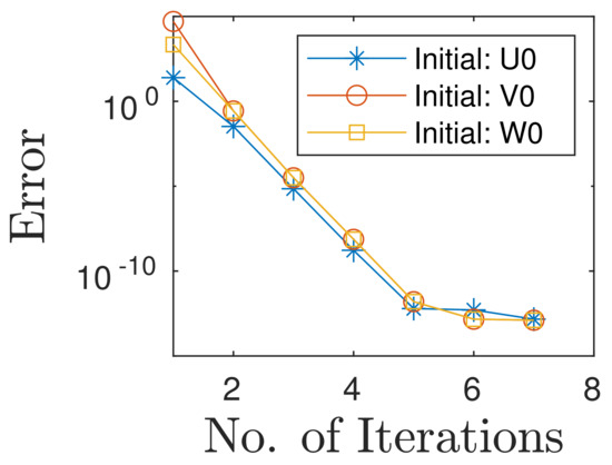
Figure 1.  Convergence behavior. 

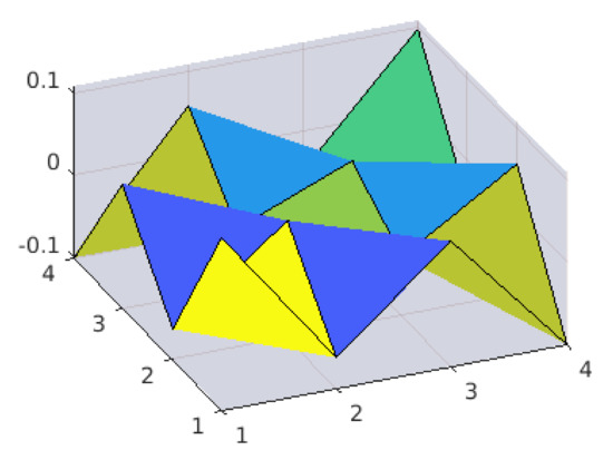
Figure 2.  Surface plot.

References

- Ran, A.C.M.; Reurings, M.C.B. On the matrix equation X + A*F(X)A = Q: Solutions and perturbation theory. Linear Algebr. Appl. 2002, 346, 15–26. [Google Scholar] [CrossRef] [Green Version]
- Ran, A.C.M.; Reurings, M.C.B. A fixed point theorem in partially ordered sets and some applications to matrix equations. Proc. Am. Math. Soc. 2004, 132, 1435–1443. [Google Scholar] [CrossRef]
- Turinici, M. Fixed points for monotone iteratively local contractions. Demonstr. Math. 1986, 19, 171–180. [Google Scholar]
- Nieto, J.J.; López, R.R. Contractive mapping theorems in partially ordered sets and applications to ordinary differential equations. Order 2005, 22, 223–239. [Google Scholar] [CrossRef]
- Nieto, J.J.; López, R.R. Fixed point theorems in ordered abstract spaces. Proc. Am. Math. Soc. 2007, 135, 2505–2517. [Google Scholar] [CrossRef]
- Kanel-Belov, A.; Malev, S.; Rowen, L.; Yavich, R. Evaluations of noncommutative polynomials on algebras: Methods and problems, and the Lvov-Kaplansky conjecture. SIGMA Symmetry Integr. Geom. Methods Appl. 2020, 16, 61. (In English) [Google Scholar] [CrossRef]
- Abbas, M.; Parvaneh, V.; Razani, A. Periodic points of T-Ćirić generalized contraction mappings in ordered metric spaces. Georgian Math. J. 2012, 19, 597–610. [Google Scholar] [CrossRef]
- Samet, B.; Turinici, M. Fixed point theorems on a metric space endowed with an arbitrary binary relation and applications. Commun. Math. Anal. 2012, 13, 82–97. [Google Scholar]
- Ahmadullah, M.; Ali, J.; Imdad, M. Unified relation-theoretic metrical fixed point theorems under an implicit contractive condition with an application. Fixed Point Theory Appl. 2016, 2016, 42. [Google Scholar] [CrossRef] [Green Version]
- Ahmadullah, M.; Imdad, M. Unified relation-theoretic fixed point results via FR-Suzuki-contractions with an application. Fixed Point Theory Appl. 2020, 21, 19–34. [Google Scholar] [CrossRef]
- Ahmadullah, M.; Imdad, M.; Arif, M. Relation-theoretic metrical coincidence and common fixed point theorems under nonlinear contractions. Appl. Gen. Topol. 2018, 19, 65–84. [Google Scholar] [CrossRef] [Green Version]
- Ahmadullah, M.; Imdad, M.; Arif, M. Common fixed point theorems under an implicit contractive condition on metric spaces endowed with an arbitrary binary relation and an application. Asian Eur. J. Math. 2021, 14, 2050146. [Google Scholar] [CrossRef] [Green Version]
- Alam, A.; Imdad, M. Relation-theoretic contraction principle. J. Fixed Point Theory Appl. 2015, 17, 693–702. [Google Scholar] [CrossRef]
- Suzuki, T. A generalized Banach contraction principle which characterizes metric completness. Proc. Am. Math. Soc. 2008, 136, 1861–1869. [Google Scholar] [CrossRef]
- Kolman, B.; Busby, R.C.; Ross, S. Discrete Mathematical Structures, 3rd ed.; PHI Pvt. Ltd.: New Delhi, India, 2000. [Google Scholar]
- Lipschutz, S. Schaum’s Outlines of Theory and Problems of Set Theory and Related Topics; McGraw-Hill: New York, NY, USA, 1964. [Google Scholar]
- Maddux, R.D. Relation algebras. In Studies in Logic and Foundations of Mathematics; Elsevier B.V.: Amsterdam, The Netherlands, 2006; p. 150. [Google Scholar]
- Haghi, R.H.; Rezapour, S.; Shahzad, N. Some fixed point generalizations are not real generalizations. Nonlinear Anal. 2011, 74, 1799–1803. [Google Scholar] [CrossRef]
- Aliouche, A.; Djoudi, A. Common fixed point theorems for mappings satisfying an implicit relation without decreasing assumption. Hacet. J. Math. Stat. 2007, 36, 11–18. [Google Scholar]
- Popa, V.; Mocanu, M. Altering distance and common fixed points under implicit relations. Hacet. J. Math. Stat. 2009, 38, 329–337. [Google Scholar]
Publisher’s Note: MDPI stays neutral with regard to jurisdictional claims in published maps and institutional affiliations. |
© 2021 by the authors. Licensee MDPI, Basel, Switzerland. This article is an open access article distributed under the terms and conditions of the Creative Commons Attribution (CC BY) license (https://creativecommons.org/licenses/by/4.0/).