1. Introduction
In recent years, widespread interest has arisen concerning the description and analysis of dynamic systems governed by growth curves, owing to the need to explain the evolution of a variety of phenomena in the most precise way possible. Some examples include the study of cell growth (stem cells, tumors, and tissue regeneration), the diffusion of innovations (social networks and the implementation of new technologies), or the exploitation of energy resources (production peaks and length of exploitation periods). In this regard, the latest rage is probably the study of the evolution of epidemics such as COVID-19, in which concepts such as contagion peaks, inflection points in the spread of disease, duration, and onset times of successive waves are of paramount importance for the purposes of planning and policy making. In all cases, the objective is to explain the behavior of the phenomenon and allow for its prediction while keeping in mind that certain external influences may affect its evolution.
The study of growth curves has taken two distinct directions: the unification and the generalization of models (Chakraborty et al. [
1]). Unification refers to the compact representation of different models through a single function, which allows for improved mathematical manageability. As for generalization, it refers to the process that starts from a simple equation to which parameters or functions are subsequently incorporated. Its goal is to generate more flexible forms and thus increase applicability to a wider range of research areas. Some outstanding examples of unification are the works of Martínez et al. [
2] and Tjørve [
3] which propose a variety of approaches for a growth equation that unifies many of the existing sigmoidal growth curves. As for generalization, we can cite the works of Tsoularis and Wallace [
4] and that of Koya and Goshu [
5]. Although generalized equations offer greater flexibility in form, the resulting models have a harder time of fitting real data sets on account of their complexity. For this reason, the idea of including new parameters has been recently combined with that of introducing flexible functions. In this sense, Tabatabai et al. [
6] have constructed the so-called hyperbolic curves and shown their usefulness in the study of the evolution of tumor processes and stem cell growth (Tabatabai et al. [
7]). Furthermore, and more precisely, such models have been used to describe the growth of the solid Ehrlich carcinoma under combined treatments (see in [
8]). To this end, all three hyperbolastic models are used and compared in different scenarios. Related to this, the type II is employed to model the dynamics of cervical cancer mortality rates [
9]. See also in [
10], where hyperbolastic curves are used to introduce a model of wound healing. All of these models are the starting point for the development of others, such as the oscillabolastic, which aim to model oscillatory growth (Eby and Tabatabai [
11]). Similarly, T-type models (Tabatabai et al. [
12]) are capable of representing biphasic sigmoidal growths characterized by stages of growth and decrease, that is, multisigmoidal patterns of behavior. Along these lines, Erto and Lepore [
13] have recently defined a new type of sigmoidal curve which, given that certain parametric conditions are met, presents more than one inflection point.
As the variability of the phenomena under study cannot be controlled in deterministic models associated with growth curves, randomness is included in the ordinary differential equations from which they originate. To this end, we employ stochastic differential equations whose solutions are, under certain conditions, diffusion processes. The most widely studied curves in this context are, without a doubt, the logistic and Gompertz curves. For example, Schurz [
14] considered a fairly general version of the stochastic differential equation associated with logistic growth, and Rupšys [
15] introduced several versions of the differential equation that included delays, whereas Schlomann [
16] studied logistic diffusion processes in the presence of catastrophes. This field is unceasingly producing new research, as exemplified by the recent works of Rajasekar et al. [
17,
18] in which the authors analyzed a stochastic version of the SIR models for the spread of the COVID-19 pandemic. On the other hand, the fact that the Gompertz curve is an excellent model for the description of tumor growth has motivated the introduction of several diffusion processes associated with it (see, for example, Lo [
19] and Ferrante [
20]). On the basis of these processes, various modifications have subsequently been made with the goal of describing the evolution of tumor growth in the presence of therapeutic treatments (Albano et al. [
21,
22,
23]).
With regard to diffusion processes associated with other growth curves, the existing references are scarce. Perhaps the main difficulty lies in the fact that, although the stochastic differential equation may have a solution (and sometimes not in a totally explicit way), the diffusion process obtained therefrom is not totally manageable. This is a problem even in the logistic case. Skiadas [
24] presented an exact solution for the logistic stochastic differential equation with multiplicative noise, although its shape showed that some characteristics cannot possibly be obtained in an explicit fashion, as is the case of transition probability density functions. Therefore, when studying this process one must resort to the discretization of the differential equation. However, convenient reformulations of some growth curves have succeeded in verifying a differential equation of the Malthusian type, which is the way to construct diffusion processes based on modifications of the inhomogeneous lognormal process. Such modeling allows for diffusion processes with transition densities whose functional form is perfectly known. Such is the case of the Bertalanffy (Román-Román et al. [
25]), Richards (Román-Román and Torres-Ruiz [
26]), and Hubbert curves (Luz Sant’Ana et al. [
27]). An alternative way is the modification of ordinary differential equations verified by certain growth curves, which can be done by including in them certain temporal functions. Thus, from the logistic and Weibull equations, Barrera et al. [
28,
29] introduced the hyperbolastic diffusion processes of type I and III. Likewise, and following this same idea, a multisigmoidal stochastic version of the logistic process has been obtained (Di Crescenzo et al. [
30]) as well as a diffusion processes linked to the oscillabolastic curve (Barrera et al. [
31]).
The main aim of this paper is to present a common model for diffusion processes associated with the family of hyperbolastic curves. Our proposal not only allows for the results obtained for the type I and type III models to be unified, but also extends them to the hyperbolastic curve of type II. The present paper is structured as follows.
Section 2 makes a brief summary of the family of hyperbolastic curves. Additionally, and with the definition given by Tabatabai et al. in [
6] as a starting point, it is verified how each of the curves satisfies an ordinary differential equation of the Malthusian type, which extends the deterministic models to stochastic ones that have the non-homogeneous lognormal diffusion process as common point, this being the objective of
Section 3. Furthermore, and given that these models are appropriate to describe real phenomena governed by hyperbolastic curves, the inference in them must be developed.
Section 4 describes a unified version for the three models presented. Of particular interest is the description of how initial solutions are obtained for the resulting system of maximum likelihood equations. Note that this joint vision enables an efficient computational implementation of the procedures derived from the inferential development herein described. Finally,
Section 5 presents some simulation-based examples.
2. An Overview of Hyperbolastic Growth Curves
For the sake of clarity, this section will provide a brief summary of the hyperbolastic curves to date. One of the most interesting aspects of the following description is the fact that all three hyperbolastic models can be seen from a unified perspective.
The hyperbolastic model of type I (
) appears as an extension of the classic logistic model in which a certain hyperbolic function is introduced. Concretely, the
curve is the solution of the initial value problem
resulting in
where
. Here,
M represents the carrying capacity of the system under consideration whereas real parameters
and
jointly determine growth rate. We note that parameter
gives the intrinsic growth rate, whereas
controls the distance from the
curve to the logistic one. Regarding function
, it will play an important role in the unification of the strategies required to work with this and similar models, as it encodes the action of the temporal function that distinguishes models I and III, and which also characterizes the type-II model. Another interesting aspect is the value of the asymptote. As it is verified that
, then
if
, and
if
. In any case, the value of
M is independent from the initial value, which can significantly restrict some applications. In practice, there are situations in which the growth phenomenon under study shows an
-type sigmoidal growth and several sample paths are available, each with the same growth pattern but with different initial values and upper bounds. This can be avoided by re-parameterizing the curve. Indeed, after replacing
with a new parameter
, and
M with
, expression (
2) becomes
for which it is verified that
. Here,
represents parametric vector
. This last reformulation of the model allows us to describe trajectories with different values of asymptotic stabilization in terms of the initial state
.
Regarding the hyperbolastic curve of type II (
), its introduction presents an increase in complexity with respect to the type-I model. This curve is defined as
being the solution of the ordinary differential equation
with initial condition
. Here,
, parameters
M,
, and
can take any real value and
In this case,
represents the intrinsic growth rate whereas
is an allometric constant. Note also that (
3) tends to
M when
, and to extinction (
) when
. This leads
to assume a key property in the dynamic evolution of the model. Again, this goes to show how the limit value does not depend on the initial condition. By applying the same reasoning as in the previous case, we arrive at the following reformulation of curve
verifying that
, being now
.
Finally, the hyperbolastic model of type III (
) follows the structure established for the
curve, but this time using the classic Weibull ordinary differential equation as a starting point. In this way, the
ordinary differential equation arises, resulting in
Considering
, the solution of (
4) is
being
. The real parameters
and
are an intrinsic growth rate and an allometric value, respectively, whereas
represents the distance from the
curve to the classical Weibull model. By applying to the limit value of the curve a reasoning analogous to the ones described above, we arrive at the following reformulation of the curve
for which it is verified that
.
As it has been shown, each of the hyperbolastic curves is the solution to a certain ordinary differential equation. However, it is not difficult to verify that each curve also verifies a Malthusian-type differential equation. Specifically, one has
where
, being
the Kronecker delta and
Note that the functions do not depend on the initial values taken by the curves. This unified formulation allows us to extend the hyperbolastic deterministic procedure to stochastic versions under the prism of the inhomogeneous lognormal diffusion process, which is the objective of the next section.
Finally, note that an important characteristic of this type of sigmoidal models is the presence of inflection points, as well as the expressions that they must verify. Note that the number of inflections generally increases the flexibility of the curve and its adaptation to a variety of observations. From (
5), the inflection time instants are the solutions of the equation
In general, the resulting equations are quite complex and in practical cases strategies for their estimation will be developed from the observed data. On the other hand, such an expression will allow us to integrate a procedure for calculating initial solutions for the different parameters, as we will see in later sections.
3. Hyperbolastic Diffusion Processes
The deterministic hyperbolastic models presented in the previous section enable the description of growth phenomena in contexts in which detailed knowledge of their leading variables exists. However, such models do not account for the effects of external factors influencing the development of phenomena. For this reason, we must address the development of stochastic models which, while based on the previous ones, attempt to overcome their shortcomings.
Such models are commonly built by adding a multiplicative noise to the original ordinary differential equations. The multiplicative noise is considered more suitable than the additive one in the context of growth phenomena. Thus, random influences are made dependent on the state of the system at each instant.
However, this methodology can lead to stochastic differential equations whose solution is not easy to handle, mainly due to lack of explicit characteristics such as transition densities, which may affect practical applications. For example, consider the case of the
hyperbolastic model. From (
1) we consider the stochastic differential equation
where
represents the standard Wiener process, independent of initial condition
for
, being
the volatility parameter.
This equation can be solved by using the following integrating factor (see [
32])
from which the solution can be expressed as
where
.
Note that, although the stochastic differential equation can be solved, the form of the solution does not provide an explicit distribution of , which renders the analytic treatment of the process difficult. In fact, to this purpose the literature discretizes the stochastic equation and obtains numerical approximations. This is the rationale behind the next subsection, in which we will consider stochastic, more manageable versions of the models.
Hyperbolastic Diffusion Processes from the Non-Homogeneous Lognormal Diffusion Process
Based on the previous comments, this section proposes the construction of hyperbolastic stochastic models which are analytically manageable and in which the mean of the process can be associated with the original curve. To this end, we will employ the lognormal process with exogenous factors, which has the aforementioned properties and allows us to work extensively with the resulting diffusions. As is known, the inhomogeneous lognormal process is built on the basis of a differential equation of the Malthusian type with a time-dependent growth rate, to which a multiplicative noise is added as described above (see Roman et al. [
33]). Therefore, and given that the hyperbolic curves all verify a Malthusian-type differential equation, it is therefore possible to associate each of them with an inhomogeneous lognormal diffusion process whose mean is precisely the curve in question. In addition, the properties of this type of process make it perfectly treatable, since its finite-dimensional distributions are explicitly available.
Briefly, the non-homogeneous lognormal diffusion process (or with exogenous factors) is the solution to the linear stochastic differential equation
with initial condition
.
is a continuous function depending on a vectorial parameter
whereas
is the standard Wiener process, independent of
for
. The solution of this equation is
where
Indeed, if
, then, by Itô’s formula, it follows that
which leads to a Gaussian process
Z, with
X then being lognormal.
Given its Markovian character, the distribution of the process follows from that of
. Indeed, if
is a lognormal distribution
, or
is degenerate at a value
(
a.s.), it can be shown that the finite-dimensional distributions of the process follow a lognormal distribution. Specifically, vector
, for
with
, follows a
n-dimensional lognormal distribution
where the components of vector
and matrix
are
and
respectively. In particular, from the two-dimensional distributions
it follows that
so the transition probability density function takes the form
Regarding the main characteristics of the process, we highlight the moments of order
n, whose expression is
From this expression, it is evident that for a convenient choice of function allows many types of curves to be modeled by this process.
Note that by using this methodology in the construction of the processes, certain issues are addressed which could not be if the classical method of introducing a multiplicative noise in the original deterministic differential equation had been followed. Ultimately, we must not forget that our goal is to model phenomena which exhibit behaviors that are governed by these types of curves.
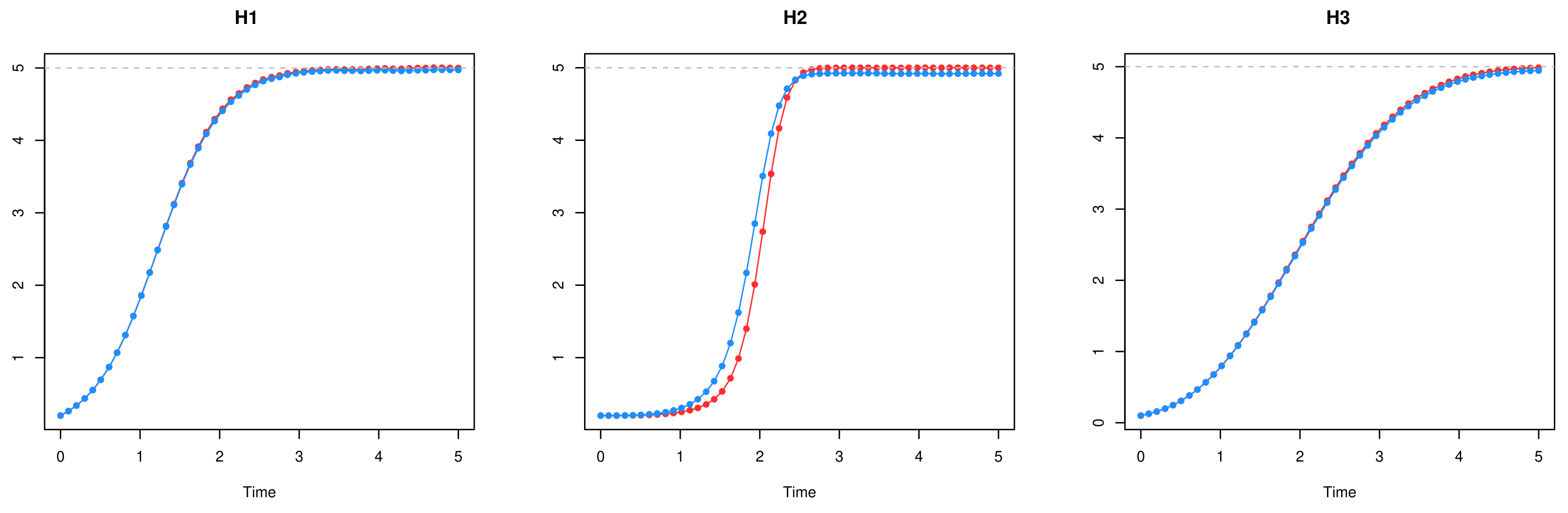
Figure 1 shows, for each hyperbolastic process, a comparative graph of the means obtained from simulated trajectories using each stochastic differential equation (the original and the Malthusian). This illustrates how the behavior is the same in both cases.
4. Inference
As shown above, one of the main strength of the models presented here is their flexibility, which makes them suitable for describing and fitting growth patterns in real cases.
There are, at least, two natural ways to identify the parameters in our stochastic hyperbolastic models. The first is the direct use of likelihood methods, and the second is particle filtering (PF). Herein, we will employ the former due to its widespread use. However, we also want to point out that our unification and linearization work applies equally well to PF (see, e.g., in [
34,
35]). In this method, the lognormality assumption on
is not required. The parameters to be identified would become the
signal (with trivial dynamics) and the logarithm of the linearized hyperbolastic SDEs would become the classical observations. Finally, one could use PF on the non-linearized SDEs, which would require a little manipulation of the observation function coming from the integrating factor solution (shown in
Section 3 for the type-I case).
Despite the above, in this section we address the estimation of the parameters of the model by means of the maximum likelihood (ML) method. However, it must be taken into account that the functional and parametric complexity of the models makes the estimation procedure remarkably difficult. In order to tackle this issue, the estimation by maximum likelihood will require the use of numerical procedures, many of which will demand the computation of initial solutions for the parameters.
4.1. Maximum Likelihood Equations
The starting point for the estimation procedure is the observation of d sample-paths at time instants , . Note that neither the sample sizes nor the times of observation have to be the same. Moreover, we will suppose that , for all . Let be the vector containing the random variables of the i-th sample-path, that is , , and denote . Furthermore, we will consider that follows a lognormal distribution, concretely (as it has been said before, this would not be a requirement if the particle filtering approach were to be used).
From (
8), and considering a fixed value
of
, the log-likelihood function for each model, defined in a unified way for
, is
where
,
is the parametric vector of the initial distribution, and
being
. The expression of function
will depend on the hyperbolastic case under study. Nevertheless, it is possible to find a unified formulation by considering
, where
with
and
Under the assumption that
and
are functionally independent, the estimate of
is
while that of
is obtained (see [
33] for details) from the system of equations
where the grouped variables are defined as follows:
The partial derivatives of are calculated with respect to the parameters of every model, and therefore they depend on ℓ. Indeed, these parameters involve a common one, say , as well as the particular ones of each model: for the model, for the model, and in the case of the model.
All these expressions can be unified as follows:
where
and
.
Despite the few parameters involved, this system remains too complex to be solved with analytical methods. Therefore, numerical methods, such as the Newton–Raphson procedure, are the proper way to solve the system. Nevertheless, initial solutions for the parameters are required in order to apply such methods. In this case, such solutions can be obtained from the information provided by the data and taking into account the properties of the curve.
4.2. Initial Solutions
As we mentioned before, solving the system of Equation (
10) by means of numerical methods requires finding initial solutions first. This task may prove daunting according to the degree of complexity of the hyperbolastic models. In this section, strategies for the search of initial solutions are proposed for each hyperbolastic stochastic model.
The vector of parameters to be estimated is , where comprises and the rest of the parameters of the model under study. All of these parameters are related within the expressions derived from each model, and therefore the initial value of one parameter may depend on the initial value of another. A strategy is then required which will provide a sequence of steps that guarantee the final computation of all values.
As shown in
Section 2, type-I and -II models have two parameters each, besides parameter
, which is common to both, and diffusion parameter
. On the other hand, type-III models have three parameters:
, and
. This model will require a particular step in the procedure. We propose the following search schema.
Initial solution for
: it is known that, for a lognormal distribution
, an estimation of
is provided by the quotient between the arithmetic and geometric means. By taking advantage of this result, the initial value of
, in the case of a degenerate initial variable
, is obtained by linear regression of
against
, for
. Here,
and
are, respectively, the arithmetic mean and the geometric mean of the sample paths at time instant
. If
is not degenerate, i.e.,
, then
provides an estimate of
for each
, thus a previous estimation of
is required. This can be accomplished from the values of the sample paths at the first observation time
by using (
9).
Initial solution for the rest of the parameters: the general procedure involves considering the two parameters at once (in the type-III model, one of the parameters must be fixed) and using expressions derived from the curve. Indeed, we can see how, for each of the reformulations made for the curves, parameter
can be expressed as a function of the rest of the parameters and the limit value of the curve. Then
can be viewed as a function
of the parameters of every curve. Note that this can be accomplished because
for all
. The expressions for every model are then
where
, and
are the limit values of every curve, respectively. Given that these values are, as a general rule, not known, an approximation that uses the last values of the mean observed data can be considered.
The goal then is to use the information provided by the observed inflection time of the curve. Let
be an inflection time instant, which can be obtained by fitting a spline function to the observed mean values and finding either the maximum of its first derivative or a zero value of its second derivative. Note that
must verify Equation (
6). This fact will allow us to obtain the initial values of the rest of the parameters. To this end, we define function
Here, notation
alludes to the fact that we have substituted functions
in the expressions of functions
, so that function
I depends only on the parameters of interest. Finally, the selected values will be those that minimize function
I in a bounded region. In particular, candidates can be obtained from such bounded region satisfying the condition
where
is a prescribed error threshold. We recommend varying its order of magnitude between 0.0001 and 0.1, depending on the sample data. At this step, and in order to achieve a good implementation, it is worth differentiating the following cases:
- (a)
Type-I and -II models: initial values for pairs of parameters (model I) and (model II) can be obtained by applying the aforementioned methodology where the bounded regions are two-dimensional in every case. The limits of such regions can be proposed following the nature of the parameters. and are growth parameters in their respective models, so their magnitude would be related with the observed growth. On the other side, is the “distance” to the logistic curve and an allometric constant, and therefore their bounds can also be proposed according to the phenomena observed.
- (b)
Type-III model: there are three parameters in vector . In order to avoid a three-dimensional region, we propose fixing parameter provided that is the “distance” to the Weibull curve. That is, by fitting a Weibull model to the observed data, an estimate of could be considered the initial value of the parameter. Next, the methodology described above could be applied for the pair . Simulation studies may be carried out in order to verify the stability of the solutions according to fluctuations in the fixed value of . On the other hand, considerations about the bounded region are then the same as in the other two models.
Initial solution for : once solutions for the other parameters have been obtained, an initial value of follows from applying to such initial values. As it has been said, limiting values can be obtained by taking the last value of the observed mean data. Nevertheless, if , then for all , and the initial value of is independent of the rest of the parameters.
5. Simulation
In this section, the proposed methodology is applied to simulated data. For the three hyperbolastic models, a simulation study is carried out concerning the variability of the diffusion parameter, named
, and the number
n of observations. For every model, 20 sample paths were simulated with the same final time instant at
and time step
. Thus, 501 points for each path were simulated in every iteration. In all three cases, an initial degenerate distribution at
were considered, in the sense
. Furthermore, three different diffusion coefficient values were used in every simulation, being
and
. Then, three subsets of equidistant points were extracted according to values
and 51. There were, therefore, 9 sets of data for combinations of
n and
. In every case, 100 replications were carried out. In every one of these, the sample paths were simulated following (
7) and the proposed methodology was applied. In particular, initial solutions were considered according to
Section 4.2. Then, the corresponding system of ML equations was solved following
Section 4.1. In order to obtain good performance and improved results, after every replication the mean value between the current solution and the mean of the solutions from previous iterations were computed. The particular parameters for every hyperbolastic models were:
for the model: ,
for the model: ,
for the model: .
Finally, the relative absolute error (RAE) from the observed mean to a new simulated mean with estimated parameters was computed. The expression for RAE is done by
where
is the mean observed value at time
,
is the mean value of the estimated process at time
, and
n is the sample size.
A total number of 2700 computations were performed. All of them were performed in R. The solutions of ML equations were obtained with the packages “nleqslv” [
36] and “BB” [
37].
Results are shown in the following tables for initial and final solutions. In the latter case, an additional column showing the RAE has been included.
After a more in-depth analysis, it is shown that the RAE is low in all the three hyperbolastic models. Note that this error measures the difference between the observed mean and the mean of a new diffusion process simulated with the estimated parameters. Furthermore, with being the parameter concerning the variability of the paths, it is expected that the error growths as does. Nevertheless, the combination with different sample sizes (n) can lead to particular behaviors for each hyperbolastic model.
In the case of the
model,
Table 1 shows that the RAE increases with
and, for every value of this parameter, it remains approximately the same for all sizes
n. This leads to the conclusion that the
model behaves well regardless of sample size. Let us remember that such model can be viewed as an extension of the classic logistic growth model. Furthermore, such invariant behavior for different values of
n could be expected seeing the contents of
Table 2, which shows that initial values for parameters
and
are exactly the same for every
n. In the case of
, they are also the same for all
.
Figure 2 shows a comparison between the observed sample mean and the mean of the simulated new process after extracting the corresponding number of equidistant points. It can be seen that the fitness of the model is good, even when variability is high. For that case, the last row of figures shows a slight growing deviation from the observed mean. Nevertheless, the overall behavior of the model is appropriate. On the other hand, the evolution of RAE alongside
and independently of
n for the
model can be observed clearly in the corresponding table. As an addition to this, and in order to illustrate the procedure, graphs related with the search of initial values for the
model in the last combination, corresponding to
and
, are shown in
Figure 3. Following the methodology proposed in
Section 4.2, a search for initial solutions
and
had been performed in square
divided into 100 points at every dimension, amounting to
points in the whole region. At every pair of points, the inflection function derived from (
6) was tested for an error
. The histograms for all suitable values of
and
are shown in
Figure 3, respectively, as well as red lines at the selected values (the median). Furthermore, a plot showing levels of the inflection condition function is shown in the last image. The region at which the error is below of
is filled in blue. Finally, red lines from final
and
are crossed at each selected pair.
The final results for the model
are shown in
Table 3. They shown the expected behavior, with an increment of the error proportional to that of related with
. Nevertheless, this model exhibits the lower error among the three hyperbolastics. Initial solutions
and
(see
Table 4) were found in a region
, where bounds for
are chosen according to the fact that it appears as the exponent of time, that is,
, in the expression of the
model. The comparisons between observed and estimated mean values for every combination are shown in
Figure 4, where the influence of
can be observed in the variability of observed values. Such influence is particularly noticeable in this example because the curve reaches its limit behavior earlier than in other models. This implies that more observations are therefore subject to growing variability. Even in that case, the estimated mean points are a good fit for the observed ones, for all
and all
n.
Finally, estimated values and initial solutions for the
model are shown in
Table 5 and
Table 6, respectively. According to the former, it can be observed that errors (RAE) follow the same pattern for every value of
and their combination with
n. Indeed, the estimated values lead to the same errors for all
. The reduction of the error in this model appears when
n increases, as expected, but being more noticeable that in the other models. In any case, RAE remains practically the same for all combinations. On the other side, initial values of
and
are the same when
n is varying. In the case of the
model, the search region for initial values
and
was the rectangle
. The initial value
was obtained, in every combination, after fitting a Weibull curve to the observed mean by nonlinear least squares (a study of the stability of such approach concerning
was carried out in [
29]). This behavior is illustrated by
Figure 5. In particular, the most noticeable differences between observed and estimated mean points appear for low values of
. When variability increases the model appears to behave better, showing that it would be suitable to describe complex growth dynamics with a high degree of variability.
A comparison between the results of the three models shows that the lowest RAE is achieved with the hyperbolastic model of type II. The type-I model also yields low RAE values, but mainly for low variability. The type-III model is the one showing the highest RAE for . Despite such error being higher than in the other two models for high values of , it remains stable and does not vary too much. The first conclusion to be drawn from this comparison is that the type-II model displays the best behavior, but the type-III model seems to be more flexible as it can be more successfully adapted to a variety of scenarios.
6. Conclusions
Associated with each of the hyperbolastic functions (, , ), a stochastic model has been presented based on a diffusion process whose mean function is the curve under consideration. A previous analysis of the hyperbolastic curves determines that all of them can be considered as the solution of a linear ordinary differential equation, more specifically of the Malthusian type. This provides a joint vision of all the curves and allows us to extend the deterministic models to stochastic ones, which is done through stochastic differential equations obtained by adding a multiplicative noise to the previously mentioned Malthusian equation. Thanks to this unification of models, global inference procedures can be presented for all of them, which include both obtaining the system of maximum likelihood equations and describing the common procedure by which the initial solutions required to solve said system are obtained. This unified perspective is particularly useful in simplifying the computational implementation of numerical procedures to fit data from real phenomena.
A simulation study has been carried out concerning initial and final solutions for different combinations of variability and sample size. Results show that every model behaves as expected but with subtle differences according to the combination of and n. As a matter of fact, the type-I model is affected by increasing variability, with this being higher as the sample size increases. The type-II model shows the lower errors and, finally, the error in the case of the type-III model remains the same for every combination of variability and sample size, and its reduction with n becomes more noticeable than in other models.
Future research lines might concern the inclusion of the processes herein described in richer models able to describe more complex behaviors. Indeed, hyperbolastic growth models could be useful in addressing random growth in several other models (e.g., epidemiological models such as SIR or SEIR, or any other describing biological phenomena such as tumor growth or tumor suppression). To this end, it must be noted that the power of hyperbolastic models, as is the case of many others, relies mainly on their number of parameters as well as the flexibility of their intrinsic functions. This implies a growing, data-dependent complexity in the estimation of parameters and the performance of other statistical procedures. This limitation must be acknowledged and considered in order to build reliable models.


