A Solution of Richards’ Equation by Generalized Finite Differences for Stationary Flow in a Dam

Abstract

The accurate description of the flow of water in porous media is of the greatest importance due to its numerous applications in several areas (groundwater, soil mechanics, etc.). The nonlinear Richards equation is often used as the governing equation that describes this phenomenon and a large number of research studies aimed to solve it numerically. However, due to the nonlinearity of the constitutive expressions for permeability, it remains a challenging modeling problem. In this paper, the stationary form of Richards’ equation used in saturated soils is solved by two numerical methods: generalized finite differences, an emerging method that has been successfully applied to the transient case, and a finite element method, for benchmarking. The nonlinearity of the solution in both cases is handled using a Newtonian iteration. The comparative results show that a generalized finite difference iteration yields satisfactory results in a standard test problem with a singularity at the boundary.

1. Introduction

Water flow is one of the most relevant phenomena in geotechnical engineering because it modifies the mechanical properties of the soil. In the field of civil engineering, there are many structures where the soil is used as a construction material; among the most important ones are dams and embankments. They are subject to environmental effects since the water enters into structures that are subject to the environment and eventually modify its mechanical behavior. Among the catastrophic events that can be caused by infiltration processes are sinkhole collapses, Ref. [1], and landslides [2,3].

To describe the dynamic mentioned above, Richards’ equation is adopted [4]. It is a degenerate elliptic–parabolic equation and is considered an adequate formulation of the problems since it takes into account the unsaturated condition of the soil in a realistic way. Although, an accurate numerical formulation requires an adequate discretization of the strong nonlinear relation between the pressure head, the water content, and the hydraulic conductivity. This nonlinearity must be included both in the temporal and spatial discretizations.

The numerical problem must be addressed from two points of view: the discretization of the differential equation and the solution of the discrete system. This paper aims to address the discretization of Richards’ equation. Due to its importance and its wide range of applications, several authors have solved it using different techniques, such as the Finite Element Method (FEM), the Finite Volume Method (FV) and the Finite Differences Method (FD).Extensive reviews on the subject have been conducted, among other authors, by Zha et al. [5], Farthing and Ogden [6], and List and Radu [7]. Nevertheless, despite the intensive research conducted in recent decades, there is still a strong need for robust numerical schemes for multiphase flow in porous media.

FEM has been widely used and is a standard reference method for benchmarking due to many studies where successful results were obtained in one-, two-, and three-dimensional problems [8,9,10,11,12,13,14,15]. However, in some transient problems, the numerical results for infiltration were found to exhibit strong oscillations, a phenomenon that has been associated with the mass matrix in the formulation [8].

The finite volume has been used to solve Richards’ equation in one [15,16,17,18,19] and two spatial dimensions [17,20]. One of the advantageous features of the finite volume method is that water balance is taken into account in the scheme at every time step since it is calculated at the borders of a control volume as a part of the algorithm, implementing the mass-conservative iterations straightforwardly [17,18]. Another advantage is that the method has applicability in unstructured meshes, which endows it with flexibility [17,21].

In the case of finite differences, most of the papers analyze the one-dimensional problem [8,22,23,24,25] to assess the accuracy, stability, and convergence of the method [21]. One of its main limitations is the lack of schemes in irregular domains because the stencils developed for structured meshes could not be used in 2D complex domains with unstructured grids. Nevertheless, some interesting adaptations were proposed, such as that of Hsieh [26], which was designed for block-rectangular domains.

Differences in block domains and symmetric nonrectangular domains prepared the way for more general schemes. Nowadays, there are new formulations of finite differences that can be applied to complex domains with structured and unstructured meshes. In recent times, the Generalized Finite Differences Method (GFDM) [27,28], which is an extended case of the classic finite differences, has shown to be especially useful for irregular boundaries without losing the simplicity of the traditional method. The method has shown the capabilities to numerically solve the transient differential equations which describe water flow in complex boundaries with structured grids [29,30,31,32]. The simplicity behind the formulation of the GFDM is one of its main advantages. In this case, the idea is to obtain weights for each node, as a function of the relative distance of the surrounding nodes to a central point using the Taylor expansion. This yields a method that can even be applied as a meshless one, because a specific grid structure is not required to assign the weights. For instance, in Milewski’s work [33], an unstructured, arbitrarily distributed cloud of nodes is used, as well as an ad hoc node selection, to produce accurate results. Certainly, generalized finite differences can also be applied to structured meshes and irregular domains [27], which has an advantage over the meshless methods that the grid structure for the calculation of the coefficients uses.

Due to this reason, the GFDM has also been used for solving parabolic and elliptic partial differential equations successfully. In the present work, the GFDM is tested against FEM to solve Richards’ equation in stationary formulation for a dam case with boundary singularities [34]. This form of the Richards’ equation is an elliptical PDE with highly nonlinear constitutive relations. The hydraulic conductivity $k(\theta )$ and suction $s(\theta )$ functions have nearly zero values that can produce a degenerate form of the equation [6], which makes the problem especially complex due to the dependence of the hydraulic permeability on the solution, so a Newton–Raphson (NR) iteration needs to be applied to solve the nonlinear discrete problem.

This paper is organized as follows: Section 1 presents the introduction to the problem. The materials and methods are discussed in Section 2 and the results and discussion are addressed in Section 3. Finally, the conclusions are presented in Section 4.

2. Materials and Methods

2.1. Richards’ Equation

Richards’ equation [4] for the case of the stationary condition in two dimensions can be written as [35]

$$\frac{\partial }{\partial x}\left(k_x\frac{\partial h_w}{\partial x}\right)+\frac{\partial }{\partial y}\left(k_y\frac{\partial h_w}{\partial y}\right)=0$$

(1)

where:

$h_w=y+\frac{u_w}{{\gamma }_w}$ is the total hydraulic head;

y is the gravitational head;

$u_w$ is the pore water pressure;

${\gamma }_w$ is the unit weight of water;

$k_x(s)$ and $k_y(s)$ are the water permeability coefficients along the x- and y-axis;

$s=u_a-u_w$ is the matrix suction relative to the reference air pressure $u_a$, which was set as equal to zero in this paper.

In this formulation, the cornerstone to produce realistic results is an adequate definition of the permeability coefficients. Under isotropy considerations, the same coefficient k can be used in both coordinate directions. The van Genuchten–Mualem equation [36], which can be written as

$$k({\theta }_n)=k_s\sqrt{{\theta }_n}{(1-{({\theta }_n^{1/m})}^m)}^2,$$

(2)

is often used for that purpose. Here:

${\theta }_n=\frac{{\theta }_w-{\theta }_r}{{\theta }_s-{\theta }_r}$ is the normalized volumetric water content;

${\theta }_w$ is the actual volumetric water content;

${\theta }_r$ is the residual volumetric water content;

${\theta }_s$ is the saturated volumetric water content;

$n,m$ are fitting parameters, related as $m=1-\frac{1}{n}$.

On the other hand, the normalized volumetric water content ${\theta }_n$ can be represented by the following equation proposed by van Genuchten [37]

$${\theta }_n(s)=\frac{1}{{\left({(\alpha s)}^n+1\right)}^m}$$

(3)

where m and n are the fitting parameters defined in Equation (2).

2.2. Finite Difference Formulation

Under smoothness assumptions, Richards’ Equation (1) can be written in a differential form as follows

$$k_x\frac{{\partial }^2{h}_w}{\partial x^2}+k_y\frac{{\partial }^2{h}_w}{\partial y^2}+\frac{\partial k_x}{\partial x}\frac{\partial h_w}{\partial x}+\frac{\partial k_y}{\partial y}\frac{\partial h_w}{\partial y}=0.$$

(4)

For this work, bearing in mind its successful application to solve an unsteady Richards equation [28], the formulation of generalized finite differences is used to approximate the solution of the Equation (4).

The procedure to approximate differential operators using generalized finite differences for nonrectangular regions considers a linear combination of the values of the function $h_w$ at a finite set of nodes $p_0=(x_0,y_0), p_1=(x_1,y_1), p_2=(x_2,y_2),\dots , p_k=(x_k,y_k)$ in such a way that the local consistency condition is fulfilled. Thus, the truncation error at $\tau (p_0)$

$$\tau (p_0)=L(h_w,A(x,y),B(x,y),C(x,y),D(x,y),E(x,y))-{\displaystyle \sum _{i=0}^q}{\mathsf{\Gamma }}_i{h}_w(p_i)$$

(5)

is used to define a second-order approximation to the linear operator

$$\begin{array}{ccc}L(h_w,A(x,y),B(x,y),C(x,y),D(x,y),E(x,y))& =& \\ A(x,y)\frac{{\partial }^2{h}_w}{\partial x^2}+B(x,y)\frac{{\partial }^2{h}_w}{\partial y^2}+C(x,y)\frac{\partial h_w}{\partial x}+D(x,y)\frac{\partial h_w}{\partial y}& +& E(x,y)h_w\end{array}$$

(6)

at the point $p_0$. Here, the values ${\mathsf{\Gamma }}_i, i=1,\dots ,q$, are the weights in the generalized finite difference scheme, and the functions $A(x,y)$, $B(x,y)$, $C(x,y)$, $D(x,y)$ and $E(x,y)$ are coordinate dependent functions which define the second-order operator L in Equation (6). The approximation sought is given by the second term on the right-hand side of the Equation (5), which is a linear combination of $h_w$, evaluated at $p_0, p_1,\dots ,p_k$, while the first term is the evaluation of the operator L in the central node $p_0$. Consistency implies that the coefficients ${\mathsf{\Gamma }}_l$ can be obtained from the Taylor expansion of Equation (5) at $p_0$ by imposing the following conditions

$$\left(\begin{array}{ccccc}\hfill 1& \hfill & \hfill 1& \hfill \dots & \hfill 1\\ \hfill 0& \hfill & \hfill \mathsf{\Delta }{x}_1& \hfill \dots & \hfill \mathsf{\Delta }{x}_q\\ \hfill 0& \hfill & \hfill \mathsf{\Delta }{z}_1& \hfill \dots & \hfill \mathsf{\Delta }{z}_q\\ \hfill 0& \hfill & \hfill {(\mathsf{\Delta }{x}_1)}^2& \hfill \dots & \hfill {(\mathsf{\Delta }{x}_q)}^2\\ \hfill 0& \hfill & \hfill \mathsf{\Delta }{x}_1\mathsf{\Delta }{z}_1& \hfill \dots & \hfill \mathsf{\Delta }{x}_q\mathsf{\Delta }{z}_q\\ \hfill 0& \hfill & \hfill {(\mathsf{\Delta }{z}_1)}^2& \hfill \dots & \hfill {(\mathsf{\Delta }{z}_q)}^2\end{array}\right)\left(\begin{array}{c}{\mathsf{\Gamma }}_0\hfill \\ {\mathsf{\Gamma }}_1\hfill \\ {\mathsf{\Gamma }}_2\hfill \\ .\hfill \\ .\hfill \\ .\hfill \\ {\mathsf{\Gamma }}_q\hfill \end{array}\right)=\left(\begin{array}{c}\hfill E(x_0,z_0)\\ \hfill C(x_0,z_0)\\ \hfill D(x_0,z_0)\\ \hfill 2A(x_0,z_0)\\ \hfill 0\\ \hfill 2B(x_0,z_0)\end{array}\right)$$

(7)

where $\mathsf{\Delta }{x}_l$ and $\mathsf{\Delta }{y}_l$ denote the x and y components of $p_l-p_0$ (see [28]).

System (7) defines the generalized finite differences. The classical stencils and schemes are characterized by weights ${\mathsf{\Gamma }}_i$, which are a subset of its solutions; however, by choosing a large enough number of nodes so that system has a full row rank, it is possible to define complete manifolds where the weights can be chosen. Naturally, the full rank condition can be weakened in the presence of symmetries of the nodes, as happens in the rectangular stencils.

From the numerical point of view, since Expression (7) is graded, its solutions must be thoroughly calculated. Given that it is a block system, the first equation can be separated

$${\displaystyle \sum _{i=1}^q}{\mathsf{\Gamma }}_i=E(x_0,z_0)$$

(8)

to solve the system [28].

$$\left(\begin{array}{ccc}\mathsf{\Delta }{x}_1& \dots \hfill & \mathsf{\Delta }{x}_q\\ \mathsf{\Delta }{y}_1& \dots \hfill & \mathsf{\Delta }{y}_q\\ {(\mathsf{\Delta }{x}_1)}^2& \dots \hfill & {(\mathsf{\Delta }{x}_q)}^2\\ \mathsf{\Delta }{x}_1\mathsf{\Delta }{y}_1& \dots \hfill & \mathsf{\Delta }{x}_q\mathsf{\Delta }{y}_q\\ {(\mathsf{\Delta }{y}_1)}^2& \dots \hfill & {(\mathsf{\Delta }{y}_q)}^2\end{array}\right)\left(\begin{array}{c}{\mathsf{\Gamma }}_1\hfill \\ {\mathsf{\Gamma }}_2\hfill \\ .\hfill \\ .\hfill \\ .\hfill \\ {\mathsf{\Gamma }}_q\hfill \end{array}\right)=\left(\begin{array}{c}\hfill C(x_0,z_0)\\ \hfill D(x_0,z_0)\\ \hfill 2A(x_0,z_0)\\ \hfill 0\\ \hfill 2B(x_0,z_0)\end{array}\right)$$

(9)

independently. It is important to note that the latter equation must have a full row rank, but at least 5 independent columns to avoid overdetermination and in consequence lack of consistency. Each column corresponds to each one of the points $p_1,\dots ,p_q$, so these nodes must be chosen in a balanced way around $p_0$. Several authors use radial weighted functions on clouds of points as meshless methods for that purpose. Very remarkable results have been obtained with this approach, but the accuracy of the results is strongly dependent on an adequate ad hoc weight function selection [31,32,34,38]. On the other hand, the node selection proposed in this paper is one of its distinctive features, since it makes use of the known edges and nodes of a grid as a simple criterion to select the neighbors.

Once the system (9) has been solved, the remaining weight ${\mathsf{\Gamma }}_0$ is obtained from Equation (8). In a rather general grid, where the positions of the neighbor nodes $p_i, i=1,\cdots ,q$ relative to $p_0$ change from one inner node to another, the coefficients ${\mathsf{\Gamma }}_l$ also change, since they depend on its position. However, two facts must be emphasized:

• If the grid is regular, for instance, an actual rectangular grid, the matrix coefficient in Equation (9) will be equal for all the inner grid nodes. Additionally, if the right-hand side of that equation is constant, which is the case in several important equations (v.gr. Poisson equation), the coefficients will be the same for all the inner grid nodes. This implies that in specific modeling applications, the calculation of the coefficients can be very efficient.
• Furthermore, if the positions of the neighbors are symmetrical to the central node and the differential operator is self-adjoint, the number of different coefficients required decreases (v.gr. four nodes is the discretization of the Poisson equation). This is precisely the case of the standard differences in rectangular grids. However, the analogous case occurs in other regular structures, such as those used in [39].

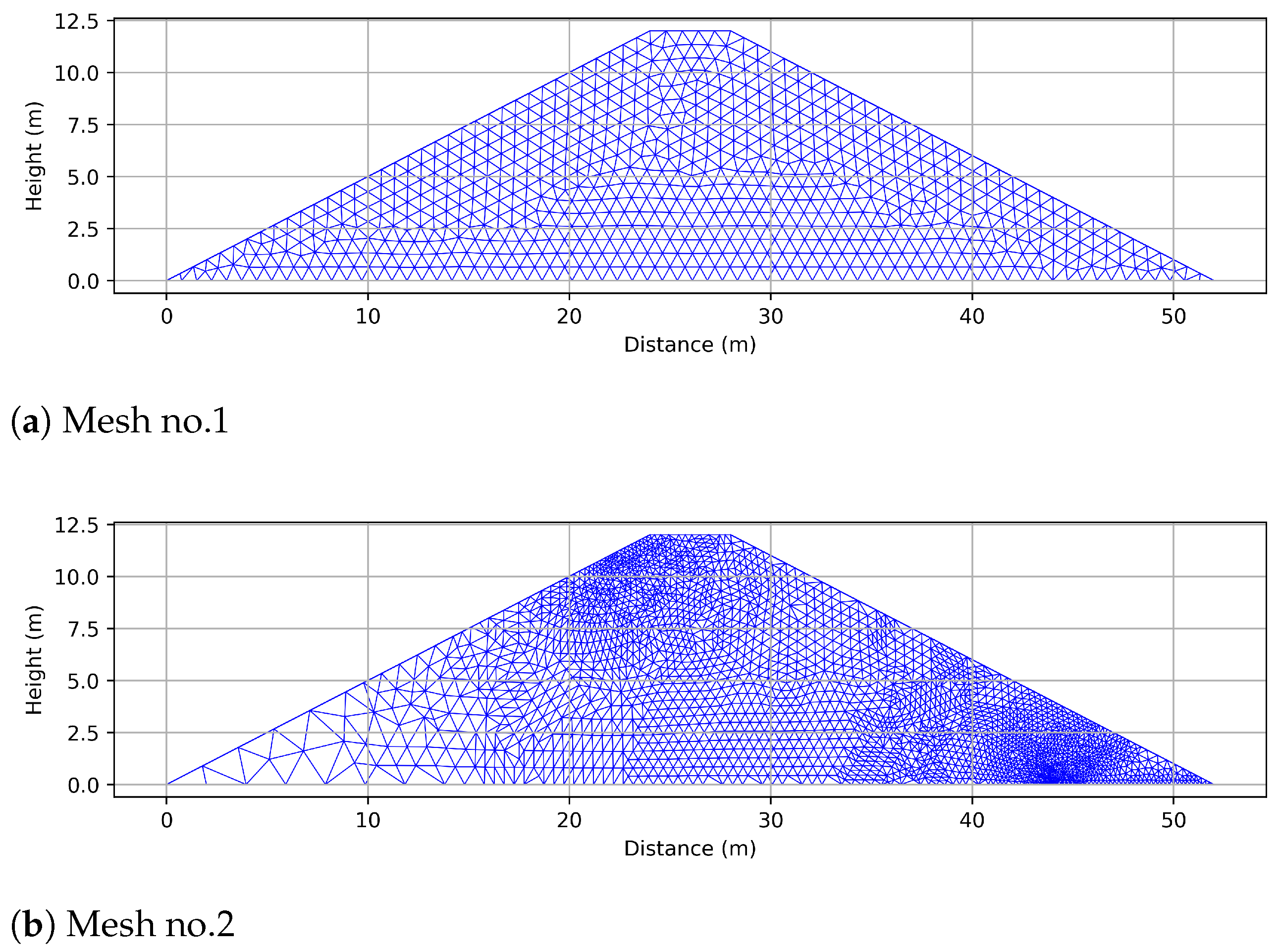
Equation (7) is used for approximating the solution of Equation (4) considering that, at the nodes of a grid, the dependence of $k_x$, $k_y$, $h_w$ and their partial derivatives on the nodes and their corresponding neighbors, which yields a nonlinear discrete system of the form

$$H({\widehat{h}}_w){\widehat{h}}_w+f=0$$

(10)

where $H({\widehat{h}}_w)$ is the assembled matrix of coefficients ${\mathsf{\Gamma }}_0, {\mathsf{\Gamma }}_1,\dots ,{\mathsf{\Gamma }}_k$ obtained at each inner grid node from the solution of Equation (7), ${\widehat{h}}_w$ is the vector of unknown hydraulic head values and f is the vector of boundary values assembled with the known Dirichlet boundary conditions. The matrix H depends on the hydraulic conductivity, which is a function of the unknown variable $h_w$ (through Equations (2) and (3)); thus, the problem becomes nonlinear and an iterative scheme solution must be applied.

Regarding the discrete assembled systems obtained using the proposed discretization, since H shares matrix structures that are common to other numerical methods, namely, finite elements, finite volumes, the finite pointset method, and the radial basis function method, and the solution of such nonlinear systems and their linearizations has been thouroughly studied [7], the focus on the papers remains on the new discretization. Thus, the solution of Equation (10) can be approximated from the following equation:

$${\widehat{h}}_w^{n+1}=-{[H({\widehat{h}}_w^n)]}^{-1}f;$$

(11)

the residual of the equation,

$$\psi ({\widehat{h}}_w^n)=H({\widehat{h}}_w^n){\widehat{h}}_w+f,$$

(12)

is used to correct iteratively the initial assumed value of ${\widehat{h}}_w^n$ as

$${\widehat{h}}_w^{n+1}={\widehat{h}}_w^n+{\alpha }_{k_n}\mathsf{\Delta }{\widehat{h}}_w^n$$

(13)

where

$$\mathsf{\Delta }{\widehat{h}}_w^n=-{[J({\widehat{h}}_w^n)]}^{-1}\psi ({\widehat{h}}_w^n),$$

(14)

${\alpha }_{k_n}$ is the adaptive Armijo’s step length and J is the Jacobian is defined as

$$J({\widehat{h}}_w^n)=H({\widehat{h}}_w^n)+H^{\prime }({\widehat{h}}_w^n).$$

The last term in the Jacobian corresponds to nonsymmetric terms; if it is neglected, the conventional iterative method is obtained. The solution will be reached until the value of $\psi (h_w^n)$ is less than the given tolerance [40].

The adaptive step length ${\alpha }_{k_n}$ was initially set to $0.7$. Whether a sufficient decrease in the residual is not obtained, the step $\mathsf{\Delta }{\widehat{h}}_w^n$ is multiplied by ${\alpha }_{k_n}$.

This Modified Newton–Raphson Method (MNR) was used in the numerical tests of the next section.

2.3. Case of Study

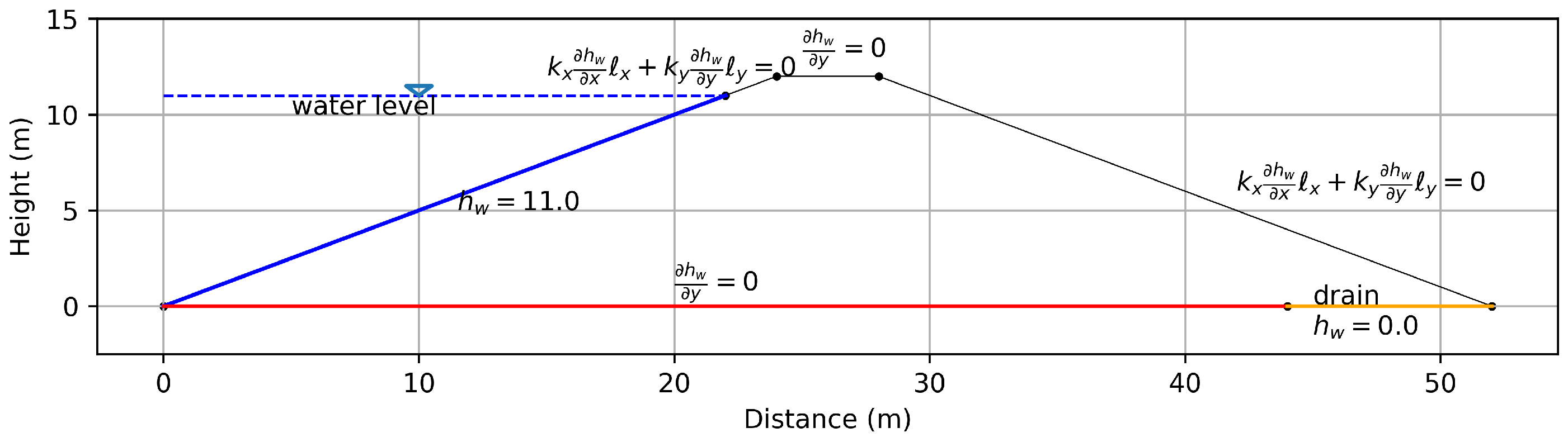
2.3.1. Problem Domain and Boundary Conditions

The domain for the case study is a typical cross-section of a dam of 12 m height; it is shown in Figure 1 along with its boundary conditions. The dam is built of only one kind of soil; the water level is located at 11 m on the upstream side ($h_w=11$). The dam bed is considered impervious except for a drain of 8 m of length placed on the downstream side, where the pore water pressure is set as equal to zero. The downstream boundary condition is also set to zero, with the intensity direction of the normal flux defined by the direction cosines ${\ell }_x$, ${\ell }_y$. The same case is presented in the upper part of the upstream boundary above the water level and at the top of the dam. It must be noted that in the case where the water level exceeds the downstream boundary height, the water pressure equals the atmospheric pressure, and then the boundary conditions must be corrected accordingly.

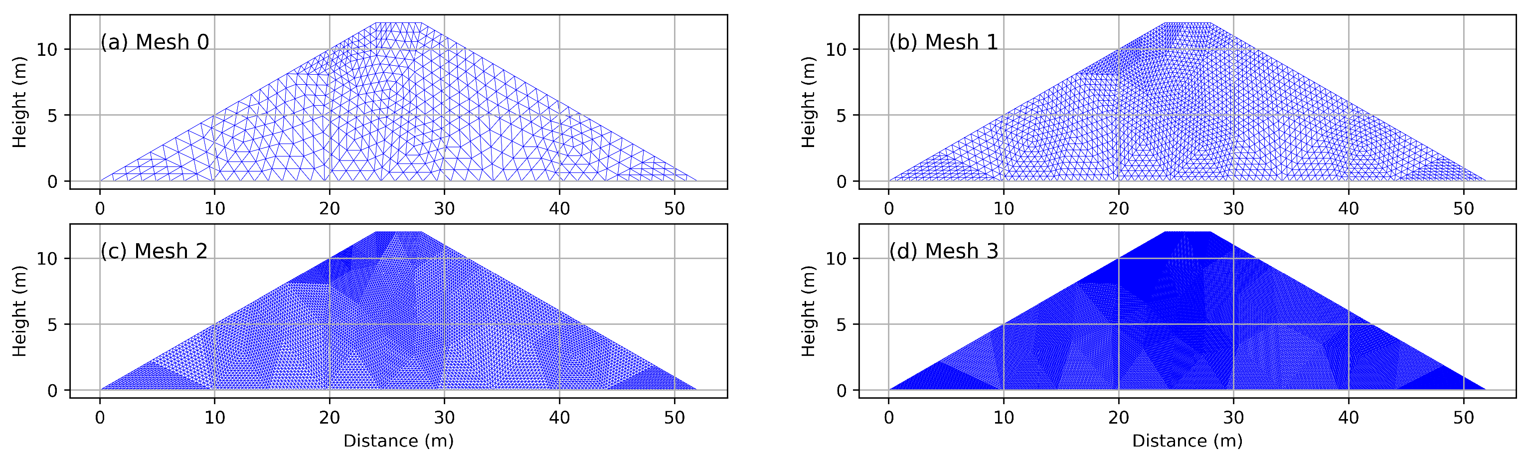
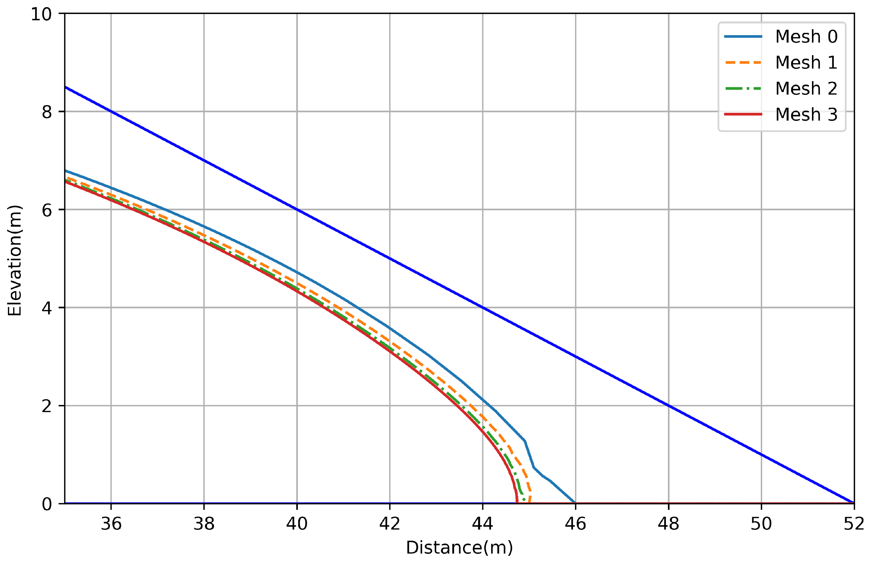
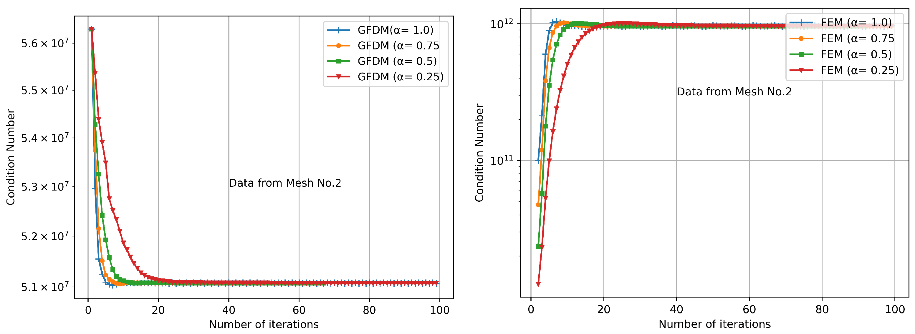
2.3.2. Grid Independence

In order to assess the grid independence of the generalized finite difference discretization as defined by Equation (7), a sequence of four grids for the problem domain was generated. The first one is a coarse mesh with 992 triangles; it was generated using Delaunay triangulation for a set of 553 inner grids nodes obtained from a given initial node distribution. No smoothing process was applied. The next three grids were obtained by a process of refining, on which a splitting procedure was selected; in other words, each triangle was subdivided into four triangles by splitting each triangle side by his midpoint [41].

Following this procedure, grids with 3968, 15,872, and 63,488 triangles were generated (see Figure 2). Using this grids, Equation (10) was solved using the parameters described in Section 2.3.3. The phreatic line for the finest mesh (d) is shown in Figure 3. A more detailed view of the phreatic lines is displayed in Figure 4. The fast approximation of the consecutive phreatic lines to the one corresponding to the finest mesh can be seen, even though the meshes were not smoothed or preprocessed.

In

Table 1. RMSE errors from the phreatic curves calculated in the meshes.

Mesh	A	B
Mesh 0	0.03572126729978147	0.09399951295707337
Mesh 1	0.00629495397038204	0.01468723574184271
Mesh 2	0.00213435762711308	0.00213435762711308

, a summary of the root mean square errors (RMSE) between the different phreatic levels obtained is shown. The values in the column labeled as A correspond to RMSE errors between the phreatic curve for a mesh and the phreatic level for its refinement. In the third column, labeled as B, the phreatic level obtained for Mesh 3 (see Figure 2) was taken as the reference to calculate the RMSE errors. The values in the table are consistent with the fact that the phreatic levels in the coarser grids tend to the last one, thus assessing grid independence for the proposed discretization.

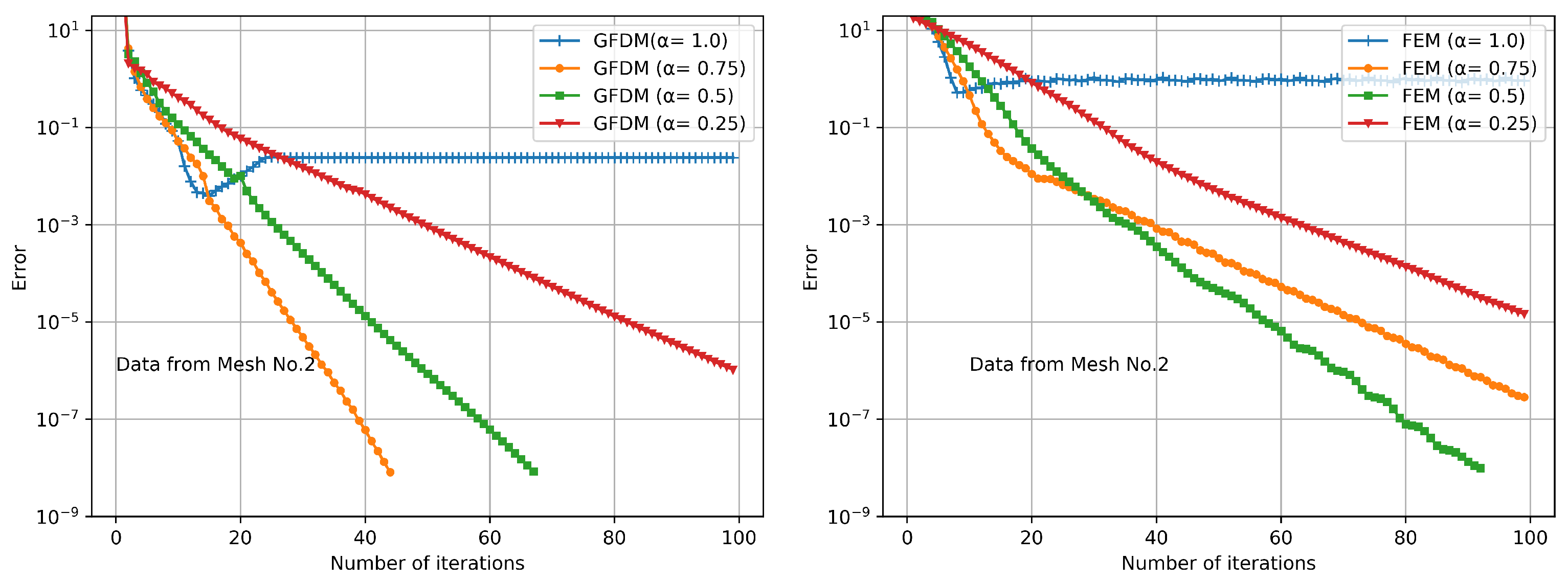
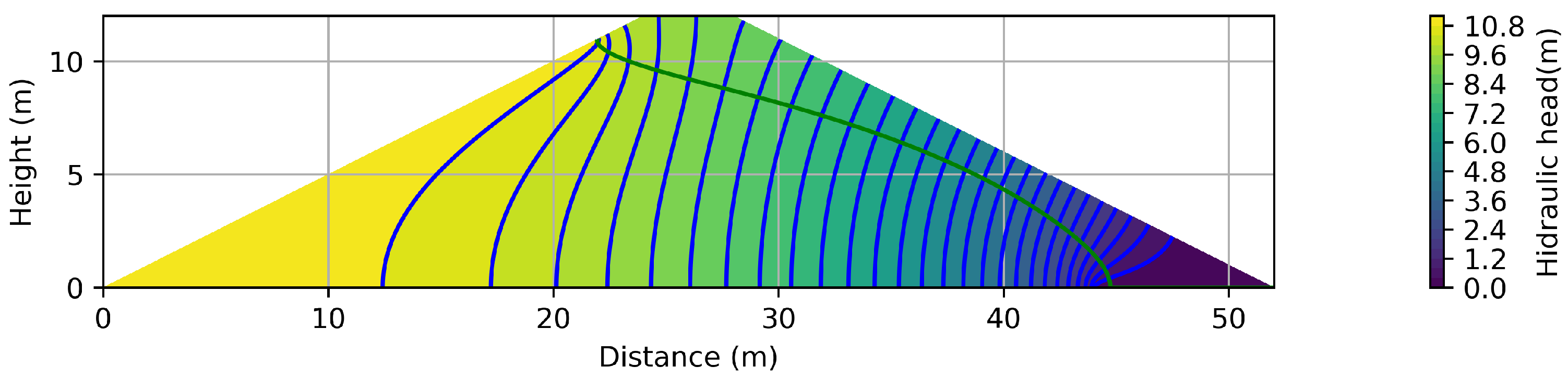
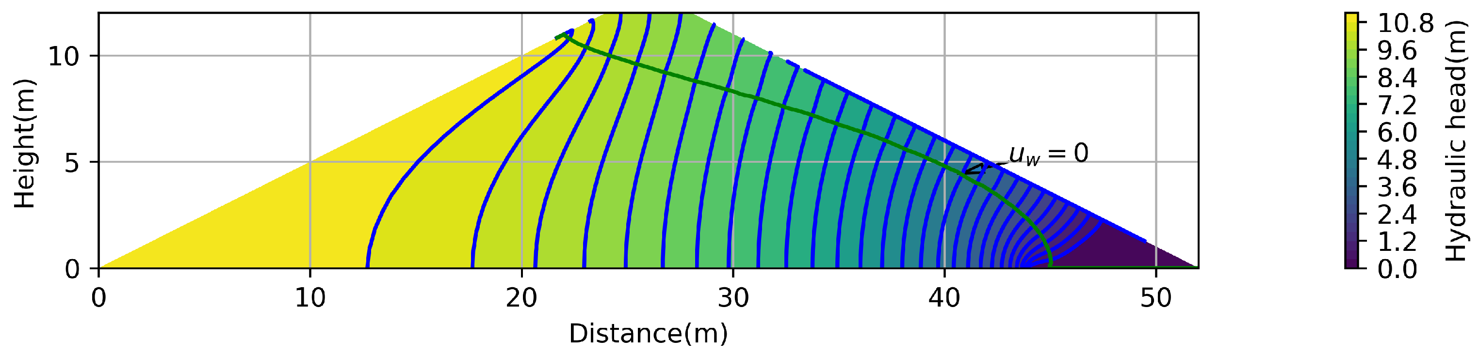
2.3.3. Stationary Flow in a Dam

Regarding the problem of interest, the modeling stationary flow in a dam was solved with two numerical methods: the generalized finite differences method described in the previous section and the finite element method using linear elements as a reference. Both of them were codified in Julia 1.5. Having the shape of the phreatic levels obtained in the previous subsection, two new different meshes were used in the numerical experiments: a rather coarse one (Figure 5a) and another with refinement in the zones where abrupt changes in $\partial h_w/\partial x$ (Figure 5b) are expected. The first mesh has 778 nodes and 4221 triangular elements with an approximate side length of 0.75 m. The refined mesh has 2559 nodes and 14,661 elements and was obtained from the coarse one by refining around the boundary sides where Dirichlet and Neumann boundary conditions meet.

The soil parameters used in the tests are shown in

Table 2. Soil parameters used in the simulation.

Parameter	Value
$\theta r$	0.05
$\theta s$	0.5
$\alpha$ (1/kPa)	0.86
n	1.57
ks (m/s)	$1.0\times {10}^{-6}$

. The finite element method solution in the refined mesh is shown in Figure 6, where the line at $u_w=0$ is the phreatic line. For the next analysis, it will be taken as a reference for the comparison of the different solutions presented.

As mentioned, the Newton–Rapson method was used to solve the discretized nonlinear Richards equations. To evaluate the performance of the GFDM compared to that of the FEM method, the number of iterations required to achieve convergence in the solution in both methods with the two meshes is presented. The algorithm uses two-stop criteria: the relative tolerance error (set to $1.0\times {10}^{-8}$) as the convergence criterion and a maximum number of iterations (100) to avoid endless or slow loops; the first occurrence breaks the cycle.

The root mean square error (RMSE) along the reference phreatic line was calculated with the Equation (15),

$${ϵ}_r=\sqrt{\frac{\mathsf{\Sigma }{(h_{fd}-h_{fe})}^2}{N}},$$

(15)

where:

$h_{fd}$ is the finite differences approximation to the hydraulic head;

$h_{fe}$ is the finite element approximation to the hydraulic head;

N is the number of measurements along the reference line.

3. Results and Discussion

A zoomed in view of the solution near the drain zone can be seen in Figure 7; the high slope can be easily noticed. In a two-dimensional view, some additional remarkable details can be noted. In Figure 8a, the phreatic line obtained with both methods in the refined mesh is presented. The value of the area enclosed by the solutions is equal to 2.2396 m² in the coarse mesh and the value of the RMSE is equal to 0.1152 m. However, if one looks at Figure 8a in detail, near the base there is a separation of the two calculated lines. The one in blue (FEM method) has a slight shift to the right, an effect that occurs due to the mesh, whereas the red line (GFDM method) is completely vertical. This suggests that the GFDM solution is smoother than the FEM solution near the base. To highlight the effect of the mesh mentioned above, in Figure 8b, the solution with the coarse mesh is shown. The separation of the two lines increases and this causes the RMSE error and enclosed areas to increment to 0.1969 and 2.2414 m², respectively, due to abrupt movements of the blue line (FEM results) caused by the singularity at the boundary. As a reference, the maximum distance between the two lines is printed in the figures (max error), and it can be noted that, for coarse mesh, its value is 0.7268 m, and for the refined one, it is equal to 0.2772 m; these numbers confirm the observation mentioned above.

The analysis of the performance of the Newtonian iteration (13) provides some extra insight into the solution process. The semilogarithmic Figure 9 and Figure 10 present the convergence history for solving the problem on both grids; Figure 9 shows results on the coarse grid. Clearly, on the coarse grid, even when in both cases convergence is achieved, the FEM iteration shows a better performance. On the other hand, on the refined mesh, adapting the step size length under the Armijo rule was necessary to achieve convergence, the GFDM being notably faster in the latter case.

Additionally, Figure 11 and Figure 12 show the evolution of the Jacobian condition number on the iterations. In both cases, the condition numbers are relatively large, although the Jacobian on the FEM iteration is in a worse condition than in the case of the GFDM iteration even when the same Newtonian procedure is applied. Nevertheless, when the Armijo rule is applied, convergence was obtained in all the tests.

In

Table 3. Estimated order of convergence for each problem.

Method	Mesh	$\mathit{\alpha }$	LS Slope	Order
GFDM	1	0.25	−0.0211	0.9843
GFDM	1	0.50	−0.0341	0.9947
GFDM	1	0.75	−0.0486	0.9974
GFDM	1	1.00	−0.0642	0.9989
FEM	1	0.25	−0.1017	1.0203
FEM	1	0.50	−0.2147	1.0041
FEM	1	0.75	−0.2172	−1.0301
FEM	1	1.00	−0.1505	0.1884
GFDM	2	0.25	−0.1374	0.9978
GFDM	2	0.50	−0.2772	0.9952
GFDM	2	0.75	−0.4542	2.6186
GFDM	2	1.00	0.0000	−1.3084
FEM	2	0.25	−0.1180	0.9987
FEM	2	0.50	−0.2076	2.2392
FEM	2	0.75	−0.1362	−2.6338
FEM	2	1.00	−0.0001	−3.2192

, a summary of the convergence history for each test is shown. According to the graphs, although in most of the tests there is convergence, the error sequences behave quite differently. In the coarse grid, numbered as 1, the FEM iteration is faster, but the estimated convergence order in the table in both cases is essentially the same. It must be pointed out that to produce a fair comparison, the reported value of the estimated empirical order corresponds to the average of the last 40 iterations. Thus, the oscillations shown in the FEM iterations, which do not avoid convergence, are smoothed for the analysis. However, despite the oscillations, there is a clear graphical trend that shows a better performance. The value of the Least Squares Slope (LS Slope), taken in the same last 40 iterations, corroborates this fact.

On the other hand, when the grid is refined, convergence cannot be achieved without the Armijo adapting step size length strategy. It can be seen that, in both methods, convergence is accelerated, with the value $\alpha =0.75$ being the one the produces the best results. The convergence order is notably larger, but now the LS Slopes show that the GFDM iterations produce a faster iteration.

4. Conclusions

As the main conclusion, it is possible to state that the GFDM is a useful numerical technique to solve several differential equations of interest—in the present case, the steady Richards’ equation was used, which is a nonlinear expression. As a numerical method, GFDM keeps most of the simplicity of the standard formulation on rectangular grids, but can also be applied to nonstructured meshes. In the proposed tests, carried out under the same conditions and taking advantage of a suitable Newtonian iteration and an adaptive step length strategy, the GFDM was capable of achieving convergence faster than FEM in the refined mesh. Additionally, the calculated GFD solution shows a much smoother convergence history than the FEM solution, even in the presence of a singularity at the boundary, a characteristic that may be useful to improve the iterative solution of the discrete assembled systems on infiltration modeling and similar problems.

Considering the diverse applications addressed in the introduction, as well as the results shown in this paper, GFDM stands as a reliable alternative numerical method to solve some differential equations used in applied engineering. Nevertheless, it is convenient to test this numerical technique with other problems to gain a deeper understanding of its capabilities.

References

1. Kaufmann, J.E. Catastrophic Sinkhole Collapse in Missouri. 2007. Available online: https://pubs.usgs.gov/fs/2007/3060/ (accessed on 4 May 2021).
2. Voight, B.; Faust, C. Frictional heat and strength loss in some rapid landslides: Error correction and affirmation of mechanism for the Vaiont landslide. Geotechnique 1992, 42, 641–643. [Google Scholar] [CrossRef]
3. Kilburn, C.R.; Petley, D.N. Forecasting giant, catastrophic slope collapse: Lessons from Vajont, Northern Italy. Geomorphology 2003, 54, 21–32. [Google Scholar] [CrossRef]
4. Richards, L.A. Capillary conduction of liquids through porous mediums. J. Appl. Phys. 1931, 1, 318–333. [Google Scholar] [CrossRef]
5. Zha, Y.; Yang, J.; Zeng, J.; Tso, C.H.M.; Zeng, W.; Shi, L. Review of numerical solution of Richardson—Richards equation for variably saturated flow in soils. WIREs Water 2019, 6, 1–23. [Google Scholar] [CrossRef]
6. Farthing, M.W.; Ogden, F.L. Numerical Solution of Richards’ Equation: A Review of Advances and Challenges. Oil Sci. Soc. Am. J. 2018, 81, 1257–1269. [Google Scholar] [CrossRef] [Green Version]
7. List, F.; Radu, F. A study on iterative methods for solving Richards’ equation. Comput. Geosci. 2016, 20, 341–353. [Google Scholar] [CrossRef] [Green Version]
8. Celia, M.; Bouloutas, E.T.; Zarba, R.L. A general mass-conservative numerical solution for the unsaturated flow equation. Water Resour. Res. 1990, 26, 1483–1496. [Google Scholar] [CrossRef]
9. Howington, S.E.; Berger, R.C.; Hallberg, J.P.; Peters, J.F.; Stagg, A.K.; Jenkins, E.W.; Kelley, C.T. A Model to Simulate the Interaction between Groundwater and Surface Water; Technical Report; US Army Engineering Research and Development Center: Vicksburg, MS, USA, 1999. [Google Scholar]
10. Simunek, J.; van Genuchten, M.; Sejna, M. Development and applications of the HYDRUS and STANMOD software packages and related codes. Vadose Zone J. 2008, 7, 587–600. [Google Scholar] [CrossRef] [Green Version]
11. Trefry, M.G.; Muffels, C. Feflow: A finite-element ground water flow and transport modeling tool. Ground Water 2007, 45, 525–528. [Google Scholar] [CrossRef]
12. Camporese, M.; Paniconi, C.; Putti, M.; Orlandini, S. Surface-subsurface flow modeling with path-based runoff routing, boundary condition-based coupling, and assimilation of multisource observation data. Water Resour. Res. 2010, 46, 1–22. [Google Scholar] [CrossRef] [Green Version]
13. Yeh, G.T.; Shih, D.S.; Cheng, J.R.C. An integrated media, integrated processes watershed model. Comput. Fluids 2011, 45, 2–13. [Google Scholar] [CrossRef]
14. Solin, P.; Kuraz, M. Solving the nonstationary Richards equation with adaptive hp-FEM. Adv. Water Resour. 2011, 34, 1062–1081. [Google Scholar] [CrossRef]
15. Ngo-Cong, D.; Mai-Duy, N.; Antille, D.L.; van Genuchten, M.T. A control volume scheme using compact integrated radial basis function stencils for solving the Richards equation. J. Hydrol. 2020, 580, 1–10. [Google Scholar] [CrossRef]
16. Eymard, R.; Gutnic, M.; Hilhorst, D. The finite volume method for Richards equation. Comput. Geosci. 1999, 3, 259–294. [Google Scholar] [CrossRef]
17. Manzini, G.; Ferraris, S. Mass-conservative finite volume methods on 2-D unstructured grids for the Richards’ equation. Adv. Water Resour. 2004, 27, 1199–1215. [Google Scholar] [CrossRef]
18. Caviedes-Voullième, D.; García-Navarro, P.; Murillo, J. Verification, conservation, stability and efficiency of a finite volume method for the 1D Richards equation. J. Hydrol. 2013, 480, 69–84. [Google Scholar] [CrossRef]
19. Casulli, V.; Zanolli, P. A nested Newton-type algorithm for finite volume methods solving Richards’ equation in mixed form. SIAM J. Sci. Comput. 2010, 32, 2255–2273. [Google Scholar] [CrossRef]
20. Aravena, J.E.; Dussaillant, A. Storm-water infiltration and focused recharge modeling with finite-volume two-dimensional Richards equation: Application to an experimental rain garden. J. Hydraul. Eng. 2009, 135, 1072–1080. [Google Scholar] [CrossRef] [Green Version]
21. Esmaeilzadeh, M.; Barron, R.; Balachandar, R. Numerical Solution of Partial Differential Equations in Arbitrary Shaped Domains Using Cartesian Cut-Stencil Finite Difference Method. Part I: Concepts and Fundamentals. Numer. Math. Theor. Meth. Appl. 2020, 13, 881–907. [Google Scholar] [CrossRef]
22. Fayer, M.H.; Jones, T.L. UNSAT-H Version 2. 0: Unsaturated Soil Water and Heat Flow Model (No. PNL-6779); Technical Report; Pacific Northwest National Laboratory: Richland, WA, USA, 1990. [Google Scholar]
23. Flerchinger, G.N. The Simultaneous Heat and Water (SHAW) Model: Technical Documentation; Technical Report; USDA Agricultural Research Service: Boise, ID, USA, 2000. [Google Scholar]
24. van Dam, J.C.; Feddes, R.A. Numerical simulation of infiltration, evaporation, and shallow groundwater levels with the Richards’ equation. J. Hydrol. 2000, 233, 72–85. [Google Scholar] [CrossRef]
25. Jansson, P.E.; Karlberg, L. Coupled Heat and Mass Transfer Model for Soil-Plant-Atmosphere Systems; Technical Report; Royal Institute of Technology: Stockholm, Sweden, 2010. [Google Scholar]
26. Hsieh, P.A.; Wingle, W.; Healy, R.W. VS2DI—A Graphical Software Package for Simulating Fluid Flow and Solute or Energy Transport in Variably Saturated Porous Media; Technical Report; U.S. Geological Survey: Lakewood, CO, USA, 2000.
27. Domínguez-Mota, F.J.; Mendoza-Armenta, S.; Tinoco-Guerrero, G.; Tinoco-Ruiz, J.G. Finite difference schemes satisfying an optimality condition for the unsteady heat equation. Math. Comput. Simul. 2014, 106, 76–83. [Google Scholar] [CrossRef]
28. Chávez-Negrete, C.; Domínguez-Mota, F.J.; Santana-Quinteros, D. Numerical solution of Richards’ equation of water flow by generalized finite differences. Comput. Geotech. 2018, 101, 168–175. [Google Scholar] [CrossRef]
29. Jensen, P. Finite difference techniques for variable grids. Comput. Struct. 1972, 2, 17–29. [Google Scholar] [CrossRef]
30. Liszka, T.; Orkisz, J. The finite difference method at arbitrary irregular grids and its application in applied mechanics. Comput. Struct. 1980, II, 83–95. [Google Scholar] [CrossRef]
31. Benito, J.J.; Ureña, F.; Gavete, L. Influence of several factors in the generalized finite difference method. Appl. Math. Model. 2001, 25, 1039–1053. [Google Scholar] [CrossRef]
32. Ureña-Prieto, F.; Muñoz, J.J.B.; Gavete-Corvinos, L.A.; Alonso, B. Application of the Generalized Finite Difference Method to Solve the Advection-diffusion Equation. Comput. Appl. Math. 2011, 235, 1849–1855. [Google Scholar] [CrossRef] [Green Version]
33. Milewski, S. Meshless Finite Difference Method with Higher Order Approximation—Applications in Mechanics. Arch. Comput. Methods Eng. 2012, 19, 1–49. [Google Scholar] [CrossRef]
34. Li, T.S.; Wong, S.M. Solving the singular Motz problem using Radial Basis functions. In Proceedings of the 9th International Conference on Computational Methods (ICCM2018), Rome, Italy, 6–10 August 2018. [Google Scholar]
35. Fredlund, D.G.; Rahardjo, H.; Fredlund, M.D. Unsaturated Soil Mechanics in Engineering Practice; John Wiley & Sons: Hoboken, NJ, USA, 2012. [Google Scholar]
36. Mualem, Y. A new model for predicting the hydraulic conductivity of unsaturated porous media. Water Resour. Res. 1976, 12, 513–522. [Google Scholar] [CrossRef] [Green Version]
37. Genuchten, M.T.V. A closed-form equation for predicting the hydraulic conductivity of unsaturated soils. Soil Sci. Soc. Am. J. 1980, 44, 892–898. [Google Scholar] [CrossRef] [Green Version]
38. Jefferies, A.; Kuhnert, J.; Aschenbrenner, L.; Giffhorn, U. Finite pointset method for the simulation of a vehicle travelling through a body of water. In Meshfree Methods for Partial Differential Equations VII; Springer: Berlin/Heidelberg, Germany, 2015; pp. 205–221. [Google Scholar]
39. Kellogg, R.B. Difference equations on a mesh arising from a general triangulation. Math. Comput. 1964, 18, 203–210. [Google Scholar] [CrossRef]
40. Lyness, J.F.; Owen, D.R.J.; Zienkiewicz, O.C. The finite element analysis of engineering systems governed by a non-linear quasi-harmonic equation. Comput. Struct. 1975, 5, 65–79. [Google Scholar] [CrossRef]
41. George, P. Automatic Mesh Generation: Application to Finite Element Method; Wiley Publishers: Hoboken, NJ, USA, 1991. [Google Scholar]
Short Biography of Author
Mathematics 09 01604 i001Carlos Chávez-Negrete is a professor of in the Civil Engineering School of the Universidad Michoacana de San Nicolás de Hidalgo (UMSNH) in Morelia, Mexico. He holds a Ph.D. in Geotechnical Engineering from Universitat Politècnica de Catalunya, in Spain. His research interest includes laboratory characterization of soils and rocks, slope stability analysis, pavement analysis, and design, the development of numerical methods for geotechnical engineering, and unsaturated soil mechanics.
Mathematics 09 01604 i002Francisco Domínguez-Mota completed a B.Sc. in Physics and Mathematics at the Universidad Michoacana in México. He obtained a Master degree in Applied Mathematics from the Center of Research in Mathematics in Guanajuato, Mexico, and a Ph.D in Mathematics at the Universidad Nacional Autónoma de México. He is a member of the National System of Researchers (SNI) in México, and is a researcher in Applied Mathematics at the Universidad Michoacana. His areas of research include numerical solution of differential equations and applications in engineering, numerical generation of structured grids and applications of optimization in large scale problems.
Mathematics 09 01604 i003Daniel Santana-Quinteros is a M.Sc. student at the Centro de ciencias matemáticas UNAM campus Morelia. He completed a B.Sc. in Physics and Mathematic at the Universidad Michoacana in México. He has been a math teacher since 2018. His areas of research include numerical solution of differential equations, flow in porous media, biomathematics and systems biology.
Figure 1. Scheme of the flow dam problem.
Mathematics 09 01604 g001
Figure 2. Grids with (a) 992 triangles, (b) 3968 triangles, (c) 15,872 triangles, (d) 63,488 triangles.
Mathematics 09 01604 g002
Figure 3. The phreatic level calculated in the finest mesh (d) shown in Figure 2.
Mathematics 09 01604 g003
Figure 4. Calculated phreatic levels using the grids (a–d) shown in Figure 2.
Mathematics 09 01604 g004
Figure 5. Meshes used in the numerical tests.
Mathematics 09 01604 g005
Figure 6. FEM solution in the refined mesh.
Mathematics 09 01604 g006
Figure 7. Zoomed in view of the solution near the drain at the lower right corner of the cross-section. The high gradient zone can be easily noticed.
Mathematics 09 01604 g007
Figure 8. Comparison between the solution of the two methods.
Mathematics 09 01604 g008
Figure 9. Convergence history on mesh no. 1 (coarse mesh).
Mathematics 09 01604 g009
Figure 10. Convergence history on mesh no. 2 (refined mesh).
Mathematics 09 01604 g010
Figure 11. Jacobian condition number history on mesh no. 1 (coarse mesh).
Mathematics 09 01604 g011
Figure 12. Jacobian condition number history on mesh no. 2 (refined mesh).
Mathematics 09 01604 g012