Jump-Diffusion Models for Valuing the Future: Discounting under Extreme Situations

Abstract

We develop the process of discounting when underlying rates follow a jump-diffusion process, that is, when, in addition to diffusive behavior, rates suffer a series of finite discontinuities located at random Poissonian times. Jump amplitudes are also random and governed by an arbitrary density. Such a model may describe the economic evolution, specially when extreme situations occur (pandemics, global wars, etc.). When, between jumps, the dynamical evolution is governed by an Ornstein–Uhlenbeck diffusion process, we obtain exact and explicit expressions for the discount function and the long-run discount rate and show that the presence of discontinuities may drastically reduce the discount rate, a fact that has significant consequences for environmental planning. We also discuss as a specific example the case when rates are described by the continuous time random walk.

1. Introduction

The importance of discounting, particularly in the long run, does not exclusively refer to finance, but to many aspects of global economy. This is the case of long-term environmental planning, which is certainly acute in climate action. In essence, an environmental disaster that could cost X to repair at a future time t is worth $exp(-rt)X$ today, where r is the interest rate assuming that is continuously compounded. This simple analysis assumes that interest rates remain constant between today and the distant future t, which may be decades ahead. The rate r thus becomes a key magnitude to decide whether it is more beneficial to take action today with a significant investment or whether the discount gives negligible value to today’s investment.

No wonder that the estimation of the discount rate has enormous consequences and has been the object of intense work and controversy for a long time. While, for instance, the reputed and highly influential British economist Nicholas Stern [1] had been using a discounting rate of $1.4\%$, William Nordhaus [2] did propose a discount rate of $4\%$ and even a higher rate ($6\%$) [3]. The two estimates stand for very different perspectives on how to face climate change and other catastrophic events. Stern’s rate entails for an immediate spending, and Nordhaus’s figures say that action could be less urgent and not that strong. The choice of discount rate lays at the center of the debate on the urgency of climate change mitigation.

When we refer to climate, discount rates choice is based on ethical grounds [4,5] and on future economic growth assumptions. Economic arguments involve the maximization of utility functions [6]. Discounting not only includes economic growth; it also includes behavioral aspects such as impatience or the possibility of having a declining marginal utility. All of these aspects are covered in the Ramsey formula [7], which constitutes the basis of the more traditional approach to discounting [8]. It is, however, not realistic to represent discounting by deterministic functions of time. To consider decreasing exponentials with fixed rates is then too simplistic and it is necessary to consider an average overall interest rate path. In global warming, this issue becomes particularly sensitive as one must consider costs and benefits for long time horizons. Quantitative finance has indeed provided a robust framework (e.g., the so called Heath–Jarrow–Morton framework) [9], while several works have long recognized that interest rates must be modeled as random processes [10,11,12,13,14].

An economist working with statistics might decide to compute the discount rate as the average over empirical interest rates during the last 200 years (which is 2.7% in stable countries [15,16]), or estimate the average of Wall Street forward looking models with the 30 year bond prices. However, our recent work [17] shows that the rate is considerably below these averages, and this can be attributed to historical fluctuations. As a result, any proper analysis must take into account fluctuations in the real interest rate (obtained by subtracting nominal rates from inflation), which are fundamentally due to fluctuations in economic growth [18,19,20,21,22].

The function $r\left(t\right)$ can, in principle, be described by any random process. Markovian processes are the simplest and most common hypothesis and they consist of continuous sample paths. In other words, real rates $r\left(t\right)$ are modeled as diffusion processes. Throughout this paper, we will assume the so-called “Local Expectation Hypothesis”, in which there is no market price of risk (investors are assumed to be risk neutral) and rates are based on the data generating measure [23,24,25].

We have been analyzing these issues by assuming three of the most popular stochastic models for the dynamics of interest rates [26]: Ornstein–Uhlenbeck [27], Feller [28], and log-normal [29] processes, which are also relevant in the context of statistical physics. However, we are interested in real rates which can be negative even during prolonged periods of time [15,17]: recall, real rates are nominal rates corrected by inflation, that is, $r\left(t\right)=n\left(t\right)-i\left(t\right)$, where $n\left(t\right)$ are nominal rates (usually positive, but not always) and computed from government bonds, and $i\left(t\right)$ is the rate of inflation constructed out of consumer price indexes. The Ornstein–Uhlenbeck (OU) model is the only one that allows for negative rates while still considering simplest (and linear) mean reversion towards a normal interest rate. Moreover, discount asymptotic expression thus has an exponential decay with a long-run rate $r_{\infty }$ that differs from historical average interest rates by being substantially smaller, zero or eventually negative [15,16,17,26,30].

We will go one step further and assume that, in addition to diffusive and continuous behavior, the sample paths of real rates $r\left(t\right)$ also exhibit discontinuities. That is, we will model rates by a jump-diffusion process. During the last fifty years, jump-diffusion models have been extensively used not only in many branches of statistical mechanics and condensed matter physics [31], but also in economics and finance [32,33]. Specially relevant here is the work by Ahn and Thompson [13], which in 1988 already added jumps to a quite general diffusion model to investigate the effect of discontinuities on interest rates and highlighted the effects with the Feller process [28] (also called Cox–Ingersoll–Ross model [23]). Thus, the economic evolution is known to occasionally have sudden bursts that hardly adjust to continuous diffusion-like evolution. The fact that these discontinuities do not occur frequently sustains in a great measure the use of diffusion models for the economic evolution. However, many empirical observations of economic time series tend to show the appearance of many outliers in which changes of great magnitude occur during small intervals of time, in opposition to the basic diffusive hypothesis for which changes during short intervals of time are only by small amounts.

One very recent example is provided by the COVID-19 pandemics, where prices dropped worldwide approximately $40\%$ in less than 3 weeks. Pandemic episodes are rather recurrent, thus during the 20th century, there have been reported several pandemic incidents from the Spanish flu of 1918 to the Hong Kong flu in 1968 or AIDS starting in 1981. Several similar episodes are reported during the 19th century (cholera, etc.). One could approximately quantify the appearance of 3 to 5 of such episodes per century. Other “nightmare scenarios” [34,35] of environmental disasters would include climate change, biotechnology, asteroid impacts, runaway computer systems, and nuclear proliferation, among others (see Refs. [36,37] for a thorough discussion).

The main objectives of this work are to provide a general framework and to elucidate the effect on the long-run discount—and, hence, on how we should value the future—of discontinuities that reflect the existence of high-risk events. For the sake of completeness, we consider not only sudden negative bursts, but also positive bursts as the two show distinctive behaviors.

Section 2 has two parts. Section 2.1 provides the main and broad definitions being used for the analysis, and Section 2.2 presents the specificities of the Ornstein–Uhlenbeck jump-diffusion process to model interest rates. The first paragraphs in Section 3 provide the main result. Section 3.1 presents the asymptotic discount function jointly with the long-run discount rate. Two specific jump distributions are studied in Section 3.2: fixed jump amplitudes and Laplacian jump amplitudes. Before a final discussion and the conclusions, Section 3.3 finally provides the discount within the continuous time formalism, that is: a purely discontinuous process.

2. Materials and Methods

2.1. Main Definitions

Suppose that $r\left(t\right)$ is a random process representing the dynamical evolution of real rates. If we define the cumulative process

$$x\left(t\right)={\int }_{t_0}^{t}r\left(t^{\prime }\right)d{t}^{\prime },$$

(1)

the discount function is then defined as

$$D\left(t\right)=\mathbb{E}\left[e^{-x\left(t\right)}\right],$$

(2)

where the average is taken over all possible realizations of $r\left(t\right)$ and market price of risk is assumed to be zero (see our previous work [16]). “Local Expectation Hypothesis” in which there is no market price of risk (investors are assumed to be risk neutral) is considered [23,24,25].

Closely related to the discount function, $D\left(t\right)$ is the (average) discount rate defined as

$$d\left(t\right)=-\frac{lnD\left(t\right)}{t},$$

(3)

so that the discount function can be written in the standard exponential form $D\left(t\right)=exp(-td(t\left)\right)$. Moreover, in terms of $d\left(t\right)$, we can define the long-run discount rate, $r_{\infty }$, as the asymptotic value of the discount rate $d\left(t\right)\to r_{\infty }$ as $t\to \infty$. That is,

$$r_{\infty }=-\underset{t\to \infty }{lim}\frac{ln\left(D\right(t\left)\right)}{t}.$$

(4)

When introducing specific stochastic models, it then becomes particularly useful to consider the bidimensional process $\left(x\left(t\right),r\left(t\right)\right)$ and denote by $p(x,r,t|x_0,r_0,t_0)$ the probability density function (PDF) of such process (sometimes referred to as the data generating measure). This PDF is defined as

$$p(x,r,t|x_0,r_0,t_0)dxdr=\mathrm{Prob}\left\{x\le x\left(t\right)<x+dx,r\le r\left(t\right)<r+dr|x\left(t_0\right)=x_0,r\left(t_0\right)=r_0\right\},$$

and the discount function defined as the average (2) can therefore be written as

$$D\left(t\right)={\int }_{-\infty }^{\infty }dr{\int }_{-\infty }^{\infty }{e}^{-x}p(x,r,t|x_0,r_0,t_0)dx.$$

(5)

The joint characteristic function of the bidimensional process $\left(x\right(t),r(t\left)\right)$ is defined as the Fourier transform of the joint PDF:

$$\tilde{p}({\omega }_1,{\omega }_2,t|x_0,r_0,t_0)={\int }_{-\infty }^{\infty }{e}^{-i{\omega }_{1}x}dx{\int }_{-\infty }^{\infty }{e}^{-i{\omega }_{2}r}p(x,r,t|x_0,r_0,t_0)dr.$$

(6)

Once we know the joint characteristic function obtaining discount is straightforward. Comparison of Equations (5) and (6) shows that

$$D\left(t\right)=\tilde{p}({\omega }_1=-i,{\omega }_2=0,t|x_0,r_0,t_0),$$

(7)

and obtaining the discount function is equivalent to knowing the joint characteristic function of the bidimensional return process.

2.2. Diffusion Process in the Presence of Random Jumps

The process $r\left(t\right)$ can be any random process, although the simplest and most usual assumption consists in modeling $r\left(t\right)$ as a diffusion process, that is, a Markovian process with continuous sample paths. We here take the further step of assuming that $r\left(t\right)$ is a compound process that combines an ordinary diffusion with random jumps. The diffusion process trajectory thus exhibits discontinuities at random instants of time. Discontinuities will here be assumed to be finite. The resulting bidimensional process $\left(x\right(t),r(t\left)\right)$ is described by the following pair of stochastic differential equations (all stochastic differential equations are interpreted in the sense of Itô):

$$\begin{array}{ccc}\hfill \frac{dx}{dt}& =& r\hfill \\ \hfill \frac{dr}{dt}& =& f\left(r\right)+g\left(r\right)\xi \left(t\right)+n\left(t\right),\hfill \end{array}$$

(8)

where $f\left(r\right)$ and $g\left(r\right)$ are given functions (the drift and noise intensity, respectively), $\xi \left(t\right)$ is a zero-mean Gaussian white noise ($\xi \left(t\right)dt=dW\left(t\right)$ where $W\left(t\right)$ is the standard Wiener process with unit variance), and $n\left(t\right)$ is a white shot noise. The white shot noise can be written as [38,39]

$$n\left(t\right)=\sum _j{\gamma }_j\delta (t-t_j),$$

(9)

where ${\gamma }_j$ and $t_j$ ($j=1,2,3\cdots$) are independent and identically distributed random variables. The random quantities ${\gamma }_i$ characterize the size of jumps and are described by a given PDF, which we denote by $h\left(u\right)$. For simplicity, the size of these discontinuities are taken to be identically distributed and independent of each other as well as independent of the instants of time at which they occur. We further assume that these random times form a Poisson set of events. In such a case, the time interval $\tau$ between two consecutive jumps $\{t_j,t_{j+1}\}$ is governed by the PDF [40]

$$\psi \left(\tau \right)=\lambda e^{-\lambda \tau },$$

(10)

where $\lambda >0$ is the rate of the Poisson process and ${\lambda }^{-1}$ is the average time interval between two consecutive jumps.

To obtain the discount we need to look at the joint PDF $p(x,r,t|x_0,r_0,t_0)$ of the bidimensional process $\left(x\right(t),r(t\left)\right)$. It is, however, convenient to first consider the jump PDF characterizing the discontinuities of the return process. This density is defined as [31]

$$W(x,r|x_0,r_0)=\underset{\Delta t\to 0}{lim}\left[\frac{1}{\Delta t}p(x,r,t_0+\Delta t|x_0,r_0,t_0)\right],$$

A standard reasoning—based on the Chapman–Kolmogorov equation and detailed in Gardiner’s monograph [31] (see also [40]) shows that the PDF of the bidimensional jump-diffusion process defined in (8) obeys the integro-differential equation -4.6cm0cm

$$\begin{array}{ccc}\hfill \frac{\partial p}{\partial t}=& -& r\frac{\partial p}{\partial x}-\frac{\partial }{\partial r}\left[f\left(r\right)p\right]+\frac{1}{2}\frac{{\partial }^2}{\partial r^2}\left[g^2\left(r\right)p\right]\hfill \\ & +& {\int }_{-\infty }^{\infty }dy{\int }_{-\infty }^{\infty }\left[W(x,r|y,\rho )p(y,\rho ,t|x_0,r_0,t_0)-W(y,\rho |x,r)p(x,r,t|x_0,r_0,t_0)\right]d\rho ,\hfill \end{array}$$

(11)

with the initial condition

$$p(x,r,t_0|x_0,r_0,t_0)=\delta (x-x_0)\delta (r-r_0).$$

(12)

The assumptions made above about discontinuities allow us to obtain a a more explicit expression for both the transition density W and the integro-differential Equation (11). Let us recall that the magnitude of the discontinuities, expressed by the random variables ${\gamma }_i$, is independent of the times $t_i$ where jumps occur. We see from the model expressed by Equation (8) that the instantaneous jumps only affect $r\left(t\right)$, but not $x\left(t\right)$. These considerations, along with the Poisson character of jump times, allow us to take as transition density the following expression [40]:

$$W(x,r|x_0,r_0)=\lambda \delta (x-x_0)h(r-r_0).$$

(13)

Substituting this simpler expression for W into Equation (11) and taking into account the homogeneity of both x and t (which amounts to take $x_0=0$ and $t_0=0$) as well as the normalization condition on the PDF $h\left(u\right)$,

$${\int }_{-\infty }^{\infty }h\left(u\right)du=1,$$

we see that the integro-differential equation for $p(x,r,t|r_0)$, Equation (11) reads

$$\begin{array}{ccc}\hfill \frac{\partial p}{\partial t}=-r\frac{\partial p}{\partial x}& -& \frac{\partial }{\partial r}\left[f\left(r\right)p\right]+\frac{1}{2}\frac{{\partial }^2}{\partial r^2}\left[g^2\left(r\right)p\right]\hfill \\ & -& \lambda p(x,r,t|r_0)+\lambda {\int }_{-\infty }^{\infty }h(r-\rho )p(x,\rho ,t|r_0)d\rho ,\hfill \end{array}$$

(14)

and the initial condition is

$$p(x,r,0|r_0)=\delta \left(x\right)\delta (r-r_0).$$

(15)

Equation (14) is the most general formulation of the discount problem of time-homogeneous diffusion with independent and Poissonian random jumps. In order to proceed further we need to further specify a particular diffusion process for the continuous part of the return.

The Ornstein–Uhlenbeck Process and Poissonian Jumps

In the modeling of financial interest rates, the Ornstein–Uhlenbeck (OU) diffusion process was proposed by Oldrich Vasicek during the late nineteen seventies [10]. The model allows for both positive and negative rates and is, therefore, suitable for describing the so-called real interest rates. We have extensively used this process in the study of long-run discounting [15,16,17,26]. For the OU process, the drift is linear and the noise intensity constant:

$$f\left(r\right)=-\alpha (r-m),g\left(r\right)=k.$$

(16)

The parameter m (usually referred to as “normal level”) is the mean value to which the process reverts in the long run, $\alpha >0$ is the strength of the reversion to the mean, and $k>0$ is the amplitude of the fluctuations. In the stationary regime when $t\gg {\alpha }^{-1}$ rates are explicitly given by [26]

$$r\left(t\right)=m+k{\int }_{-\infty }^t{e}^{-\alpha (t-t^{\prime })}\xi \left(t^{\prime }\right)d{t}^{\prime },$$

where $\xi \left(t\right)$ is the Gaussian white noise defined above. We, thus, easily see that the normal level m is the stationary mean value of the return, while the stationary autocorrelation function $C\left(\tau \right)$ is given by [26]

$$C\left(\tau \right)=\left(\frac{k^2}{2\alpha }\right)e^{-\alpha \tau }$$

showing that ${\alpha }^{-1}$ is the autocorrelation time and ${\sigma }^2=k^2/2\alpha$ is the variance. For this continuous model, we have been able to obtain a closed expression for the discount function $D\left(t\right)$, which in the long run, as $t\to \infty$ (cf. Equation (4)), reads [26]

$$D\left(t\right)\simeq e^{-r_{\infty }t},r_{\infty }=m-k^2/2{\alpha }^2.$$

(17)

Let us now assume that the rate process $r\left(t\right)$ is governed by an OU process with random discontinuities described by Poissonian jumps. The integro-differential equation for the joint PDF $p(x,r,t|r_0)$ will be given by (cf. Equations (14) and (16))

$$\begin{array}{ccc}\hfill \frac{\partial p}{\partial t}=& -& r\frac{\partial p}{\partial x}+\alpha \frac{\partial }{\partial r}\left[(r-m)p\right]+\frac{1}{2}{k}^2\frac{{\partial }^{2}p}{\partial r^2}\hfill \\ & -& \lambda p(x,r,t|r_0)+\lambda {\int }_{-\infty }^{\infty }h(r-\rho )p(x,\rho ,t|r_0)d\rho ,\hfill \end{array}$$

(18)

with the initial condition

$$p(x,r,0|r_0)=\delta \left(x\right)\delta (r-r_0).$$

(19)

Fourier transforming Equations (18) and (19) results in a much simpler problem for the characteristic function,

$$\frac{\partial \tilde{p}}{\partial t}=({\omega }_1-\alpha {\omega }_2)\frac{\partial \tilde{p}}{\partial {\omega }_2}-\left[\lambda -\lambda \tilde{h}\left({\omega }_2\right)+i\alpha m{\omega }_2+\frac{k^2}{2}{\omega }_2^2\right]\tilde{p},$$

(20)

where $\tilde{p}=\tilde{p}({\omega }_1,{\omega }_2,t|r_0)$ is the joint Fourier transform defined in Equation (6) and

$$\tilde{h}\left({\omega }_2\right)={\int }_{-\infty }^{\infty }{e}^{-i{\omega }_{2}u}h\left(u\right)du$$

(21)

is the characteristic function of the jump PDF $h\left(u\right)$. The initial condition is now given by

$$\tilde{p}({\omega }_1,{\omega }_2,0|r_0)=e^{-i{\omega }_2{r}_0}.$$

(22)

Equation (20) is a partial differential equation of first order whose solution can be obtained by the method of characteristics [41]. In the Appendix A, we show that the exact solution to the initial-value problem (20) and (22) is given by

$$\tilde{p}({\omega }_1,{\omega }_2,t|r_0)=exp\left\{-\lambda \left[t+\varphi ({\omega }_1,{\omega }_2,t)\right]-A\left(t\right){\omega }_2^2-B({\omega }_1,t){\omega }_2-C({\omega }_1,t)\right\},$$

(23)

where

$$\varphi ({\omega }_1,{\omega }_2,t)={\int }_{{\omega }_2}^{\chi ({\omega }_1,{\omega }_2,t)}\frac{\tilde{h}\left(\theta \right)}{\alpha \theta -{\omega }_1}d\theta ,\chi ({\omega }_1,{\omega }_2,t)=\frac{{\omega }_1}{\alpha }(1-e^{-\alpha t})+{\omega }_2{e}^{-\alpha t},$$

(24)

$$A\left(t\right)=\frac{k^2}{4\alpha }\left(1-e^{-2\alpha t}\right),$$

(25)

$$B({\omega }_1,t)=i{r}_0{e}^{-\alpha t}+im\left(1-e^{-\alpha t}\right)+\frac{k^2{\omega }_1}{2{\alpha }^2}\left(1-2e^{-\alpha t}+e^{-2\alpha t}\right),$$

(26)

and

$$\begin{array}{ccc}\hfill C({\omega }_1,t)& =& i{\omega }_1{r}_0\frac{1}{\alpha }\left(1-e^{-\alpha t}\right)+im{\omega }_1\left[t-\frac{1}{\alpha }\left(1-e^{-\alpha t}\right)\right]\hfill \\ & & +\frac{k^2{\omega }_1^2}{2{\alpha }^3}\left[\alpha t-2\left(1-e^{-\alpha t}\right)+\frac{1}{2}\left(1-e^{-2\alpha t}\right)\right].\hfill \end{array}$$

(27)

Looking at Equation (23), we see that when there are no discontinuities (i.e., $\lambda =0$), the PDF (23) reduces to a Gaussian density as we had obtained in previous works [26]. Denoting this density by $p^{\left(0\right)}$ and setting $\lambda =0$ in Equation (23), we get

$${\tilde{p}}^{\left(0\right)}({\omega }_1,{\omega }_2,t|r_0)=exp\left\{-\left[A\left(t\right){\omega }_2^2+B({\omega }_1,t){\omega }_2+C({\omega }_1,t)\right]\right\}.$$

(28)

We can thus write Equation (23) as

$$\tilde{p}({\omega }_1,{\omega }_2,t|r_0)={\tilde{p}}^{\left(0\right)}({\omega }_1,{\omega }_2,t|r_0)exp\left\{-\lambda \left[t+\varphi ({\omega }_1,{\omega }_2,t)\right]\right\}.$$

(29)

Let us finally recall that knowing the joint PDF of the two-dimensional process $\left(x\right(t),r(t\left)\right)$, the distribution of the return $r\left(t\right)$ is given by the marginal density,

$$p(r,t|r_0)={\int }_{-\infty }^{\infty }p(x,r,t|r_0)dx,$$

and the characteristic function of return, $\tilde{p}({\omega }_2,t|r_0)$, is simply obtained by setting ${\omega }_1=0$ in the joint characteristic function. From Equations (23)–(27), we get

$$\begin{array}{c}\hfill \tilde{p}({\omega }_2,t|r_0)=exp\left\{-\frac{k^2}{4\alpha }\left(1-e^{-2\alpha t}\right){\omega }_2^2-i\left[r_0{e}^{-\alpha t}+m\left(1-e^{-\alpha t}\right)\right]{\omega }_2\right.\\ \hfill \left.-\lambda \left[t+\frac{1}{\alpha }{\int }_{{\omega }_2}^{{\omega }_2{e}^{-\alpha t}}\frac{\tilde{h}\left(\theta \right)}{\theta }d\theta \right]\right\}.\end{array}$$

(30)

In terms of the characteristic function $\tilde{p}({\omega }_2,t|r_0)$, the moments of the return, $\langle r^n\left(t\right)\rangle$, are given by the derivatives $i^n{\tilde{p}}^{\left(n\right)}({\omega }_2=0,t|r_0)$$(n=1,2,\cdots )$. Thus, for example, the variance of the return, that is the volatility, is given by

$${\sigma }^2\left(t\right)=\frac{1}{2\alpha }\left(k^2+\lambda \mu \right)\left(1-e^{-2\alpha t}\right),$$

(31)

where $\mu$ is the second moment of the jump density, $\mu =-{\tilde{h}}^{\prime \prime }\left(0\right)$. In the long-range ($t\to \infty$) the volatility reaches the stationary value

$${\sigma }_{\mathrm{stat}}^2=\frac{1}{2\alpha }\left(k^2+\lambda \mu \right).$$

(32)

3. Results

We know that in terms of the characteristic function of the bidimensional process $\left(x\right(t),r(t\left)\right)$ the discount function $D\left(t\right)$ is given by (cf. Equation (7))

$$D\left(t\right)=\tilde{p}({\omega }_1=-i,{\omega }_2=0,t|r_0).$$

Then from Equation (29) we see that

$$D\left(t\right)=D^{\left(0\right)}\left(t\right)e^{-\lambda [t+\varphi (t\left)\right]},$$

(33)

where $D^{\left(0\right)}\left(t\right)$ is the discount function for the continuous process in the absence of jumps and $\varphi \left(t\right)\equiv \varphi (-i,t)$. The explicit form of these quantities is, respectively, given by (cf. Equations (27) and (24))

$$\begin{array}{c}\hfill D^{\left(0\right)}\left(t\right)=exp\{-\frac{r_0}{\alpha }\left(1-e^{-\alpha t}\right)-m\left[t-\frac{1}{\alpha }\left(1-e^{-\alpha t}\right)\right]\\ \hfill +\frac{k^2}{2{\alpha }^3}\left[\alpha t-2\left(1-e^{-\alpha t}\right)+\frac{1}{2}\left(1-e^{-2\alpha t}\right)\right]\},\end{array}$$

(34)

and

$$\varphi \left(t\right)=\frac{1}{\alpha }{\int }_0^{-i(1-e^{-\alpha t})/\alpha }\frac{\tilde{h}\left(\theta \right)}{\theta +i/\alpha }d\theta =-\frac{1}{\alpha }{\int }_0^{(1-e^{-\alpha t})/\alpha }\frac{\tilde{h}(-i\xi )}{1/\alpha -\xi }d\xi .$$

(35)

Equation (33) constitutes the main result of this work and expresses the discount function of the jump-diffusion process in terms of the discount function $D^{\left(0\right)}\left(t\right)$ of the continuous OU process and the function $\varphi \left(t\right)$ related to discontinuities.

3.1. Asymptotic Discount Function

We next analyze the asymptotic behavior as $t\to \infty$ of the discount function (33). Firstly from Equation (34) we easily see that

$$D^{\left(0\right)}\left(t\right)\simeq exp\left\{-\left(m-\frac{k^2}{2{\alpha }^2}\right)t\right\}(t\to \infty ).$$

(36)

On the other hand, in order to get the asymptotic behavior of $\varphi \left(t\right)$ we expand the jump characteristic function $\tilde{h}\left(\theta \right)$ around the value $\theta =-i/\alpha$,

$$\tilde{h}\left(\theta \right)=\tilde{h}(-i/\alpha )+\sum _{n=1}^{\infty }\frac{1}{n!}{\tilde{h}}^{\left(n\right)}(-i/\alpha ){(\theta +i/\alpha )}^n,$$

and plugging it into Equation (35) we have

$$\varphi \left(t\right)=\frac{1}{\alpha }\tilde{h}(i/\alpha ){\int }_0^{-i(1-e^{-\alpha t})/\alpha }\frac{d\theta }{\theta +i/\alpha }+\frac{1}{\alpha }\sum _{n=1}^{\infty }\frac{1}{n!}{\tilde{h}}^{\left(n\right)}(-i/\alpha ){\int }_0^{-i(1-e^{-\alpha t})/\alpha }{(\theta +i/\alpha )}^{n-1}d\theta .$$

But

$${\int }_0^{-i(1-e^{-\alpha t})/\alpha }\frac{d\theta }{\theta +i/\alpha }=-\alpha t,$$

while

$${\int }_0^{-i(1-e^{-\alpha t})/\alpha }{(\theta +i/\alpha )}^{n-1}d\theta =-\frac{{(i/\alpha )}^n}{n}\left(1-e^{-n\alpha t}\right).$$

Thus

$$\varphi \left(t\right)=-\tilde{h}\left(-i/\alpha \right)t-\frac{1}{\alpha }\sum _{n=1}^{\infty }\frac{{(i/\alpha )}^n}{n}\frac{{\tilde{h}}^{\left(n\right)}(-i/\alpha )}{n!}\left(1-e^{-n\alpha t}\right),$$

(37)

and in the long-time limit we have

$$\varphi \left(t\right)\simeq -\tilde{h}\left(-i/\alpha \right)t-\frac{1}{\alpha }\sum _{n=1}^{\infty }\frac{{(i/\alpha )}^n}{n}\frac{{\tilde{h}}^{\left(n\right)}(-i/\alpha )}{n!}.$$

Let us note that if the sum on the right hand side of this expression is convergent and $\tilde{h}(-i/\alpha )$ is finite, we then have

$$\varphi \left(t\right)\simeq -\tilde{h}\left(-i/\alpha \right)t,(t\to \infty ).$$

(38)

Substituting Equations (36) and (38) into Equation (33) yields

$$D\left(t\right)\simeq exp\left\{-\left(m-k^2/2{\alpha }^2+\lambda \left[1-\tilde{h}(-i/\alpha )\right]\right)t+\mathcal{O}\left(t^0\right)\right\},(t\to \infty ).$$

(39)

where term discarded first order approximation (other remaining terms are exponentially small) reads

$$\mathcal{O}\left(t^0\right)=\left[m-r_0-\frac{3k^2}{4{\alpha }^2}+\lambda \sum _{n=1}^{\infty }\frac{{(i/\alpha )}^n}{n}\frac{{\tilde{h}}^{\left(n\right)}(-i/\alpha )}{n!}\right]\frac{1}{\alpha }.$$

(40)

The asymptotic discount function can thus be written as

$$D\left(t\right)\simeq e^{-r_{\infty }t},(t\to \infty ),$$

(41)

where the long-run discount rate defined in Equation (4) reads

$$r_{\infty }=r_{\infty }^{\left(0\right)}+\lambda \left[1-\tilde{h}(-i/\alpha )\right],$$

(42)

and

$$r_{\infty }^{\left(0\right)}=m-\frac{k^2}{2{\alpha }^2},$$

(43)

is the long-run discount rate in the absence of jumps [26]. From Equation (42) we see that discontinuities will reduce the long-run discount rate as long as

$$r_{\infty }<r_{\infty }^{\left(0\right)}\iff \tilde{h}(-i/\alpha )>1.$$

(44)

Let us remark that all expressions involving the long-run rate are meaningful as long as $\tilde{h}(-i/\alpha )$ exists. We will, however, see below some cases in which $\tilde{h}(-i/\alpha )$ is infinite and $r_{\infty }$ is meaningless.

Bounded and Symmetric Jump Density

We next develop condition (44) when the jump density $h\left(u\right)$ is bounded and symmetric around $u=0$. In other words, when sudden ups and downs of $r\left(t\right)$ are finite and equally likely. From the definition of $\tilde{h}\left(\theta \right)$,

$$\tilde{h}\left(\theta \right)={\int }_{-\infty }^{\infty }h\left(u\right)e^{-iu\theta }du,$$

(45)

and bearing in mind the symmetry of $h\left(u\right)$ around $u=0$ (implying that $h\left(u\right)=h(-u)$), we may write

$$\tilde{h}(-i/\alpha )={\int }_{-\infty }^{\infty }h\left(u\right)e^{-u/\alpha }du={\int }_0^{\infty }h\left(u\right)\left[e^{-u/\alpha }+e^{u/\alpha }\right]du,$$

(46)

that is,

$$\tilde{h}(-i/\alpha )=2{\int }_0^{\infty }h\left(u\right)cosh(u/\alpha )du.$$

(47)

Since $cosh(u/\alpha )>1$ and recalling that the normalization and symmetry of $h\left(u\right)$ imply ${\int }_0^{\infty }h\left(u\right)du=1/2$, we have

$$\tilde{h}(-i/\alpha )>2{\int }_0^{\infty }h\left(u\right)du=1,$$

hence $\tilde{h}(-i/\alpha )>1$ and condition (44) holds. Therefore, for finite and symmetric jumps where ups and downs in return are equally likely, discontinuities always reduce the long-run discount rate. Let us recall that this conclusion remains valid as long as the integral in (47) is finite. This result coincides with the Cox–Ingersoll–Ross process (rates are always positive) with negative and fixed jumps [13].

It is also possible to write an explicit expression of the long-run discount rate in terms of the jump PDF $h\left(u\right)$ instead of the expression given by Equation (42), which gives $r_{\infty }$ in terms of the characteristic function $\tilde{h}(-i/\alpha )$. Indeed, taking into account Equation (47) and recalling the normalization of $h\left(u\right)$, we write

$$\begin{array}{c}\hfill 1-\tilde{h}(-i/\alpha )=1-2{\int }_0^{\infty }h\left(u\right)cosh(u/\alpha )du=2{\int }_0^{\infty }h\left(u\right)\left[1-cosh(u/\alpha )\right]du\\ \hfill =-{\int }_0^{\infty }h\left(u\right){sinh}^2(u/2\alpha )du\end{array}$$

and substituting this result into Equation (42), we obtain

$$r_{\infty }=r_{\infty }^{\left(0\right)}-\lambda {\int }_0^{\infty }h\left(u\right){sinh}^2(u/2\alpha )du,$$

(48)

clearly showing that $r_{\infty }<r_{\infty }^{\left(0\right)}$ for symmetrical jumps. See also the final part of Appendix B for an alternative approach. Appendix B is, however, fundamentally focused in providing the discount rate when the jump distribution is asymmetric, that is, when sudden ups and downs are not equally likely.

3.2. Some Specific Jump Distributions

We now study two particular examples of the jump distribution $h\left(u\right)$. For these examples, we obtain the long-run discount rate and elucidate the meaning of condition (44) assuring that discontinuities reduce the long-run rate.

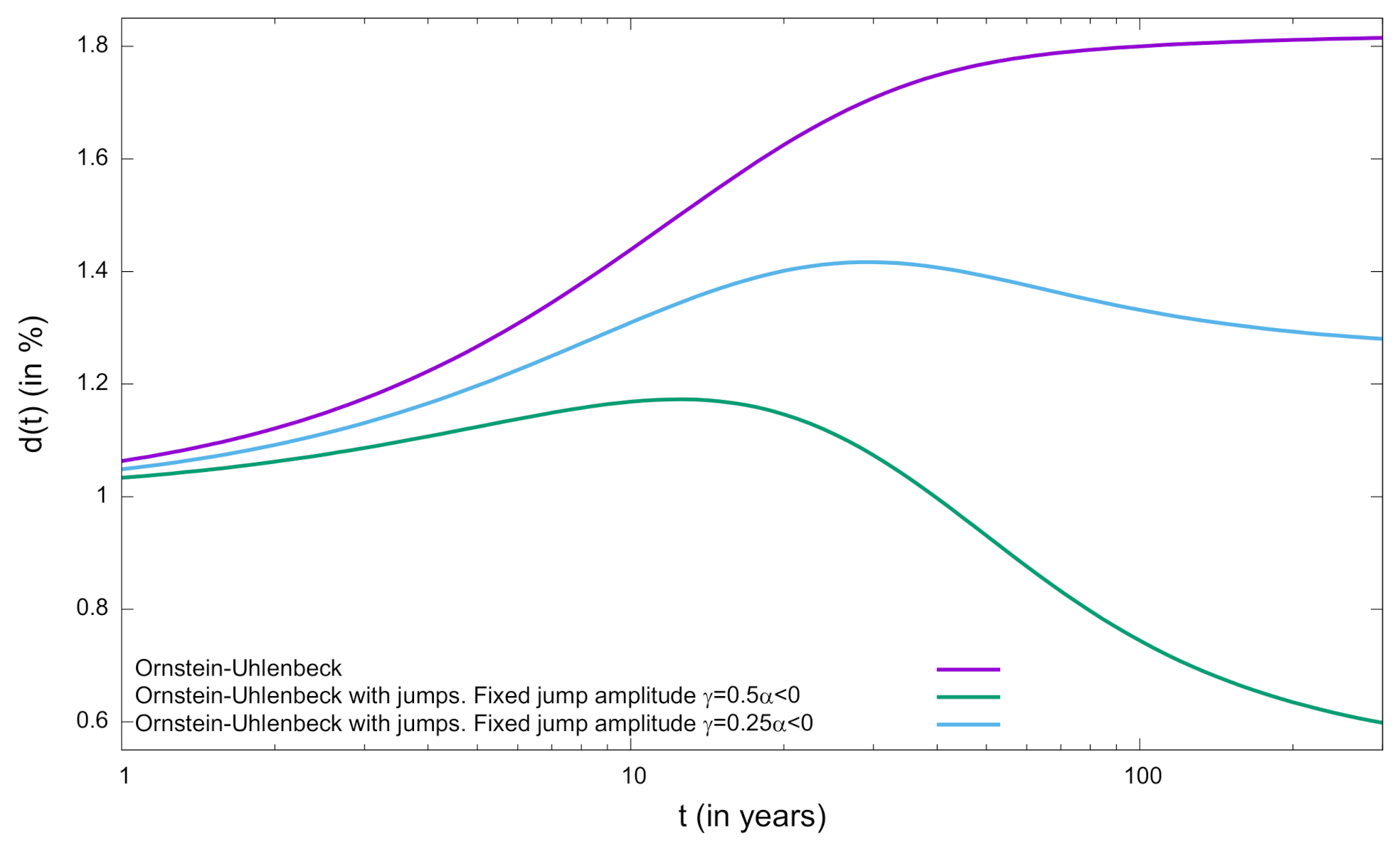
3.2.1. Fixed Jump Amplitudes

Let us first assume that the amplitudes of the discontinuities consist of a series of N fixed values, ${\gamma }_1,\cdots ,{\gamma }_N$ ($N=1,2,3,\cdots$). If these values are equally likely, the jump distribution function is

$$h\left(u\right)=\frac{1}{N}\sum _{j=1}^N\delta (u-{\gamma }_j)\Rightarrow \tilde{h}\left(\theta \right)=\frac{1}{N}\sum _{j=1}^N{e}^{-i\theta {\gamma }_j}.$$

(49)

In this case, the function $\varphi \left(t\right)$ defined in (35) can be written as

$$\begin{array}{c}\hfill \varphi \left(t\right)=-\frac{1}{\alpha N}\sum _{j=1}^N{\int }_0^{(1-e^{-\alpha t})/\alpha }\frac{e^{-{\gamma }_j\xi }}{1/\alpha -\xi }d\xi =\frac{1}{\alpha N}\sum _{j=1}^N{e}^{-{\gamma }_j/\alpha }{\int }_{1/\alpha }^{e^{-\alpha t}/\alpha }\frac{e^{{\gamma }_j\eta }}{\eta }d\eta \\ \hfill =\frac{1}{\alpha N}\sum _{j=1}^N{e}^{-{\gamma }_j/\alpha }\left[Ei\left({\gamma }_i{e}^{-\alpha t}/\alpha \right)-Ei\left({\gamma }_i/\alpha \right)\right],\end{array}$$

(50)

where $Ei(·)$ is the Exponential integral defined as [42]

$$Ei\left(x\right)={\int }_{-\infty }^x\frac{e^{\eta }}{\eta }d\eta .$$

Expanding the integrand we get:

$$\int \frac{e^{\eta }}{\eta }d\eta =ln\eta +\sum _{n=1}^{\infty }\frac{{\eta }^n}{nn!}.$$

Hence

$${\int }_{1/\alpha }^{e^{-\alpha t}/\alpha }\frac{e^{{\gamma }_j\eta }}{\eta }d\eta =-\alpha t-\sum _{n=1}^{\infty }\frac{{({\gamma }_j/\alpha )}^n}{nn!}\left(1-e^{-n\alpha t}\right),$$

and

$$\varphi \left(t\right)=-\left(\frac{1}{N}\sum _{j=1}^N{e}^{-{\gamma }_j/\alpha }\right)t-\frac{1}{\alpha N}\sum _{j=1}^N{e}^{-{\gamma }_j/\alpha }{\psi }_j\left(t\right),$$

(51)

where

$${\psi }_j\left(t\right)\equiv \sum _{n=1}^{\infty }\frac{{({\gamma }_j/\alpha )}^n}{nn!}\left(1-e^{-n\alpha t}\right).$$

(52)

The discount function $D\left(t\right)$, given in Equation (33), now reads

$$D\left(t\right)=D^{\left(0\right)}\left(t\right)exp\left\{-\lambda t\left[1-\frac{1}{N}\sum _{j=1}^N{e}^{-{\gamma }_j/\alpha }\right]+\frac{\lambda }{\alpha N}\sum _{j=1}^N{e}^{-{\gamma }_j/\alpha }{\psi }_j\left(t\right)\right\}$$

(53)

with the jump-free discount $D^{\left(0\right)}\left(t\right)$ given by Equation (34).

Figure 1 shows the effect on the average discount rate $d\left(t\right)$, defined in (3), of the presence of jumps with the simplest possible case when there is only one jump amplitude $\gamma <0$ ($N=1$). In this case, the average discount rate reads (cf. Equations (53) and (50))

$$d\left(t\right)=-\frac{ln{D}^{\left(0\right)}\left(t\right)}{t}+\lambda \left\{1+\frac{exp\left(-\gamma /\alpha \right)}{\alpha t}\left[Ei\left(\gamma e^{-\alpha t}/\alpha \right)-Ei\left(\gamma /\alpha \right)\right]\right\}.$$

(54)

In Figure 1, we assume a jump frequency $\lambda =0.02$ 1/year (1 jump every 50 years) and show how the discount $d\left(t\right)$ changes as a function of time when considering no jumps and negative jumps of size $\left|\gamma \right|/\alpha =0.25$ and 0.5, where $\alpha$ is the reversion to the mean of the OU process (cf. Equation (16)). When considering the case of United States of America [17], it can be shown that small changes in $\gamma <0$ parameter can lead to very sensitive effects to the discount rate, lowering the rate to values close to 1% and lower, even if jumps size are small or very small.

In the long-run, as $t\to \infty$, we see from (51) and (52) that

$$\varphi \left(t\right)\simeq -\left(\frac{1}{N}\sum _{j=1}^N{e}^{-{\gamma }_j/\alpha }\right)t(t\to \infty ),$$

and the discount function can be approximated by Equation (41):

$$D\left(t\right)\simeq e^{-r_{\infty }t},(t\to \infty ),$$

where the long-run discount rate given in Equation (42) now reads

$$r_{\infty }=r_{\infty }^{\left(0\right)}+\lambda \left[1-\frac{1}{N}\sum _{j=1}^N{e}^{-{\gamma }_j/\alpha }\right]$$

(55)

and $r_{\infty }^{\left(0\right)}$ is the jump-free discount rate, Equation (43). Let us also note that $r_{\infty }<r_{\infty }^{\left(0\right)}$ if

$$\frac{1}{N}\sum _{j=1}^N{e}^{-{\gamma }_j/\alpha }>1.$$

(56)

The simplest case, when all jumps have the same amplitude, ${\gamma }_j=\gamma$, reads (cf. Equation (55))

$$r_{\infty }=r_{\infty }^{\left(0\right)}+\lambda \left[1-e^{-\gamma /\alpha }\right].$$

(57)

In this case, if there is a sudden decrease in return ($\gamma <0$) then $r_{\infty }<r_{\infty }^{\left(0\right)}$. Otherwise, an increase of return ($\gamma >0$) implies the increase of the long-run discount ratio, $r_{\infty }>r_{\infty }^{\left(0\right)}$. These results are consistent with condition (44). Figure 2 shows how $r_{\infty }$ change as a function of the scaled dimensionless jump length magnitude $\left|\gamma \right|/\alpha$ where $\alpha$ is the reversion to the mean of the OU process (cf. Equation (16)). Figure 2 shows the opposite effects in the long run discount function for positive and negative jumps when $r_{\infty }^{\left(0\right)}=1.81\%$, which corresponds to the long-run discount rate estimated in Ref. [17] with United States of America (USA) real interest rate ratio datasets. For positive jumps $\gamma >0$, the long-run rate in the case of USA can increase up to 3% with jump amplitudes of size 5% taking place once every 50 years. For negative jumps $\gamma <0$, the long-run discount rates can become negative for jumps amplitudes of only 4%. These results confirm the high sensitivity of the long-run discount rate $r_{\infty }$ when considering jumps.

Another particular case consists in assuming that discontinuities have only two possible amplitudes, which are equal but of opposite signs, that is, ${\gamma }_1=\gamma$ and ${\gamma }_2=-\gamma$. Now (cf. (49))

$$\tilde{h}\left(\theta \right)=cosh(\gamma \theta /\alpha )$$

and the long-run discount rate (42) is

$$r_{\infty }=r_{\infty }^{\left(0\right)}+\lambda \left[1-cosh(\gamma /\alpha )\right].$$

(58)

Note that since $cosh(\gamma /\alpha )>1$ for all values of $\gamma /\alpha$, then $r_{\infty }<r_{\infty }^{\left(0\right)}$. In this example in which return suddenly decreases or increases equally likely by a fixed quantity, discontinuities always reduce the long-run rate, as we have already proved in a previous section. Figure 2 shows that this decrease can be quite sensitive even when jumps amplitudes are relatively small ($r_{\infty }$ can already be negative when jumps sizes are of the order of 5% when considering USA datasets).

3.2.2. Laplacian Jump Amplitudes

As a second example, we suppose that jump amplitudes are not fixed but distributed according to the Laplace (“tent shape”) density:

$$h\left(u\right)=\frac{1}{\sqrt{2}\gamma }{e}^{-\sqrt{2}\left|u\right|/\gamma },$$

(59)

$(\gamma >0)$. In this model, increasing and decreasing jumps are equally likely with zero average discontinuity, $\langle \Delta r\rangle =0$, and $\sigma =\sqrt{\langle \Delta r^2\rangle }=\gamma$. Thus, the parameter $\gamma$ represents the average of absolute values of the amplitude of discontinuities. Bearing in mind that Equation (59) represents a symmetric distribution around $u=0$ we see that the Fourier transform of $h\left(u\right)$ can be written as

$$\tilde{h}\left(\theta \right)=\frac{2}{\gamma \sqrt{2}}{\int }_0^{\infty }{e}^{-u\sqrt{2}/\gamma }cos\left(\theta u\right)du.$$

(60)

When $\theta \in \mathbb{R}$ is real direct integration [42] yields

$$\tilde{h}\left(\theta \right)=\frac{1}{1+{\gamma }^2{\theta }^2/2}.$$

(61)

Suppose, however, that $\theta =i\xi$$(\xi \in \mathbb{R})$ is an imaginary number, in such a case since $cosi\theta =cosh\xi$ the integral in Equation (60) diverges when $\left|\xi \right|\ge \sqrt{2}/\gamma$. We thus have

$$\tilde{h}\left(i\xi \right)=\left\{\begin{array}{cc}\frac{1}{1-{\gamma }^2{\xi }^2/2},\hfill & \left|\xi \right|<\sqrt{2}/\gamma ,\hfill \\ \infty \hfill & \left|\xi \right|\ge \sqrt{2}/\gamma .\hfill \end{array}\right.$$

(62)

For the special case $\xi =-1/\alpha$, we have

$$\tilde{h}(-i/\alpha )=\left\{\begin{array}{cc}1/(1-c^2),\hfill & c<1,\hfill \\ \infty ,\hfill & c\ge 1,\hfill \end{array}\right.$$

(63)

where

$$c\equiv \frac{\gamma }{\alpha \sqrt{2}}$$

(64)

is a dimensionless parameter that combines the average absolute jump $\gamma$ and the strength $\alpha$ of the reversion to the mean of the OU process.

Recall that in terms of the jump-free discount, the discount function is given by (cf. Equation (33))

$$D\left(t\right)=D^{\left(0\right)}\left(t\right)e^{-\lambda [t+\varphi (t\left)\right]}.$$

(65)

where $D^{\left(0\right)}\left(t\right)$ and $\varphi \left(t\right)$ are, respectively, given by Equations (34) and (35). In the Appendix C, we show that for the Laplace density (59), the form and behavior of the discount function depends on the value of the parameter c defined in Equation (64). We have three cases:

1.

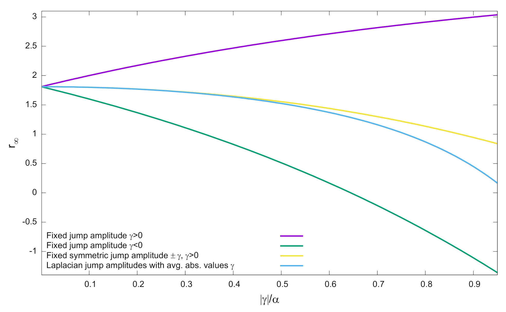
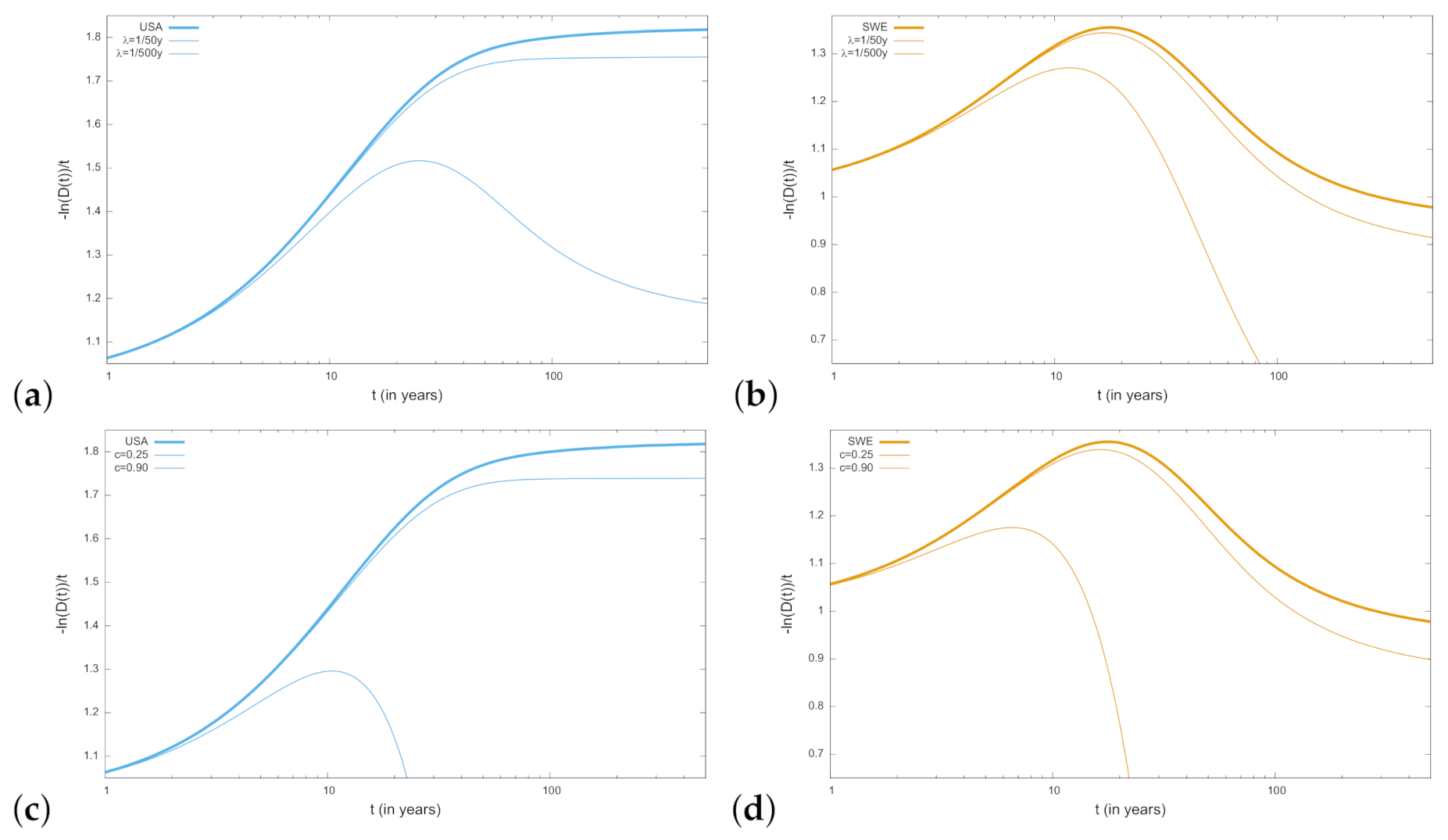
When $c<1$ (i.e., $\gamma <\alpha \sqrt{2}$) we prove in the Appendix C that the function $\varphi \left(t\right)$ is given by

$$\varphi \left(t\right)=-\frac{t}{1-c^2}-\frac{1}{2\alpha }\left[\frac{1}{1-c}ln\left(1-c(1-e^{-\alpha t})\right)+\frac{1}{1+c}ln\left(1+c(1-e^{-\alpha t})\right)\right].$$

(66)

In this case, the discount function is finite and follows from Equation (65) after substituting Equation (66). Figure 3 illustrate this result considering the OU parameters estimated in Ref. [17] while considering different jumps frequencies $\lambda$ and different jumps amplitudes in terms of c. For large values of t, we have

$$\varphi \left(t\right)\simeq -\frac{t}{1-c^2},(t\to \infty ).$$

Since $D^{\left(0\right)}\left(t\right)\simeq e^{-r_{\infty }^{\left(0\right)}t}$ as $t\to \infty$ (cf. Equations (36) and (43)), we finally obtain

$$D\left(t\right)\simeq exp\left\{-\left[r_{\infty }^{\left(0\right)}-\lambda c^2/(1-c^2)\right]t\right\},(t\to \infty ),$$

(67)

and the expression for the long-run rate reads

$$r_{\infty }=r_{\infty }^{\left(0\right)}-\frac{\lambda c^2}{1-c^2}<r_{\infty }^{\left(0\right)},(c<1),$$

(68)

with $r_{\infty }^{\left(0\right)}$ given in Equation (43). In this model, discontinuities reduce the long-run discount rate if $c<1$, which implies that $r_{\infty }$ is finite. That is, when $\gamma <\alpha \sqrt{2}$ and the average of the absolute value of discontinuities is smaller than the strength of the reversion to the mean represented by $\alpha \sqrt{2}$. The behavior of the long-run discount rate $r_{\infty }$ for Laplacian jumps can be compared to the fixed and bounded jumps amplitude case provided in Section 3.2.1. As shown in Figure 2, the behavior is qualitatively similar to the case of two symmetric jumps. The differences among both examples become relevant when $c\to 1^{-}$, being the curve consistent with the critical behavior described in Equation (63).

2.

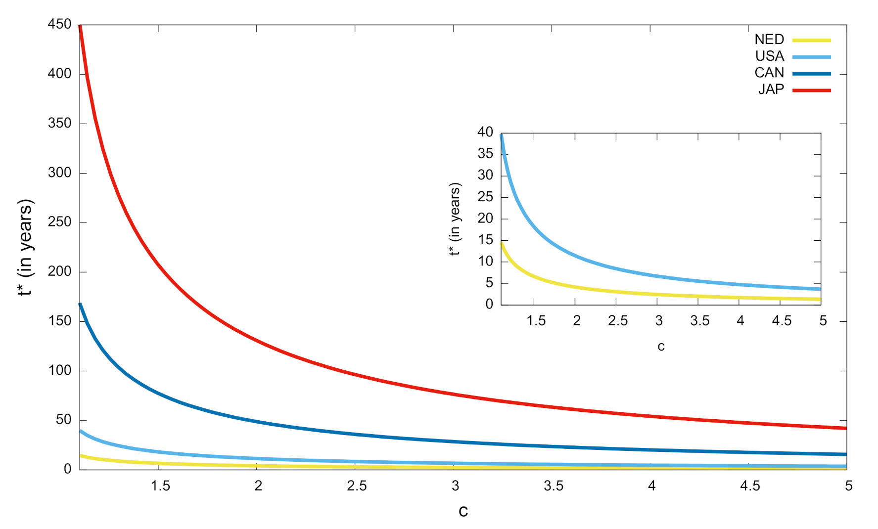
When $c>1$ (i.e., $\gamma >\alpha \sqrt{2}$), we prove in the Appendix C that the discount becomes infinite for times greater than a critical time,

$$D\left(t\right)=\infty ,(t\ge t^{\ast }),$$

(69)

where

$$t^{\ast }=-\frac{1}{\alpha }ln\left(1-\frac{1}{c}\right),$$

(70)

while for $t<t^{\ast }$ the discount function is given as in case (i) above (even though now it has no sense asking for the asymptotic behavior of discount as $t\to \infty$). Figure 4 shows the sensitivity of the critical time with respect to jumps amplitude. We there show that critical time $t^{\ast }$ can become shorter than a year or be strongly reduced as c increases.

3.

For the threshold case $c=1$ (i.e., $\gamma =\alpha \sqrt{2}$), the discount function grows exponentially. Thus, in the Appendix C we show that

$$D\left(t\right)\simeq exp\left\{\frac{\lambda }{2\alpha }{e}^{\alpha t}\right\},(t\to \infty ).$$

(71)

Note that this behavior is not contradictory with our previous results since, as $r_{\infty }^{\left(0\right)}>0$ and

$$1<\frac{2{\alpha }^2}{{\gamma }^2}<1+\frac{\lambda }{r_{\infty }^{\left(0\right)}},$$

$r_{\infty }$ becomes negative, and discount turns into an increasing function for t large enough.

From this case, we conclude that if jump amplitudes are on average smaller than the restoring force toward the normal level ($\gamma <\alpha \sqrt{2}$) jumps reduce the long-run discount rate. However, when jump amplitudes are larger ($\gamma >\alpha \sqrt{2}$), the discount function becomes infinite at a finite time.

3.3. Discount in the Continuous Time Random Walk Formalism

Up to this point, we have dealt with a rate process described by a diffusion process in which there are superimposed finite discontinuities. At one extreme of the model, we find continuous diffusion processes with no discontinuities, which have been developed in our previous works [15,17,26]. At the other extreme, we find a purely discontinuous process where the return starting at some initial value keeps this value during a random interval of time and makes a sudden jump with a random amplitude to a new value, keeps the new value another random time interval, makes another jump, and so on. This is precisely the Continuous Time Random Walk (CTRW) with countless applications in many branches of natural sciences, engineering and economics and social sciences [43,44]. Let us observe that if waiting times between jumps are Poissonian with rate $\lambda$ and independent of the jump amplitudes, then the PDF of the bidimensional process $\left(x\right(t),r(t\left)\right)$—which we denote by $p_0(x,r,t|r_0)$—is described by the integro-differential Equation (14) with $f\left(r\right)=g\left(r\right)=0$

$$\frac{\partial p_0}{\partial t}=-r\frac{\partial p_0}{\partial x}-\lambda p_0(x,r,t|r_0)+\lambda {\int }_{-\infty }^{\infty }h(r-\rho )p_0(x,\rho ,t|r_0)d\rho ,$$

(72)

with the initial condition

$$p_0(x,r,0|r_0)=\delta \left(x\right)\delta (r-r_0).$$

(73)

By Fourier transforming this problem, we easily obtain the expression for the characteristic function $\tilde{p}({\omega }_1,{\omega }_2,t|r_0)$. It reads (this solution can be also obtained from Equation (23) with the values $\alpha =0$ and $k=0$):

$${\tilde{p}}_0({\omega }_1,{\omega }_2,t|r_0)=exp\left\{-i({\omega }_{1}t+{\omega }_2)r_0-\lambda \left[t-\frac{1}{{\omega }_1}{\int }_{{\omega }_2}^{{\omega }_{1}t+{\omega }_2}\tilde{h}\left(\theta \right)d\theta \right]\right\}.$$

(74)

The marginal distribution of the return, ${\tilde{p}}_0({\omega }_2,t|r_0)$, is obtained from (74) after setting ${\omega }_1=0$:

$${\tilde{p}}_0({\omega }_2,t|r_0)=exp\left\{-i{\omega }_2{r}_0-\lambda t\left[1-\tilde{h}\left({\omega }_2\right)\right]\right\},$$

(75)

and the return variance reads ${\sigma }_0^2\left(t\right)=\lambda \mu t$, where $\mu =-{\tilde{h}}^{\prime \prime }\left(0\right)$ is the jump second moment.

The discount function is obtained by setting ${\omega }_1=-i$ and ${\omega }_2=0$ in the joint characteristic function (74). For the CTRW model, this yields

$$D_0\left(t\right)=exp\left\{-r_{0}t-\lambda \left[t+{\varphi }_0\left(t\right)\right]\right\},$$

(76)

where

$${\varphi }_0\left(t\right)=\frac{1}{i}{\int }_0^{-it}\tilde{h}\left(\theta \right)d\theta =-{\int }_0^t\tilde{h}(-i\xi )d\xi .$$

(77)

Equation (76) is the expression of the discount function when rates are modeled by a Markovian CTRW with a general jump density $h\left(u\right)$.

In the special case of Laplacian jumps $\tilde{h}(-i\xi )$ (cf. Equation (62))

$$\tilde{h}\left(i\xi \right)=\left\{\begin{array}{cc}\frac{1}{1-{\gamma }^2{\xi }^2/2},\hfill & \left|\xi \right|<\sqrt{2}/\gamma ,\hfill \\ \infty \hfill & \left|\xi \right|\ge \sqrt{2}/\gamma .\hfill \end{array}\right.$$

(78)

For times such that $t<\sqrt{2}/\gamma$, we see from Equation (77) that $\xi <t<\sqrt{2}/\gamma$, hence

$${\varphi }_0\left(t\right)=-{\int }_0^t\frac{d\xi }{1-{\gamma }^2{\xi }^2/2}=\frac{1}{\gamma }\left[-ln\left(1-\gamma t/\sqrt{2}\right)+ln\left(1+\gamma t/\sqrt{2}\right)\right].$$

In this case, the discount function reads

$$D_0\left(t\right)={\left(\frac{1+\gamma t/\sqrt{2}}{1-\gamma t/\sqrt{2}}\right)}^{\lambda /\gamma }{e}^{-(r_0+\lambda )t},(t<\sqrt{2}/\gamma ).$$

(79)

On the other hand, if $t>\sqrt{2}/\gamma$, we can write

$${\varphi }_0\left(t\right)=-\left[{\int }_0^{\sqrt{2}/\gamma }\tilde{h}(-i\xi )d\xi +{\int }_{\sqrt{2}/\gamma }^t\tilde{h}(-i\xi )d\xi \right].$$

However, due to Equation (78), the second integral is infinite, hence ${\varphi }_0\left(t\right)=-\infty$ and

$$D_0\left(t\right)=\infty ,(t>\sqrt{2}/\gamma ).$$

(80)

Therefore, for the CTRW model with Laplacian jumps, the discount function becomes infinite in the finite time $t^{\ast }=\sqrt{2}/\gamma$.

4. Discussion

In a series of recent works [15,16,17,26,30], we have analyzed the process of discounting using mostly methods borrowed from non-equilibrium statistical physics and stochastic processes. In these works, we have considered three of the most popular stochastic models for the dynamics of interest rates: Ornstein–Uhlenbeck [27], Feller [28], and log-normal [29] processes, which are also very relevant in statistical physics. However, we are interested in real rates (that is, nominal rates corrected by inflation), which can be negative even during prolonged periods of time [15,17] and, since Feller and log-normal models deal exclusively with positive quantities, this leads to the Ornstein–Uhlenbeck (OU) process as the only model with mean reversion and allowing for negative rates. The Ornstein–Uhlenbeck (OU) model is the only one that allows for negative rates while still considering simplest (and linear) mean reversion towards a normal interest rate. Mean-reversion assumes that the interest rate follows a stationary process and this can be considered as a limitation when the model is contrasted with empirical data.

The work presented here continues with such an undertaking, but we go one step further and assume that, in addition to diffusive and continuous behavior, the sample paths of real rates $r\left(t\right)$ also exhibit discontinuities. That is, we will model rates by a jump-diffusion process as the economic evolution is known to occasionally have sudden bursts that hardly adjust to continuous diffusion-like evolution. We have thus wanted to elucidate the effect on the long-run discount of discontinuities that reflect the high-risk events that might occur in the future.

We have obtained a very general formula of the discount function for processes that combine an Ornstein–Uhlenbeck (OU) dynamics with the presence of Poissonian jumps with frequency $\lambda$ (see also the Feller process with jumps in [13]). Equation (33) shows this key result. Two almost immediate questions are: how this general formula behaves for very long times? Additionally, which is the resulting long-run discount rate $r_{\infty }$? Thus, if $\tilde{h}\left(\theta \right)$ is the jump characteristic function, we have proved that as long as $\tilde{h}(-i/\alpha )$ exists, one obtains a value for $r_{\infty }$. Otherwise, the discount becomes infinite for a finite time horizon. An infinite discount is indeed catastrophic for the economy because it implies that any future value is zero. Furthermore, in case that $\tilde{h}(-i/\alpha )>1$, the addition of jumps to the model results into a decrease of $r_{\infty }$ (cf. Equations (43) and (44)). This latter case entails a call for a more immediate action to climate change and it applies to those processes with symmetric jump amplitude. The obtention of lower long-run discount rates $r_{\infty }$ for symmetric jumps amplitude is of particular importance, as it deepens in the idea already suggested by the OU process with no sudden jumps. That is to say, the fact that bounded unbiased uncertainty, no matter whether continuous or not, increases the urgency for immediate action.

To go deeper in evaluating the effect of discontinuities, we have gone through three different scenarios. The simplest case refers to the existence of a fixed jumps amplitude. We have been able to obtain the exact formula for the discount, which is represented in Figure 1 by considering the parameters of the OU process for United States of America [17] for a single negative jump $\gamma$. We there show that even by considering a frequency $\lambda$ of one jump every 50 years and small jumps ($\gamma =0.5\alpha$) the effect is more than evident. As expected, sudden negative returns represent a quicker decrease in the discount function. Negative jumps of $5\%$ return size (due to catastrophic news such as the COVID-19 outbreak) can already lead $r_{\infty }$ to negative values, which in practice is telling us that immediate actions with strong investment are unavoidable to face, even if they are unknown, climate effects in the future (see Figure 2). In contrast, the assumption of having future sudden positive returns—due, for instance, to positive news or a major technological breakthrough—increments $r_{\infty }$, thus releasing pressure for taking action rapidly. It is, however, important to mention that the increment is lower than the decrement observed for negative jumps of the same size (see Figure 2).

A more sophisticated scenario is to consider the possibility of having two jumps of the same amplitude, but of opposite signs. This symmetric scenario also allows us to obtain the discount function, and this case always lowers the rate because of its symmetry. In the case of USA, as can also be shown in Figure 2, this drives $r_{\infty }$ from 1.8% to 1% with jump amplitude $\gamma =5\%$ and frequency $\lambda =(1/50){\mathrm{year}}^{-1}$.

While keeping the same number of parameters (so it does not provide further complexity in data calibration), but considering a symmetric and continuous distribution of jumps amplitude (Laplace density), it is possible to provide a third scenario. This case interestingly contrasts to the case of two fixed and symmetric jumps. Laplacian jumps brings up two different discount solutions depending on the value of $c=\gamma /\alpha \sqrt{2}$. The jump size average $\gamma$ must be compared to the mean-reversion intensity $\alpha$ (cf. Equation (64)). If $c<1$, it is possible to obtain an analytical formula of the discount function, which is carefully explored in Figure 3 with the OU estimated parameters with real interest rate datasets from USA and Sweden [17]. We there extend the analysis by exploring the effect of different values for jumps frequency $\lambda$ and scaled jump amplitude c. However, when $c>1$, the discount function becomes infinite for a critical time $t^{\ast }$. Figure 4 shows that the critical time $t^{\ast }$ is quite sensitive to jumps amplitude size in a wide variety of cases and $t^{\ast }$ can become rather small, even for small jump amplitudes (For instance, few years, less than a decade, with jumps amplitude size about 7%, if we consider OU parameter from the case of USA).

Finally, it is also possible to obtain the discount function if we disregard the diffusion contribution. This scenario corresponds to the Continuous Time Random Walk and the results when assuming Laplacian jumps amplitudes are different depending on the critical time $\sqrt{2}/\gamma$. At short times, when $t<\sqrt{2}/\gamma$, the discount function decreases exponentially (cf. Equation (79)). However, as $t>\sqrt{2}/\gamma$, the discount function becomes infinite.

5. Conclusions

The main results of this paper are summarized in

Table 1. Summary of the results proved in Section 3. The Ornstein–Uhlenbeck diffusion process already shows that the presence of noise ($k\ne 0$) reduces the long-run discount rate $r_{\infty }^{\left(0\right)}$. The inclusion of Poissonian jumps with specific scenarios leads to several discount functions $D\left(t\right)$ and several long-run discount rate $r_{\infty }$.

Model	Discount
Main definitions	Discount function:
$dx/dt=r$	$D\left(t\right)=\mathbb{E}\left[exp\left(-{\int }_0^{t}r\left(t^{\prime }\right)d{t}^{\prime }\right)\right]$
$dr/dt=f\left(r\right)+g\left(t\right)\xi \left(t\right)+n\left(t\right)$	Discount rate: $lnD\left(t\right)/t$
	Long-run discount rate:
	$r_{\infty }={lim}_{t\to \infty }lnD\left(t\right)/t$
Ornstein–Uhlenbeck (OU)
$dr/dt=-\alpha (r-m)dt+k\xi \left(t\right)$	$r_{\infty }^{\left(0\right)}=m-k^2/\left(2{\alpha }^2\right)$
OU and Poissonian jumps
$dr/dt=-\alpha (r-m)dt+k\xi \left(t\right)+n\left(t\right)$
$n\left(t\right)={\sum }_j{\gamma }_j\delta (t-t_j)$
Jumps size PDF $h\left({\gamma }_j\right)$
Poissonian $\tau =t_{i+1}-t_i$ time interval PDF
$\psi \left(\tau \right)=\lambda e^{-\lambda \tau }$
If $\tilde{h}(-i/\alpha )$ is finite	$r_{\infty }=r_{\infty }^{\left(0\right)}+\lambda \left[1-\tilde{h}(-i/\alpha )\right]$
If $\tilde{h}(-i/\alpha )$ is finite and $\tilde{h}(-i/\alpha )>1$	$r_{\infty }<r_{\infty }^{\left(0\right)}$
If $\tilde{h}(-i/\alpha )$ is finite and jumps are symmetric	$r_{\infty }<r_{\infty }^{\left(0\right)}$
If jumps have two fixed amplitudes $\pm \gamma$	$r_{\infty }=r_{\infty }^{\left(0\right)}+\lambda [1-cosh(\gamma /\alpha )]<r_{\infty }^{\left(0\right)}$
Laplacian jumps with absolute jump average $\gamma$
If $0<\gamma <\alpha \sqrt{2}$	$r_{\infty }=r_{\infty }^{\left(0\right)}-\frac{\lambda }{2{\alpha }^2/{\overline{\gamma }}^2-1}<r_{\infty }^{\left(0\right)}$
If $\gamma >\alpha \sqrt{2}$	Not defined
	Critical explosive time
If jumps have one-fixed increasing amplitude	$r_{\infty }=r_{\infty }^{\left(0\right)}+\lambda \left(1-e^{-\left|\gamma \right|/\alpha }\right)>r_{\infty }^{\left(0\right)}$
If jumps have one-fixed decreasing amplitude	$r_{\infty }=r_{\infty }^{\left(0\right)}+\lambda \left(1-e^{\left|\gamma \right|/\alpha }\right)<r_{\infty }^{\left(0\right)}$
If jumps have two-fixed amplitudes $\pm \gamma$	$r_{\infty }=r_{\infty }^{\left(0\right)}+\lambda [1-cosh(\gamma /\alpha )]<r_{\infty }^{\left(0\right)}$
Continuous Time Random Walk
$dr/dt=n\left(t\right)$
Laplacian jumps with absolute jump average $\gamma$	Not defined
	Critical explosive time $t^{\ast }=\sqrt{2}/\gamma$

. Let us recall that the chief objective of the present work is to contribute to the mathematical modeling of discounting, within the context of environmental economics and climate action, by considering extreme situations or outliers. Although Martin Weitzman has already introduced the effect of fat tails in the economic evolution [34,35], our approach here is more dynamical and it is based not on fat tails, but on the addition of discontinuities in the economic time evolution. As we have shown such discontinuities may result, under certain conditions, into an infinite discount, confirming what Weitzman foresaw a few years ago. Let us emphasize that our approach (being complementary to that of Weitzman) provides a very general mathematical framework which allows for direct computation which can lead to future research in for instance option pricing by means of the martingale analysis and the characteristic function of the process.

We have also explored specific scenarios that show that discontinuities due to unexpected shocks (even if they represent downside shocks such as epidemics or a climate disaster or upside shocks due, for instance, to a new technological breakthrough) can severely affect current estimates of economic variables such as the long-run discount rate. Changes on this economic variables are shown to be strong enough to influence current decision mechanisms on whether and in which degree we shall take action today to face climate change.

We finally would like to stress the fact that that we here have wanted to include extreme and infrequent events to the rate process. The most natural choice to capture these events is to consider the addition of a Poisson jump process to an underlying diffusion process. However, there are other ways to incorporate a more generic class of jumps, which allows both frequent and infrequent jumps [45,46]. This generalization could lead to new and interesting theoretical results for the discount function that definitely would deserve careful attention and can drive new promising research avenues.

References

- Stern, N. The Economics of Climate Change: The Stern Review; Cambridge University Press: Cambridge, UK, 2006. [Google Scholar]
- Nordhaus, W.D. The Stern Review on the economics of climate change. J. Econ. Lit. 2007, 45, 687–702. [Google Scholar] [CrossRef]
- Nordhaus, W.D. Critical assumptions in the Stern Review on Climate Change. Science 2007, 317, 201–202. [Google Scholar] [CrossRef] [PubMed]
- Stern, N. Ethics, Equity and the Economics of Climate Change. Paper 1: Science and Philosophy. Econ. Philos. 2014, 30, 397–444. [Google Scholar] [CrossRef]
- Stern, N. Ethics, Equity and the Economics of Climate Change. Paper 2: Economics and Politics. Econ. Philos. 2014, 30, 445–501. [Google Scholar] [CrossRef]
- Heal, G.M.; Millner, A. Agreeing to disagree on climate policy. Proc. Natl. Acad. Sci. USA 2014, 111, 3695–3698. [Google Scholar] [CrossRef]
- Ramsey, F.P. A mathematical theory of saving. Econ. J. 1928, 38, 543–559. [Google Scholar] [CrossRef]
- Arrow, K.J.; Cropper, M.L.; Gollier, C.; Groom, B.; Heal, G.M.; Newell, R.G.; Nordhaus, W.D.; Pindyck, R.S.; Pizer, W.A.; Portney, P.R.; et al. Determining Benefits and Costs for Future Generations. Science 2013, 341, 349–350. [Google Scholar] [CrossRef]
- Heath, D.; Jarrow, R.; Morton, A. Bond pricing and the term structure of interest rates: A new methodology for contingent claims valuation. Econom. J. Econom. Soc. 1992, 60, 77–105. [Google Scholar] [CrossRef]
- Vasicek, O. An equilibrium characterization of the terms structure. J. Financ. Econ. 1977, 5, 177–188. [Google Scholar] [CrossRef]
- Cox, J.C.; Ingersoll, J.E.; Ross, S.A. A theory of the term structure of interest rates. Econometrica 1985, 53, 385–407. [Google Scholar] [CrossRef]
- Dothan, L.U. On the term structure of interest rates. J. Financ. Econ. 1978, 6, 59–69. [Google Scholar] [CrossRef]
- Ahn, C.M.; Thompson, H.E. Jump-diffusion processes and the term structure of interest rates. J. Finance 1988, 43, 155–174. [Google Scholar] [CrossRef]
- Brigo, D.; Mercurio, F. Interest Rate Models—Theory and Practice; Springer: Berlin/Heidelberg, Germany, 2006. [Google Scholar]
- Farmer, J.D.; Geanakoplos, J.; Masoliver, J.; Montero, M.; Perelló, J. Discounting the Distant Future; Cowles Foundation Discussion Paper no. 1951; University of Yale: New Haven, CT, USA, 2014. [Google Scholar]
- Farmer, J.D.; Geanakoplos, J.; Masoliver, J.; Montero, M.; Perelló, J.; Richiardi, M.G. Discounting the distant future: What do historical bond prices imply about the long term discount rate? J. Math. Econ. 2020, submitted. [Google Scholar]
- Perelló, J.; Montero, M.; Masoliver, J.; Farmer, J.D.; Geanakoplos, J. Statistical analysis and stochastic interest rate modeling for valuing the future with implications in climate change mitigation. J. Stat. Mech. 2020, 2020, 0432110. [Google Scholar] [CrossRef]
- Weitzman, M.L. Why the far-distant future should be discounted at its lowest possible rate? J. Environ. Econ. Manag. 1998, 36, 201–208. [Google Scholar] [CrossRef]
- Gollier, C.; Koundouri, P.; Pantelidis, T. Declining discount rates: Economic justifications and implications for the long-run policy. Econ. Policy 2008, 23, 757–795. [Google Scholar] [CrossRef]
- Newell, R.; Pizer, N. Discounting the Distant Future: How much do uncertain rates increase valuations? J. Environ. Econ. Manag. 2003, 46, 52–71. [Google Scholar] [CrossRef]
- Farmer, J.D.; Geanakoplos, J. Hyperbolic Discounting Is Rational: Valuing the Far Future with Uncertain Discount Rates; Cowles Foundation Discussion Paper no. 1719; University of Yale: New Haven, CT, USA, 2009. [Google Scholar] [CrossRef]
- Geanakoplos, J.; Sudderth, W.; Zeitouini, O. Asymptotic behavior of stochastic discount rate. Indian J. Stat. 2014, 76A, 150–157. [Google Scholar] [CrossRef]
- Cox, C.; Ingersoll, J.E.; Ross, S.A. A re-examination of the traditional hypothesis about the term structure of interest rates. J. Finance 1981, 35, 769–799. [Google Scholar] [CrossRef]
- Gilles, C.; Leroy, S.F. A note on the local expectation hypothesis. J. Finance 1986, 41, 975–979. [Google Scholar] [CrossRef]
- Piazzesi, M. Affine term structure models. In The Handbook of Financial Econometrics; Sahala, Y.A., Hansen, M.P., Eds.; Elsevier: Amsterdam, The Netherlands, 2009; pp. 691–766. [Google Scholar]
- Farmer, J.D.; Geanakplos, J.; Masoliver, J.; Montero, M.; Perelló, J. Value of the future: Discounting in random environments. Phys. Rev. E 2015, 91, 052816. [Google Scholar] [CrossRef]
- Uhlenbeck, G.E.; Ornstein, L.S. On the theory of Brownian Motion. Phys. Rev. 1930, 36, 823–841. [Google Scholar] [CrossRef]
- Feller, W. Two singular diffusion processes. Ann. Math. 1951, 54, 173–182. [Google Scholar] [CrossRef]
- Osborne, M.F.M. Brownian motion in the stock market. Oper. Res. 1959, 7, 145–173. [Google Scholar] [CrossRef]
- Masoliver, J. The value of the distant future: The process of discount in random environments. Estud. Econ. Aplicada 2019, 37. [Google Scholar] [CrossRef]
- Gardiner, C.W. Handbook of Stochastic Methods; Springer: Berlin/Heidelberg, Germany, 1985. [Google Scholar]
- Merton, R.C. Option pricing when underlying stock returns are discontinuous. J. Financ. Econ. 1976, 3, 125–144. [Google Scholar] [CrossRef]
- Kou, S.G. A jump-diffusion model for option pricing. Manag. Sci. 2002, 48, 1086–1101. [Google Scholar] [CrossRef]
- Weitzman, M.L. On modeling and interpreting the economics of catastrophic climate change. Rev. Econ. Stat. 2009, 91, 1–19. [Google Scholar] [CrossRef]
- Weitzman, M.L. Fat-tailed uncertainty in the economics of catastrophic climate change. Rev. Environ. Econ. Policy 2011, 5, 275–292. [Google Scholar] [CrossRef]
- Posner, R.A. Catastrophe: Risk and Response; Oxford University Press: Oxford, UK, 2004. [Google Scholar]
- Susnstein, C.R. Worst-Case Scenarios; Harvard University Press: Cambridge, MA, USA, 2007. [Google Scholar]
- Masoliver, J.; Weiss, G.H. Some first passage time problems for shot noise processes. J. Stat. Phys. 1988, 50, 377–382. [Google Scholar] [CrossRef]
- Masoliver, J.; Weiss, G.H. First passage time statistics for some stochastic processes with superimposed shot noise. Phys. A Stat. Mech. Appl. 1988, 149, 395–405. [Google Scholar] [CrossRef]
- Masoliver, J. Random Processes, First-Passage and Escape; World Scientific: Singapore, 2018. [Google Scholar]
- Courant, R.; Hilbert, D. Methods of Mathematical Physics; Wiley: New York, NY, USA, 1989. [Google Scholar]
- Gradshteyn, I.S.; Ryzhik, I.M. Table of Integrals, Series and Products; Academic Press: San Diego, CA, USA, 2007. [Google Scholar]
- Kutner, R.; Masoliver, J. The continuous time random walk, still trendy: Fifty-year history, state of art and outlook. Eur. Phys. J. B 2017, 90, 50. [Google Scholar] [CrossRef]
- Masoliver, J.; Montero, M.; Perelló, J.; Weiss, G.H. The continuous time random walk formalism in financial markets. J. Econ. Behav. Organ. 2006, 61, 577–598. [Google Scholar] [CrossRef]
- Madan, D.B.; Seneta, E. The Variance Gamma (V.G.) model for share market returns. J. Bus. 1990, 63, 511–524. [Google Scholar] [CrossRef]
- Eberlein, E.; Keller, U. Hyperbolic distributions in finance. Bernoulli 1995, 1, 281–299. [Google Scholar] [CrossRef]