1. Introduction
In past years, many popular and topical MCDM (multiple-criteria decision making) methods have been proposed by researchers, such as AHP (Analytic Hierarchy Process) [
1], TOPSIS (Technique for Order of Preference by Similarity to Ideal Solution) [
2], ELECTRE (Elimination and Choice Expressing Reality) [
3], VIKOR (VlseKriterijumska Optimizacija I Kompromisno Resenje) [
4], TODIM (Tomada de Decisão Iterativa Multicritério) [
5], PROMETHEE (Preference Ranking Organization Method for Enrichment Evaluations)[
6], GDM (Grey Decision Making) [
7], and SWARA (Step-wise Weight Assessment Ratio Analysis) [
8].
In general, the steps taken in MCDM to solve a practical problem can be divided into three parts [
9].
The first step is to obtain decision information, including a criterion weight vector
and a matrix of scores for alternatives, as follows:
where
is the normalized value for
with respect to criterion
.
The second step is to aggregate information
by a certain approach, and most MCDM methods use the following method:
The last step is to sort alternatives by the and select the best alternative.
In the above process, how to determine the weights of criteria is a crucial problem [
10]. Generally, limited knowledge makes it difficult for decision makers (DMs) to directly specify the weights. At present, some weighting methods based on DMs’ preferences have been proposed. Among them, the AHP method, generating the subjective weight of each item by comparing all criteria in pairs, is the most extensively used one [
11]. However, if the number of criteria is large, massive pairwise comparisons will increase the complexity of problems and the inconsistency of expert judgments. To address the challenges of AHP, Rezaei [
12] proposed a new technique based on structured pairwise comparisons, named the Best Worst Method (BWM). In the BWM, only reference comparisons are necessary. Specifically, DMs need to first select the best and worst criteria as benchmarks or references, and then express their preference for the best one over the remaining items and the remaining items over the worst one using a number between 1 and 9, finally obtaining the optimal weights of criteria by solving a max–min nonlinear mathematical model. Compared to AHP methods, the BWM requires fewer pairwise comparisons and produces more reliable results with higher consistency [
13]. However, when the pairwise comparisons are not fully consistent, the min–max nonlinear model will produce multiple optimal solutions. To overcome this disadvantage, Rezaei [
14] transformed this model into a linear one to provide a unique solution. Given the advantages of the BWM, it has been combined with other MCDM methods without a weight derivation process, such as TODIM [
15], VIKOR [
16], TOPSIS [
17], etc., and has been widely applied in many areas.
In some situations, the decision environment in the real world is complex and fast-changing. Limited knowledge and experience mean that DMs cannot give crisp pairwise comparison values for some criteria [
18]. To address this issue, researchers extended the BWM to the fuzzy environment by describing DMs’ preferences with various fuzzy information types, such as fuzzy sets [
19], intuitionistic fuzzy sets [
20], interval type-2 fuzzy sets [
21], probabilistic hesitant fuzzy sets [
22], Z-numbers [
23], rough fuzzy sets [
24], etc. Although the fuzzy extensions of the BWM can handle the ambiguity and uncertainty of expert judgement, the collection of DMs’ preferences in these methods is still based on the assumption that DMs are familiar with all criteria [
25]. However, sometimes, the DMs do not have enough time or energy to study all criteria before making a decision, and they cannot express the preference relation between some criteria, even with fuzzy information. For example, in the case of selecting a suitable car, there are many criteria that consumers need to take into consideration. Some criteria are probably known to consumers, like price, style, brand, fuel consumption, warranty, and so on. Some criteria may not be common for consumers but still important, such as ABS (anti-lock braking system), wheelbase (the distance between the front and back wheels of a car or other vehicle; the longer the wheelbase, the better the driving stability of the vehicle), and maximum torque (this determines the acceleration and climbing performance of the car). In this situation, as a first-time buyer, after looking up and studying the related information about cars, he/she may give high marks for a wheelbase length greater than 3000 and low marks for a wheelbase length lower than 2400. However, the buyer may not give the right answer about the proportion of the wheelbase in the evaluation of the car. If some unfamiliar but actually important criteria are abandoned, it may cause a certain degree of deviation in decision making. Thus, the DM must make a decision quickly with all criteria (both familiar and unfamiliar) taken into consideration.
In these cases, the weights of unfamiliar criteria cannot be determined by the aforementioned BWM method. Therefore, the main question in this study is, when the DMs have no knowledge of certain criteria, how do we determine the weights of these unfamiliar criteria with minimum risk?
Entropy theory is an efficient tool to deal with decision-making problems in uncertain environments. Entropy is a measure of information uncertainty [
26]. The maximum entropy principle is to maintain maximum uncertainty to ensure minimum risk. Applications of the maximum entropy principle are everywhere [
27]. For example, it is often said, ‘Do not put all your eggs in one basket’. This choice keeps to the principle of maximum entropy, so the risks of decision making are minimized. According to this principle, when predicting the probability distribution of a random event, the prediction result should satisfy all known conditions, and any subjective assumptions about unknown information should be avoided. In this case, the probability distribution is the most uniform and the prediction risk is the smallest. Therefore, for calculating the weights of unfamiliar criteria, the principle of maximum entropy can be adopted to ensure objectivity of the results.
Based on the above analysis, this paper introduces the maximum entropy principle into the BWM method to assign weights for the unfamiliar criteria. The main contributions of this paper are as follows. Firstly, we propose a novel MCDM method named BW-MaxEnt, and we demonstrate the steps of this method to resolve the problem of criterion weights. The BW-MaxEnt method can determine the weights of unfamiliar criteria with minimum risk to ensure the reliability of decision making. Secondly, we prove that the model based on BW-MaxEnt can be converted into a convex optimization problem with an overall optimal solution, which shows the rationality of the proposed model. Finally, several numerical examples and a real-world application are executed to illustrate the effectiveness and superiority of the proposed BW-MaxEnt method.
The rest of this study is organized as follows. In
Section 2, we provide an overview of the BWM and the principle of maximum entropy. In
Section 3, BW-MaxEnt is proposed. In
Section 4, to make BW-MaxEnt more comprehensible, we apply BW-MaxEnt to a real-world problem: the procurement of GPU workstations. Conclusions and suggestions for future research directions are presented in
Section 5.
3. BW-MaxEnt
With the increasingly rapid pace of modern life, it is more important for people to make decisions quickly according to their experience and limited knowledge. It becomes uneconomical to put so much energy and time into gathering information and doing research about criteria for a small decision. DMs need to make decisions quickly after scanning the relevant information. In this situation, the BWM is not suitable. For instance, in the case of buying a camera, the decision criteria are
: price,
: weight, and
: pixel count. Supposed the customer is not familiar with pixels and his preference information is
. The model for BWM is shown in the following:
It is easy to prove that the model (8) has infinite optimal solutions. We can obtain an optimal solution of . However, this is an absurd solution as it assigns 1 to the weight of criterion , which is not compared.
MaxEnt is a method that focuses on the practical information. However, some information is difficult to obtain, and DMs need to make judgments based on their own experience and preference. Sometimes, results generated by MaxEnt are unrealistic and unexplainable. Therefore, we propose an integrative method based on BWM and MaxEnt.
3.1. The Step of BW-MaxEnt
Here, we describe the steps of BW-MaxEnt, which comprises seven steps.
Figure 1 illustrates the process of BW-MaxEnt.
- Step 1.
Determine the criteria of the decision.
Summon all DMs and clarify the issues to them. All DMs are free to come up with all possible criteria that have an influence on the evaluation results. Suppose there are altogether -many criteria proposed, and they can be represented as a set .
- Step 2.
Select the familiar criteria.
The DM will be asked to choose criteria that they are familiar with. Suppose that -many criteria are selected, which can be represented as a set . is a subset of .
- Step 3.
Choose the best and worst criteria.
The DM is asked to select the best (most important) criterion () and the worst (least important) criterion () from . It is important to note that only the criteria are considered and not the values of the criteria.
- Step 4.
Make comparisons between the best criterion and all the other criteria.
The DM needs to determine their preference for the best criterion over all the other criteria using a number ranging from 1 to 9. The comparison results of Best-to-Others (BO) can be represented with a vector:
where
indicates the preference for the best criterion over criterion
.
- Step 5.
Make comparisons between each of the other criteria and the worst criterion.
Similarly, the resulting Others-to-Worst (OW) vector would be
where
indicates the preference of the criterion
, over the worst criterion.
- Step 6.
Determine the confidence score.
The DM is asked to give a confidence score for the result of the comparison. is within the range from 0 to 1.
- Step 7.
Establish the mathematical model.
Minimizing the maximum absolute difference
and maximizing the weight entropy
are taken as objective functions. Considering the non-negative and sum-to-one constraints of the weights, the mathematical model is as follows:
where
; when
, Problem (9) degenerates to Problem (2).
Compared with BWM, the model for BW-MaxEnt is a multiobjective programming problem. On the one hand, the absolute difference between the decision preference and ratio of weights is considered, which means that the results become more in line with the expectations of DMs [
12]. On the other hand, by employing the objective function for MaxEnt, we solve the problem of assigning weights to unknown criteria. This also improves the robustness and stability of decision making [
35].
3.2. BW-MaxEnt and Convex Optimization Problems
Because Problem (9) is difficult to solve and could result in multiple optimal solutions, instead of minimizing the maximum value among the set of minimizing maximum absolute differences
, we minimize the maximum among the set
and remove the absolute value symbol in the inequality constraints. Then, the problem can be formulated as follows:
Next, we prove that Problem (10) is a convex optimization problem. For a convex optimization problem, any locally optimal point is also globally optimal [
36]. There are several sophisticated methods to solve convex optimization problems effectively, like the Interior-point method [
37], Subgradient method, and Bundle method [
38].
Theorem 1. If the optimization problem satisfies the following conditions, it is a convex optimization problem [
39]:
- (1)
The feasible region is convex;
- (2)
The objective functionis convex.
According to Theorem 1, if we prove that the feasible region and objective function of Problem (10) are convex, then Problem (10) is a convex optimization problem.
Theorem 2. If a set is the intersection of a finite number of linear inequalities and equalities, the set is a polyhedron. A polyhedron is a convex set [
36]
and can be represented as follows: Firstly, according to Theorem 2, the feasible region of Problem (10) is a polyhedron because its equality constraint is affine and its inequality constraints are linear.
Then, for any
,
, the objective function of Problem (10) is twice differentiable and its Hessian matrix
exists at each point in its feasible region, as follows.
is the
th principal minor of
.
is the determinant of
.
For a problem with more than three criteria, ; for , , so . It can thus be obtained that all minors of are positive. So, is positive definite, and the objective function of Problem (9) is convex. Finally, according to Theorem 1, Problem (10) is therefore a convex optimization problem.
3.3. Consistency and Robust Analysis
By solving Problem (10), the optimal weights
, absolute differences
, and entropy
are obtained. Although
can be regarded as an indicator of the consistency of the comparisons, it does not provide a standard for different comparison scales. Rezaei [
12] proposed a method that applies
to calculate the consistency ratio (CR), and
can be calculated as follows.
Then, he used the maximum values
as a consistency index (CI), which is shown in
Table 1.
Finally, the CR can be calculated as follows
3.4. Numerical Examples
Example 1. This simple example involves a customer who wants to buy a cell phone for himself but is not familiar with all the parameters of the mobile phone. The main decision criteria can be:
price,: style,: camera, and : processor.Table 2shows the vectors of comparison results for the customer. The second line is the BO vector, and the third line is the OW vector.is the best criterion, andis the worst criterion. According to the BWM method proposed by Rezaei [
14], the following model can be established:
By solving this model, we can get: = 0.5062, = 0.1728, = 0.0617, = 0.2593, and = 0.1994. As , CI is identified as 4.47, so CR = 0.04. In this situation, DMs have sufficient knowledge for all criteria, and the reference comparison values are fully given. A reasonable optimal solution can be obtained using the conventional BWM method.
Example 2. If the customer only has partial knowledge for a certain criterion, they may not be able to give all comparison values. As shown inTable 3, the comparison value betweenand the worst criterion is unknown, which is marked with.
In this situation, the two constraints and are deleted in the model, but the other two constraints on still remain. Solving this model using the BWM method results in: = 0.5062, = 0.1728, = 0.0617, = 0.2593, = 0.1994, and CR = 0.04. It can be seen that when DMs can only give partial information for certain criteria, the optimal solution generated by the conventional BWM method is still reasonable.
Example 3. Sometimes, due to the complexity of MCDM issues, DMs are not familiar with some important criteria at all, and they cannot provide any information for these criteria. As shown inTable 4, the customer uses to mark the criterion that they are not familiar with. In this situation, the model we built does not contain any inequality constraints on.
If the model is solved by the conventional BWM method, the optimal solution obtained is = 0,
= 0,
= 0,
= 1,
and = 0,
which is unreasonable. Using the proposed BW-MaxEnt method, we can establish the model for this problem based on the vectors from
Table 4, as follows:
To test the sensitivity of the BW-MaxEnt method, we considered different values for
to see the resulting change in the weights of the criteria and CR. From
Table 5, changing
resulted in relative changes in the weights of the criteria.
Figure 2 illustrates the weights according to BW-MaxEnt over
. When
,
which means the DM has no confidence in the results of the comparison. When you know nothing about the criteria, assigning an equal weight to each criterion is in line with the maximum entropy principle. When
, BW-MaxEnt was equivalent to the conventional BWM. It also can be noticed that when
, the weights changed little, which illustrates that the proposed method is not sensitive to the value of
and can generate stable results.
Figure 3 shows the CR over μ; as μ increased, the CR decreased, and the veracity of the comparisons increased. When μ
all the calculating results satisfied the consistency demand, and CR was less than 0.1, which shows good consistency.
It can be concluded that the conventional BWM model is no longer applicable when DMs cannot provide any comparative information for unfamiliar criteria. Using the proposed BW-MaxEnt method can use the advantages of entropy theory to reduce the risk caused by information uncertainty, thereby assigning reasonable weights for unfamiliar criteria.
4. An Illustrative Application
To make the proposed methodology more comprehensible, in this section, we discuss a real-world application: the project of GPU workstation purchase for a Business School.
With the rapid development of information techniques, artificial intelligence has become one of the hottest topics in recent years. Many scholars in the Business School of Central South University (CSU) are pursuing relevant research, like recommender systems, knowledge mapping analysis, social network analysis, and so on. These studies usually require a large amount of computing resources, especially if they are based on deep learning. It is difficult to meet the demand for computing resources with a PC. Therefore, the CSU Business School decided to purchase a batch of GPU workstations and build a cloud computing platform.
4.1. Data Collection
After understanding the demands of the business school, the computer supplier, who has established a long-term partnership with the CSU Business School, offered two types of GPU workstations: the Leadtek W2030 and the Stend IW 4213. The detailed configuration information of the GPU workstations is shown in
Table 6.
Central Processing Unit (CPU): The CPU is also named the main processor and is as necessary to a computer as a brain is to a human. It is one of the most important parts of the workstation because it controls the operation of the computers.
Graphics Processing Unit (GPU): This can greatly speed up the training of a deep learning model.
Price: The price for the SD is almost double the price for the LT.
Hard Drive (HD): This is used for storing and retrieving data.
Solid State Drive (SSD): This is also used for storing and retrieving data, but it is far faster than a regular hard drive.
Memory: The amount of space in a computer for storing information. Algorithms for the recommended system will consume a lot of memory.
Warranty: If a GPU workstation fails within a certain time, the computer supplier will repair it or replace it free of charge.
Operating System (OS): The SD provides a selection of multiple operating systems.
Power Supply (PS): Redundant power will make sure that the GPU workstation has a normal run time.
There are some factors that need to be considered when procuring GPU workstations. First of all, the performance of the GPU station must meet the needs of the scientific research work. Second, the expense of the GPU workstations should not exceed the budget. Lastly, the GPU workstations should be easy to install, maintain, and use. A total of three individuals contributed to the decision, those being the director of the Big Data and Intelligent Decision Research Center of the Business School (Respondent 1), the Senior Purchaser who is in charge of purchasing for the Business School (Respondent 2), and a professor who has been studying recommendation systems (Respondent 3).
After learning about the configuration information of the GPU workstations, we introduced the comparison process of BW-MaxEnt to the respondents in detail. Then, they were asked to fill in a questionnaire designed based on BW-MaxEnt. The questionnaire can be divided into two parts: One part is the comparison between criteria, where we provided a full description of the 1–9 scale for the comparison. The other part is the evaluation of the GPU workstation configurations, where respondents were asked to provide an evaluation of each configuration by giving an integer number ranging from 1 to 10.
4.2. Calculation Process and Results
The comparison results from the respondents are shown in
Table 7. For each respondent, the first column is the comparison result of the BO vector, and the second column is the comparison result of the OW vector. Respondent 2, as a purchaser, is not as skillful with computers as the other respondents. He was able to use * to mark the criteria that he knew less about, and he did not make comparisons of these criteria to other criteria. Respondent 3 marked “Power Supply” with *. The evaluation scores for the workstation configurations are shown in
Table 8. For each respondent, the first column is the scores for the LT, and the second column is the scores for the SD. The respective confidence scores
given by the respondents were 1, 0.5, and 0.8.
In this situation, the conventional BWM method cannot appropriately model the problems for Respondents 2 and 3. Thus, the weights were determined using the BW-MaxEnt model for the three different respondents.
Table 9 shows the optimal weights of each criterion for each respondent. As the main purpose of this purchase, GPU was the most important criterion for Respondents 1 and 3 and the second most important for Respondent 2. Price was the most import criterion for Respondent 1, because his main task is to control the purchasing budget.
As can be seen from the results, for Respondents 1 and 3, GPU was the most important criterion for GPU workstation selection, followed by CPU and Memory, because the respondents are familiar with the demands of the CSU Business School for computing resources. For Respondent 2, price was the most important criterion because one of his responsibilities was to make sure the purchase was under budget. These are well-aligned with the previous factors which should be taken into consideration. For all respondents, HD and SSD did not receive a large weight, because the demand for computing power is far more urgent than the demand for storage.
The CR is the consistency indicator for the comparisons. As shown in
Table 10, the comparisons show a high consistency as the value of the CR is less than 0.1 [
40].
Figure 4 shows the GPU workstation scores for each respondent. It can be seen that the Stend IW 4213 had higher evaluation scores (6.1165, 5.6180, 7.0653) than the Leadtek W2030 (4.7126, 5.4846, 5.8224). Thus, the Stend IW 4213 should be selected as the first choice. Finally, the CSU Business School purchased four Stend IW 4213 GPU workstations and one Leadtek W2030 for the platform.
4.3. Comparison Analysis and Discussion
In this paper, we proposed a new MCDM method called BW-MaxEnt to determine the weights of criteria. The case study shown above illustrated the feasibility of the BW-MaxEnt method. The advantages of the proposed method can be further discussed through the following comparison analysis with existing research.
- (1)
Comparison with the conventional BWM method: For Respondent 1, all comparison values were given, so using the conventional BWM method to calculate the criterion weights will obtain the same results as the BW-MaxEnt method with . If , it means that the DM is not fully confident in his judgment, and the criterion weights obtained by the BW-MaxEnt method will tend to obey a uniform distribution to a certain extent according to the value of . From this perspective, it can be said that the BWM method is a special case of the proposed BW-MaxEnt method when , and DMs can express their confidence through the value of . For Respondent 2, the information for the three criteria “Memory”, “OS”, and “PS” is unknown, so solving the problem by the conventional BWM method will get unreasonable results: the weights of “Memory”, “OS”, or “PS” will equal 1, and the weights of the remaining criteria will all equal 0. For Respondent 3, he is unfamiliar with the criterion “PS”, which will be assigned a weight of 1 and the other criteria will have a weight of 0 if the conventional BWM method is applied. Obviously, this result is also unreasonable. Therefore, in a situation where the DMs (like Respondents 2 and 3) are unfamiliar with certain criteria, the proposed BW-MaxEnt method is more effective and efficient for MCDM problem modeling than the conventional BWM method.
- (2)
Comparison with the extended fuzzy BWM method: Instead of crisp values, fuzzy numbers are always adopted to express DMs’ preferences in the fuzzy BWM method. However, like the BWM method, the solution process of the fuzzy BWM method also requires DMs to be familiar with all criteria; that is, the preference values in comparison vectors should be complete. Thus, for Respondents 2 and 3, using fuzzy BWM methods to model the MCDM problem cannot generate reasonable results. In addition, we should note that although fuzzy information can express the uncertainty of DMs’ judgement, it increases the inconsistency of pairwise comparisons. In the proposed method, if DMs are doubtful about their judgment, they can show their confidence by changing the value of , which maintains the consistency of the model. Therefore, we can conclude that the BW-MaxEnt method can not only deal with the uncertainty of information, but also shows better performance than the BW-MaxEnt method in maintaining consistency between judgments, which shows the superiority of the proposed method from another perspective.
5. Conclusions and Future Research
With the development of the social economy and information technology, people are facing increasingly various decision-making tasks in daily life. In MCDM problems, the determination of the criterion weights is a crucial issue. The BWM is a brilliant technique for solving this task because it requires fewer comparisons and obtains more consistent results than AHP. Although the way of making comparisons is consistent with rational human thinking, the BWM requires DMs to be familiar with all the criteria to give specific preference degrees. However, with limited time and energy, DMs will not have full knowledge of decision-making criteria. They may be unfamiliar with some important criteria and sometimes have to make decisions in the short term based on their limited knowledge and experience. Therefore, the BWM may be not suitable for this faster decision making.
To solve this problem, considering the effectiveness of the maximum entropy method in handling uncertain information, a novel MCDM method named BW-MaxEnt combining the BWM and entropy theory is proposed in this study. BW-MaxEnt can be used to solve problems with limited knowledge and it has wider application prospects than BWM. When μ = 1, our model can be converted to the BWM model. In other words, BWM can be regarded as a special case where the decision makers are familiar with all the criteria and they are confident in their decisions. We proved that the model of BW-MaxEnt can be translated into a convex optimization problem that can be resolved effectively. Lastly, we applied BW-MaxEnt in a real-world task to make it more comprehensible.
How to determine the value of in a more reasonable way will be the subject of our subsequent research work. This is also a shortcoming in our current research. In a multiobjective programming problem, the combination coefficient influences the reliability, robustness, and accuracy of the proposed model. The values of should be determined by the number of all criteria, the number of criteria that DMs are familiar with, and the value of the best criterion over the worst criterion, . However, in this study, was provided by the DMs.
In future research, we also suggest applying BW-MaxEnt in other real-world scenarios where decisions need to be made quickly, like online recommendations. According to a BW-MaxEnt-based questionnaire filled out by customers, a background server could calculate customers’ preference information quickly and accurately; then businesses could provide customers with suitable products and solutions. This application of BW-MaxEnt would save a lot of time, improve decision-making efficiency, and improve satisfaction for customers.


 and
and 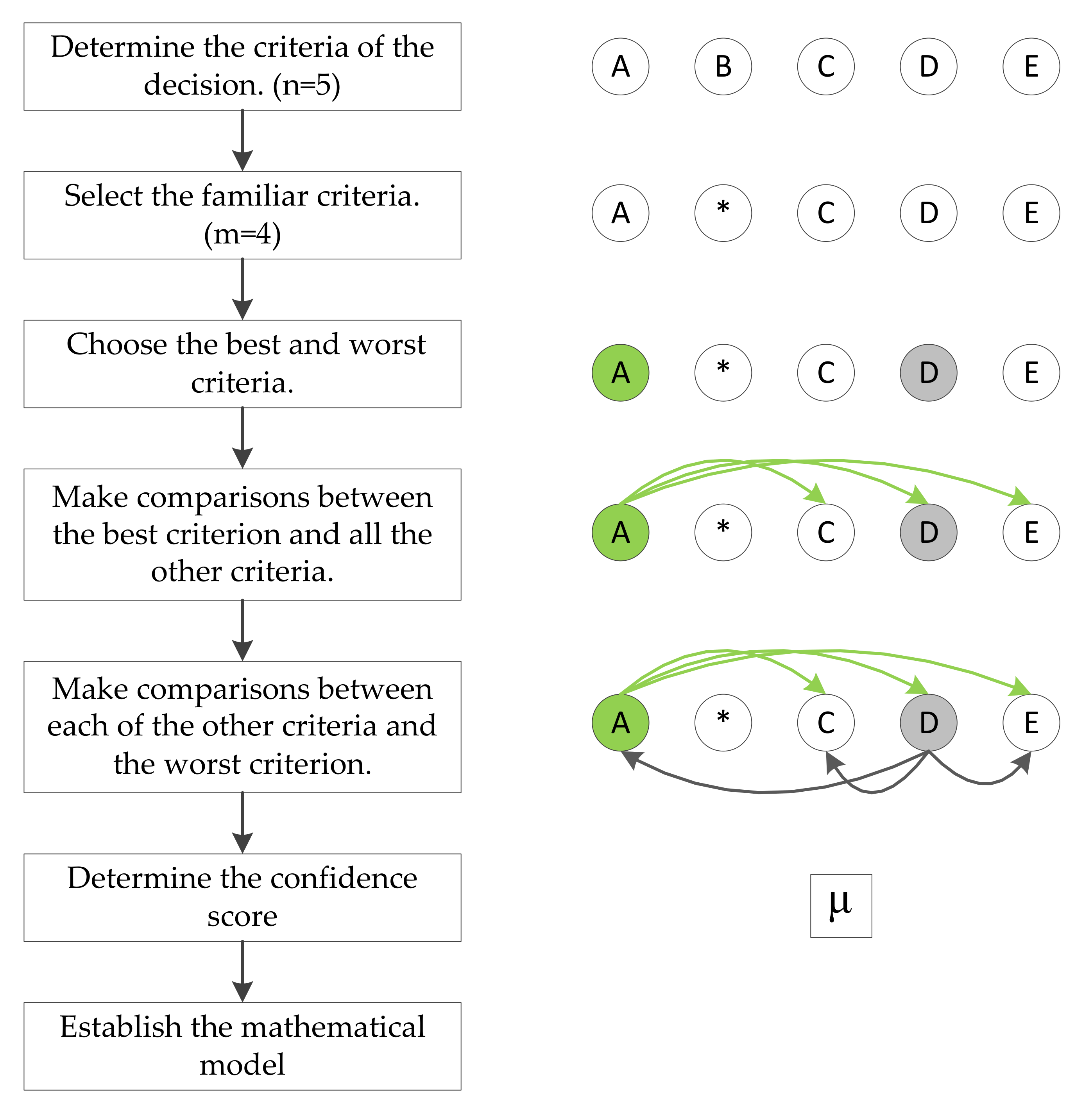


