Hybrid Optimization Based Mathematical Procedure for Dimensional Synthesis of Slider-Crank Linkage

Abstract

In this paper, an optimization procedure for path generation synthesis of the slider-crank mechanism will be presented. The proposed approach is based on a hybrid strategy, mixing local and global optimization techniques. Regarding the local optimization scheme, based on the null gradient condition, a novel methodology to solve the resulting non-linear equations is developed. The solving procedure consists of decoupling two subsystems of equations which can be solved separately and following an iterative process. In relation to the global technique, a multi-start method based on a genetic algorithm is implemented. The fitness function incorporated in the genetic algorithm will take as arguments the set of dimensional parameters of the slider-crank mechanism. Several illustrative examples will prove the validity of the proposed optimization methodology, in some cases achieving an even better result compared to mechanisms with a higher number of dimensional parameters, such as the four-bar mechanism or the Watt’s mechanism.

1. Introduction

Dimensional synthesis consists of finding a geometry that enables a mechanism to generate certain motion characteristics, such as trajectories or positions of elements. It is tough to solve this problem intuitively and often requires the implementation of specific methods. Depending on the type and amount of prescribed motion characteristics, it is not always possible to obtain an exact solution to this problem, forcing us to use optimization methods to find an approximation with minimal error. The target most commonly addressed in bibliographies is the synthesis type, known as path generation, where a point of a single degree of freedom mechanism is sought to run through a sequence of prescribed positions. This motion may or may not be synchronized with the location of the input element, resulting in prescribed or unprescribed timing problems, respectively. It should be noted that there also exist two other goals that are frequently studied, these being beyond the scope of this paper. These are function generation, where the motion of two elements of the mechanism is synchronized, and motion generation, where a sequence of locations for a certain element of the mechanism is prescribed.

Most of the literature on dimensional synthesis focuses on individual cases, the four-bar hinged mechanism being the most widely studied. In the existing literature, both the exact synthesis, by means of graphic [1] or analytical methods [2], and the approximate synthesis, by means of dimensional optimization [3,4], have been studied. On the other hand, the slider-crank mechanism has been used to solve function generation problems [5,6,7,8], for dynamic synthesis [9,10], and to serve as an adjustable mechanism [11,12,13,14]. However, no publications on dimensional optimization for path generation have been found. It should be noted that, in addition to the usual kinematic objectives, some papers include more specific characteristics within the error function. For example, in [15] a formulation is developed by using exact differentiation that allows for establishing the position of the instant center of rotation and the centrode.

An often-employed dimensional optimization procedure consists of minimizing the error function, formulated as the sum of squared differences between the points of the discretized prescribed path, and those belonging to the real generated path. The minimization process can be solved with different methods that can be classified into two main groups, these being local and global methods, which are mentioned below. On the other hand, there are also publications focused not so much on studying the mathematical optimization techniques, but on proposing new ways of describing the output generated by the mechanism. This may result in a more advantageous definition for the optimization error function or for the elaboration of atlases and databases. In relation to the path generation problems discussed in this paper, there exist different approaches to describe the trajectories, and probably the most typical ones are based on the Fourier series [16] or Haar Wavelet transform [17]. Similarly, reference [18] describes a unified theory of the harmonic characteristic parameter method for mechanism synthesis. Apart from the dimensional synthesis, other publications focus on the phase that precedes it, i.e., structural synthesis, the first step in the conceptual design of mechanisms. In this sense, there can be found some proposals of automatic algorithms intended for the structural synthesis of robots and closed-loop mechanisms [19].

In relation to the mathematical optimization techniques for dimensional synthesis, the most effective and widely used local methods consist of applying the null gradient condition, which leads to a non-linear system of equations. This system often includes some passive variables that cannot be eliminated. To solve it, the function is linearized and an iterative method, such as Gauss–Newton, is used, starting from an approximate initial solution provided by the designer. The original reference for this type of method is a paper published in 1966 by Chi-Yeh [20], which was dedicated to the four-bar linkage. From then on, several papers related to dimensional synthesis of this mechanism by means of gradient methods have been published, exploring different ways to improve the effectiveness of optimization. As part of these alternative approaches, in [21] the authors proposed modifying the set of variables to be optimized, considering the nodal coordinates instead of the usual dimensional parameters, thereby allowing the elimination of some constraints that were present in the original problem. It is also noteworthy that other publications focus on reformulating the error function, such as [22,23]. The authors of those works proposed to minimize the strain energy originated when the mechanism is forced to run exactly through the prescribed trajectory. On the other hand, some authors have chosen to estimate the error by avoiding its sensitivity to translation and rotation effects, such as [24], where a system of relative coordinates between precision points is used. Following the same idea, the authors proposed to perform a prior and independent phase to optimize the translation, rotation, and scaling parameters [25]. In addition to the different alternatives to characterize the design parameters of the mechanism and to estimate the resulting error, a relevant aspect to achieve good performance in gradient methods is to carry out an exact calculation of the partial derivatives, avoiding the numerical derivation, since it increases the computational cost and results in a lower efficiency. Given the interest in solving this problem, reference [26] presents a general method for calculating the exact partial derivatives from the loop equations previously identified by the designer.

Despite the large number of existing publications devoted to optimal dimensional synthesis by means of gradient methods, and to the improvement of their performance, none of them are capable of solving the main limitation they have. Unfortunately, these methods are highly sensitive to the chosen starting approximation, since they are local in nature and hence converge to the nearest minimum, which will not necessarily be the optimal overall solution. To overcome this drawback, global methods make it possible to explore the entire space where solutions can be found. Metaheuristic methods are the most common ones, and they have been covered in several references. These include genetic algorithms [27,28,29], differential evolution [30,31,32], ant search [33], krill herd algorithm [34], imperialist competitive algorithm [35], or neural networks [36]. Nevertheless, the weakness of heuristic methods in comparison with gradient methods is their higher computational cost and a lower convergence rate. Furthermore, there is no guarantee that they will converge to a minimum, neither locally nor globally.

Hybrid optimization algorithms, such as [37], gain greater strength when a global method generating seeds for starting mechanisms is combined with a good local method. Normally, hybrid methods start by running a global method to obtain one or several designs that will later be used as initial approximations in a local method to quickly converge to the nearest relative minimum. In this paper, as described below, a hybrid optimization approach is proposed.

In the case of the slider crank mechanism analyzed in this paper, thanks to the simplicity of its kinematics, it is possible to express the synthesis variables directly as a function of the dimensional and input parameters, and thus completely eliminating the passive variables. A novel aspect of the proposed approach is the way in which the resulting system of equations is solved. Considering the more general case of unprescribed timing synthesis, the final system of equations associated with the null gradient condition can be divided into two subsystems with different characteristics. As will be explained, the procedure described in this article allows each subsystem to be solved separately within an iterative process that connects them together. This makes it possible, in some particularly simple cases, such as the two-parameter slider-crank, to solve all the equations analytically, while in more complex cases, numerical methods must necessarily be adopted. The optimum solution reached will be a relative minimum of the error function and will be influenced by the initial approximation used to solve the system of equations numerically. In this paper, reducing this dependency will be attempted by running the local optimization algorithm from different starting points previously selected by a genetic algorithm. The generation of the starting points could also be done by another type of heuristic method, or through a sweeping process that generates random points within the entire search space. Even so, the latter technique would not achieve the most promising regions as the genetic algorithm does, but it would only generate a wide grid of different starting points. Therefore, the genetic algorithm is the preferred choice.

It is important to highlight that the procedure described in this paper seeks to obtain reliable solutions, not only from a mathematical vision, but also from a practical point of view. For this reason, it will be stated how to avoid the circuit defect in the slider-crank mechanism, relying on the concept of branch index. This concept was introduced in reference [21] to analyze the kinematics of the four-bar hinged linkage. The incorporation of design constraints will be addressed by means of penalty functions included in the error function to be minimized. This is essential to impose the Grashof criterion and thus ensure that the input element is able to fully rotate (crank input).

Finally, the effectiveness of the proposed methodology will be illustrated through different examples. The final solutions obtained in this paper are as accurate as the ones reached in other papers when solving the same problem by using more complex designs, such as four-bar or Watt linkages.

The main novelties and highlights of this paper are:

• Deduction of the equations required for the optimal dimensional synthesis of the slider-crank mechanism, which constitutes an alternative to the hinged four-bar linkage usually used in the literature to solve this type of problem.
• Proposal of an original methodology to solve a non-linear system of equations resulting from the null gradient condition, based on the decoupling of two subsystems of equations. It facilitates the resolution of the system and, in some cases, allows to obtain all the solutions in an analytical way.
• Integration of the local optimization methodology within a hybrid optimization method, which uses a genetic algorithm to search for the best starting approximations. The fitness function has been adapted to solve not only the prescribed timing problem, but also unprescribed timing.
• Solving and comparison of examples proposed by other authors in the literature dealing with the four-bar linkage. Thanks to the effectiveness of the method proposed in this work, the slider-crank mechanism, though being simpler and more limited, is able to provide similar performances (or even better in some cases) in path generation problems.

2. Materials and Methods

In this section, the basis of the optimum synthesis procedure as well as the functioning of the hybrid optimization strategy is presented.

2.1. Bases of the Optimum Synthesis Procedure

Before tackling the optimization process, the loop-closure equations of the mechanism and the position equations of the coupler point that traces the trajectory will be obtained. In addition, the variables that take part in the synthesis process and their functional dependence law will be described. This enables obtaining the partial derivatives that intervene in the minimization process.

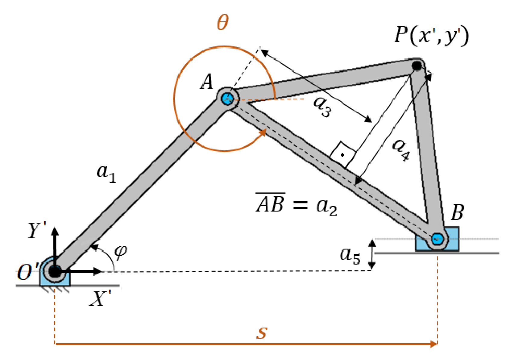
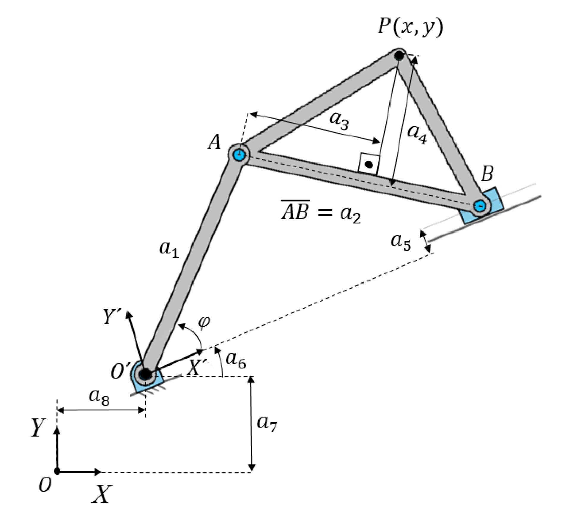
2.1.1. Synthesis Equations for a General Design

First, the kinematic problem of the slider-crank mechanism with five dimensional parameters, represented in Figure 1, is obtained.

The loop-closure equations are the following:

$$a_1·sin\phi =a_5-a_2·sin\theta$$

(1)

$$s=a_1·cos\phi +a_2·cos\theta$$

(2)

From Equation (1) yields:

$$sin\theta =\frac{a_5-a_1·sin\phi }{a_2}$$

(3)

Then, $cos\theta$ is given by Equation (4), where $K=\pm 1$.

$$cos\theta =K\sqrt{1-{\left(\frac{a_5 - a_1·sin\phi }{a_2}\right)}^2}$$

(4)

The synthesis equations are as follows:

$$x^{\prime }=s-\left(a_2-a_3\right)·cos\theta +a_4·cos\left(\theta -\frac{3\pi }{2}\right)$$

(5)

$$y^{\prime }=-(a_2-a_3)·sin\theta +a_5+a_4·cos\theta$$

(6)

Using the loop equations to solve the passive variables $s$ (Equation (2)) and $\theta$ (Equations (3) and (4)), and substituting them in Equations (5) and (6), the following expressions are obtained for the synthesis variables, referring to the local system O’X’Y’:

$$x^{\prime }=a_{1}cos\phi +a_3·K\sqrt{1-{\left(\frac{a_5-a_{1}sin\phi }{a_2}\right)}^2}-\frac{a_4·(a_5-a_{1}sin\phi )}{a_2}$$

(7)

$$y^{\prime }=\frac{ (a_3-a_2)·(a_5-a_{1}sin\phi )}{a_2} cos\phi +a_5+a_4·K\sqrt{1-{\left(\frac{a_5-a_{1}sin\phi }{a_2}\right)}^2}$$

(8)

Remark Regarding Branches and Circuits

The sign $\pm$ in Equations (7) and (8), which has been substituted for $K=\pm 1$ for simplicity, is related to the two possible positions of the coupler point $P$ for the same input $\phi$. This means that two branches exist, each one associated with the positive or negative value of $K$. This circumstance is illustrated in Figure 2, in which the two possible configurations of the mechanism, for a given value of the input $\phi$, are represented.

The two possible trajectories of point $P$ associated with the different configurations of the coupler element, commonly known as branches, can be connected or unconnected, resulting in a unique circuit (a unicursal curve), or two circuits (a bicursal curve). In this work, designs where the crank input is able to perform a 360° full rotation are considered, meaning that the Grashof criterion must be fulfilled. Therefore, the two possible branches will be two unconnected circuits. To avoid branch defects, all the selected points must have the same value of $K$. This value will be the one corresponding to the branch that yields a minimum error with respect to the desired path.

In the most general case, represented in Figure 3, the local reference system O’X’Y’ has a rotation relative to the global system OXY, defined by the parameter $a_6$, and a translation in the plane defined by the parameters $a_7$ and $a_8$.

The equations that express the synthesis variables in the global reference system are the following:

$$x_i=x_i{}^{\prime }·cos\left(a_6\right)-y_i{}^{\prime }·sin\left(a_6\right)+a_8$$

(9)

$$y_i=x_i{}^{\prime }·sin\left(a_6\right)+y_i{}^{\prime }·cos\left(a_6\right)+a_7$$

(10)

Now that all the variables involved in the synthesis problem have been defined, the following classification can be established:

• Dimensional variables: $a_1,a_2,\dots ,a_8$. These are variables that define the lengths of the bars and the translation or rotation parameters of the studied mechanism.
• Input variable: $\phi$. This is an independent variable corresponding to the degree of freedom of the mechanism under study.
• Passive variables: $\theta ,s$. These are not independent variables, but rather depend on the input and the dimensional parameters.
• Output variables or synthesis variables: $x, y$. These correspond to the coordinates of the coupler point P. In the case of path generation synthesis, these are indeed the synthesis variables.

2.1.2. Optimal Design Based on the Error Function

The error function $E$, commonly used in synthesis problems, is defined as the sum of the squared Cartesian distances between the prescribed points and those actually generated:

$$E={\displaystyle \sum }_{i=1}^N \left[{\left(x_i-x_i^d\right)}^2+{\left(y_i-y_i^d\right)}^2\right]$$

(11)

The error between prescribed and generated trajectory must be minimized to obtain the optimal mechanism. There are two options for carrying out this minimization. In the modality known as prescribed timing, only the dimensional parameters are optimized, requiring solving the system shown in Equation (12). In this case, the input parameters ${\phi }_i$ are not variables to be optimized, but constant values (prescribed values). However, in an optimization known as unprescribed timing, both the dimensional parameters $a_j$ and the set of input parameters ${\phi }_i$ are optimized, requiring solving the systems given by Equations (12) and (13). This last option is more complex but its potential to obtain precise solutions is greater, since the value of the input parameters is not being restricted.

$$\frac{\partial E}{\partial a_j}=0 \to {\displaystyle \sum }_{i=1}^N\left[\left(x_i-x_i^d\right)\frac{\partial x_i}{\partial a_j}+\left(y_i-y_i^d\right)\frac{\partial y_i}{\partial a_j}\right]=0 \forall j=1,2,\dots ,n$$

(12)

$$\frac{\partial E}{\partial {\phi }_i }=0 \to {\displaystyle \sum }_{i=1}^N\left[\left(x_i-x_i^d\right)\frac{\partial x_i}{\partial {\phi }_i }+\left(y_i-y_i^d\right)\frac{\partial y_i}{\partial {\phi }_i }\right]=0 \forall i=1,2,\dots ,N$$

(13)

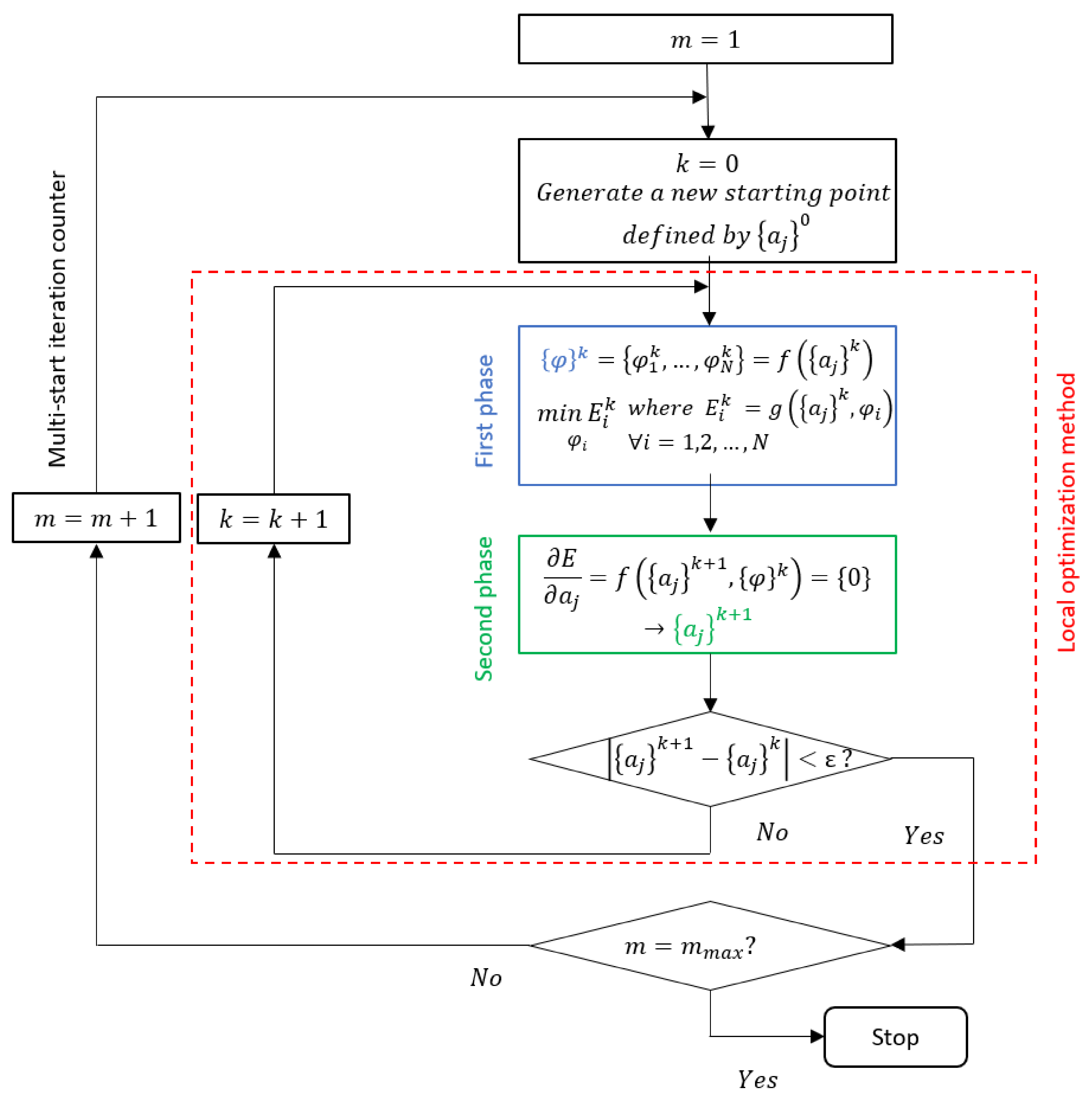
2.2. Hybrid Optimization Procedure

Thanks to the simplicity of its kinematics, in the slider-crank mechanism it is possible to eliminate the passive variables. In this way, the synthesis variables $\left(x,y\right)$ are expressed as an explicit function of parameters $\left\{a_j\right\}$ and $\phi$, facilitating the obtaining of the partial derivatives that appear in Equations (12) and (13). After performing the substitution, it can be verified that the system of Equations (12) and (13) is non-linear. This system can be decomposed into two subsystems of equations. On the one hand, Equation (12) is composed of 8 equations, as many as the dimensional parameters of the mechanism. Each of these equations has the form $g\left(a_1,a_2\dots a_8,{\phi }_1,{\phi }_2,\dots {\phi }_N\right)=0$. On the other hand, Equation (13) is made up of N equations, as many as points of precision has the trajectory. Each of these equations has the form $h\left(a_1,a_2\dots a_8,{\phi }_i\right)=0$. This circumstance is fundamental when establishing the procedure for solving the system of equations.

In addition, in order to find the optimal initial approximation, the one that will be the starting point of the local optimization process, and that plays a relevant role in the process, a multi-start approach will be implemented. In the following sections, the hybrid procedure proposed by the authors of this work will be explained.

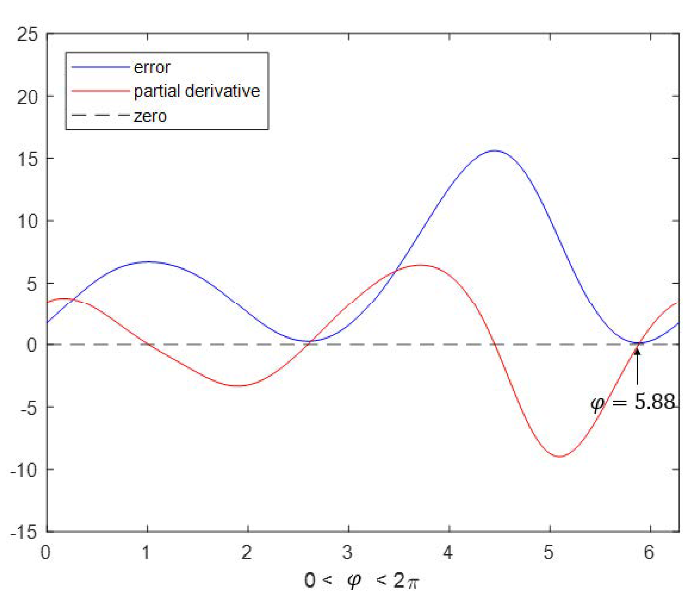
2.2.1. Solving the Equation System for Local Optimization

In this section, the iterative algorithm to solve the non-linear system of equations resulting from the null gradient condition is addressed. The procedure is based on the decoupling of the two subsystems (12) and (13), as described below.

• First phase:

This starts from a certain mechanism, coming from the multi-start procedure that will be explained in Section 3.2. The dimensions ($a_1,a_2,\dots ,a_8$) of this mechanism are assumed constant in this phase. The values of these dimensions are substituted in each of the equations of subsystem (13), resulting in a total of N equations, each with a unique ${\phi }_i$.

In the simplest case of the slider-crank mechanism, with 2 dimensional parameters ($a_1=a_2=a_3$ and $a_5=a_6=a_7=a_8=0$), and using the transformation of half-angle tangent, $t_i=\tan \frac{{\phi }_i}{2}$, Equation (13) becomes a fourth degree polynomial:

$$\left(2a_1{a}_4+x_i^d{a}_4\right)t_i^4+\left(8a_1{}^2+x_i^d{a}_1+2y_i^d{a}_4\right)t_i^3-12a_1{a}_4{t}_i^2+\left(-8a_1{}^2+4x_i^d{a}_1+2y_i^d{a}_4\right)t_i+2a_1{a}_4-x_i^d{a}_4=0$$

(14)

From the 4 possible values of $t_i\left({\phi }_i\right)$, the one that gives the minimum error is the selected one.

For a design with 3 dimensional parameters, Equation (13) becomes a polynomial of degree 10. Even so, it is easy to obtain the 10 roots and detect the correct one proceeding as in the previous case. However, with 4 or more dimensional parameters, it is no longer as easy to determine its corresponding univariate polynomial, nor is it really worth it. It is more practical to operate as explained next.

The Equation (13) is solved numerically, starting from an initial approximation, and arriving at a unique solution of the parameter ${\phi }_i$. To guarantee that the global optimal value of ${\phi }_i$ is obtained, it will be necessary to start from an initial approximation obtained as follows: each sum of Equation (11), which represents the error made in each synthesis position $i$, is evaluated as a function of the input parameter ${\phi }_i$ along the discretized domain [0,2π). In this way, a graph similar to the blue curve represented in Figure 4 will be obtained, where two minima of the error function appear, the one indicated on the right being the one with the lowest value. The latter value of ${\phi }_i$ is taken as a starting approximation to solve Equation (13) (in our case, using the MATLAB fsolve command).

To illustrate this concept, in Figure 5 the prescribed point for a synthesis position $i$ and the trajectory generated by the mechanism of dimensions $\left\{a_j\right\}$ in the current iteration are indicated. The effect of evaluating the sum of the error function (11) and choosing the absolute minimum is equivalent to traversing the generated trajectory and selecting the point of it (the black point) closest to the prescribed one (red point). In this example, the black point indicated in Figure 5 corresponds to the absolute minimum, $\phi =5.88$ rad, which is the one previously indicated in Figure 4.

• Second phase:

In this phase, the values ${\phi }_i$ obtained in the previous phase will be assumed as constants, and the unknowns ($a_1,a_2,\dots ,a_8$) will be calculated from the subsystem from Equation (12).

As an example, in the simplified particular case of the slider-crank mechanism with 2 parameters, Equation (12) becomes the following linear system:

$$\left[\begin{array}{cc}4{\displaystyle \sum _{i=1}^N}co{s}^2{\phi }_i& {\displaystyle \sum _{i=1}^N}sin2{\phi }_i\\ {\displaystyle \sum _{i=1}^N}sin2{\phi }_i& N\end{array}\right]\left\{\begin{array}{c}{a}_1\\ \\ \\ \\ a_4\end{array}\right\}=\left\{\begin{array}{c}2{\displaystyle \sum _{i=1}^N}cos{\phi }_i\cdot x_i^d\\ {\displaystyle \sum _{i=1}^N}\left(sin{\phi }_i\cdot x_i^d+cos{\phi }_i\cdot y_i^d\right)\end{array}\right\}$$

(15)

However, in the design cases with 3 or more dimensional parameters, the subsystem of equations turns out to be non-linear, making it necessary to apply numerical solving methods. As a starting approximation, the values ($a_1,a_2,\dots ,a_8$) that were assumed as constants in the previous phase will be taken.

• Next steps:

With the new values of $\left\{a_j\right\}$ obtained in the second phase, we go back to the first phase, and thus continue iteratively until convergence. The chosen stopping criterion consists of comparing the current values of the optimization variables $\left(a_1,a_2\dots a_8,{\phi }_1,{\phi }_2,\dots {\phi }_N\right)$ with those of the previous iteration, so that when the difference is less than a specified tolerance, the iterative process will stop.

2.2.2. Implementing a Multi-Start Strategy

The method proposed in Section 3.1 has the disadvantage of being very sensitive to the starting approximation. To avoid this drawback, a multi-start approach based on a genetic algorithm will be used to guide the local optimization method towards a search for the global optimal solution.

The proposed multi-start approach obtains a sufficiently large set of starting approximations, representative of a global sweep of the design space $\left\{a_j\right\}$. In this article, a genetic algorithm is used to locate 100 candidate solutions that serve as initial approximations. It is decided to use the genetic algorithm incorporated in MATLAB, assigning as arguments of the fitness function the values for the 8 dimensional parameters. The latter function assigns the optimal correspondence of input parameters, according to the procedure outlined in the first phase of Section 3.1, and returns a scalar value that quantifies the individual’s fitness as the quadratic sum of the distances between generated and prescribed points.

It is important to bear in mind that, considering the way the fitness function is posed, each starting solution for the unprescribed timing problem will not depend on $8+N$ variables (8 dimensional + $N$ inputs), but only on the 8 dimensional parameters, which facilitates the exploration of the search space by the genetic algorithm without the need to restrict the input parameters.

The complete scheme of this hybrid procedure is shown in Figure 6. As can be seen, it consists of executing a local optimization from the different starting points obtained in the scan of the space of the dimensional parameters $\left\{a_j\right\}$. In this way, different local minimums will be obtained and the best of them will be selected.

To avoid excessive computational cost, the execution time of the genetic algorithm is limited to an acceptable value (i.e., 1 min). Bear in mind that it will not be necessary to obtain the optimal solutions, but that it will be enough to be close to them. On the other hand, the execution time of the local method to be applied later will depend on the number of iterations performed, but it generally consumes a few seconds for each starting point used.

2.2.3. Incorporation of Design Constraints

Searching for an optimal design usually implies adapting the generated trajectory to a prescribed one. In addition, some design requirements must be fulfilled. These design constraints are related to several aspects, such as the maximum size of the mechanism, the maximum and minimum lengths of certain bars, the Grashof criterion, the transmission angle limits, and so on.

In general, the optimization problem with certain inequality constraints can be formulated as the minimum error subjected to

$$g_k\left\{a_1,\dots ,a_n\right\}\ge 0 \forall k=1,2,\dots ,l$$

A typical constraint equation, $g_k$, is expressed as follows:

$${\displaystyle \sum }_{j=1}^m{a}_j{C}_j\ge C_0$$

(16)

When an inequality constraint, such as Equation (16), is included in the process, the error function yields

$$E={\displaystyle \sum }_{i=1}^N{\left(x_i-x_i^d\right)}^2+{\displaystyle \sum }_{i=1}^N{\left(y_i-y_i^d\right)}^2+\lambda ·{\left({\displaystyle \sum }_{j=1}^m{a}_j{C}_j-C_0\right)}^2$$

(17)

If, on the one hand, Equation (16) is not fulfilled during the iterations of the optimization process, it is necessary to amplify the value of the error to invalidate the corresponding design $\left\{a_j\right\}$. This can be done by means of the $\lambda$ parameter, which acts as a penalty factor, proceeding as follows:

$$\begin{array}{c}\mathrm{If} {\displaystyle \sum _{j=1}^m}{a}_j{C}_j-C_0<0 \mathrm{then} \lambda =Predefined value \\ \mathrm{If} {\displaystyle \sum _{j=1}^m}{a}_j{C}_j-C_0\ge 0 \mathrm{then} \lambda =0 \end{array}$$

If, on the other hand, the condition to be imposed is an equality constraint, then $\lambda$ will always be a certain predefined value. In this paper, after reviewing similar works in the literature and conducting several trials with different values, the value $\lambda =50$ was established, insofar as it provides good results for all the analyzed design cases.

3. Results

The following examples will demonstrate the validity of the proposed methodology, showing the results of each design case.

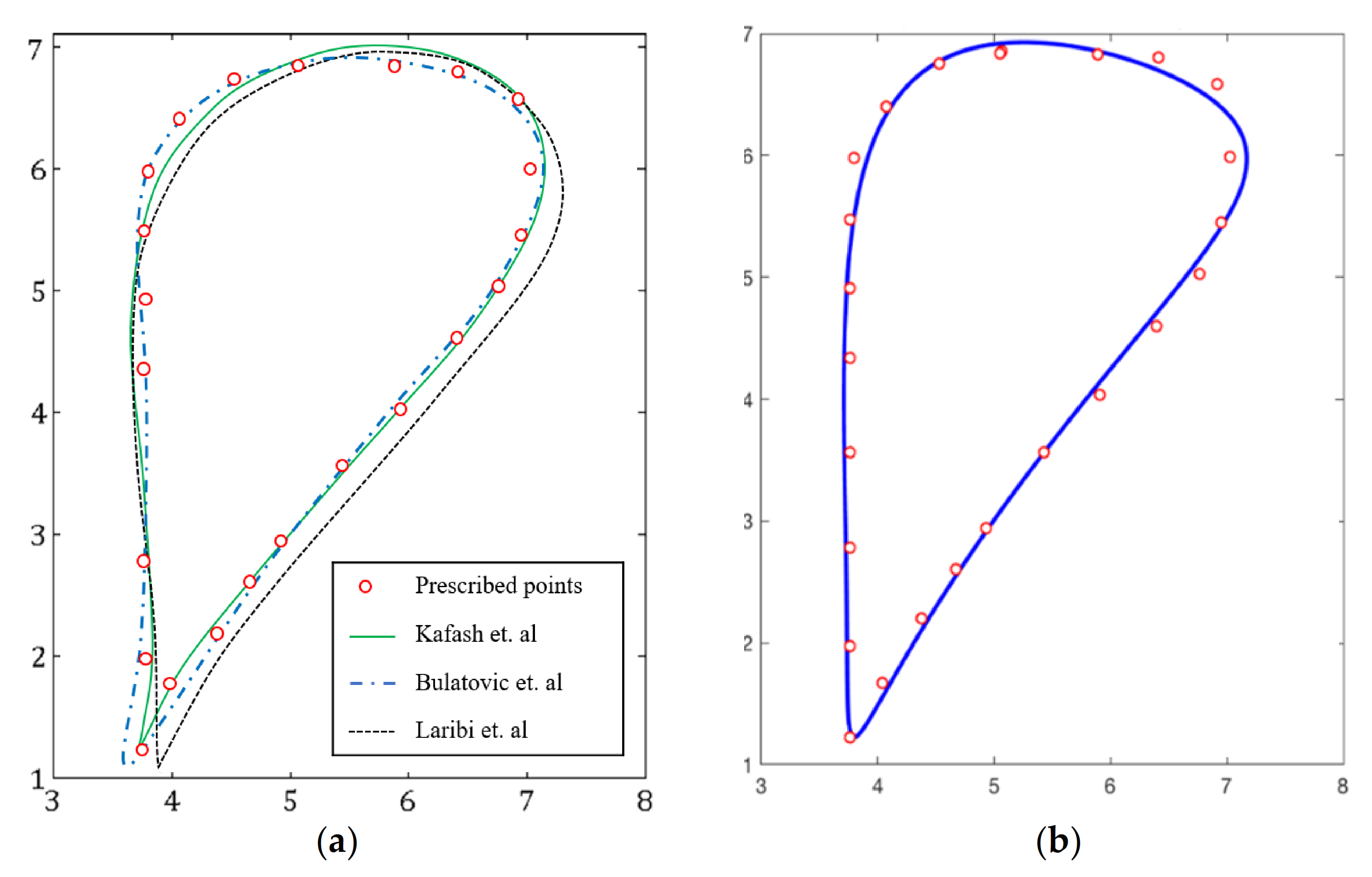
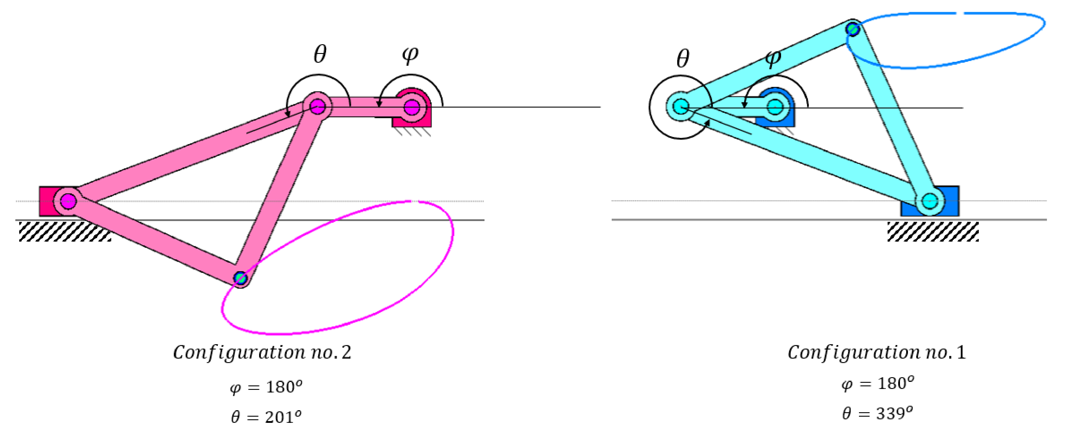
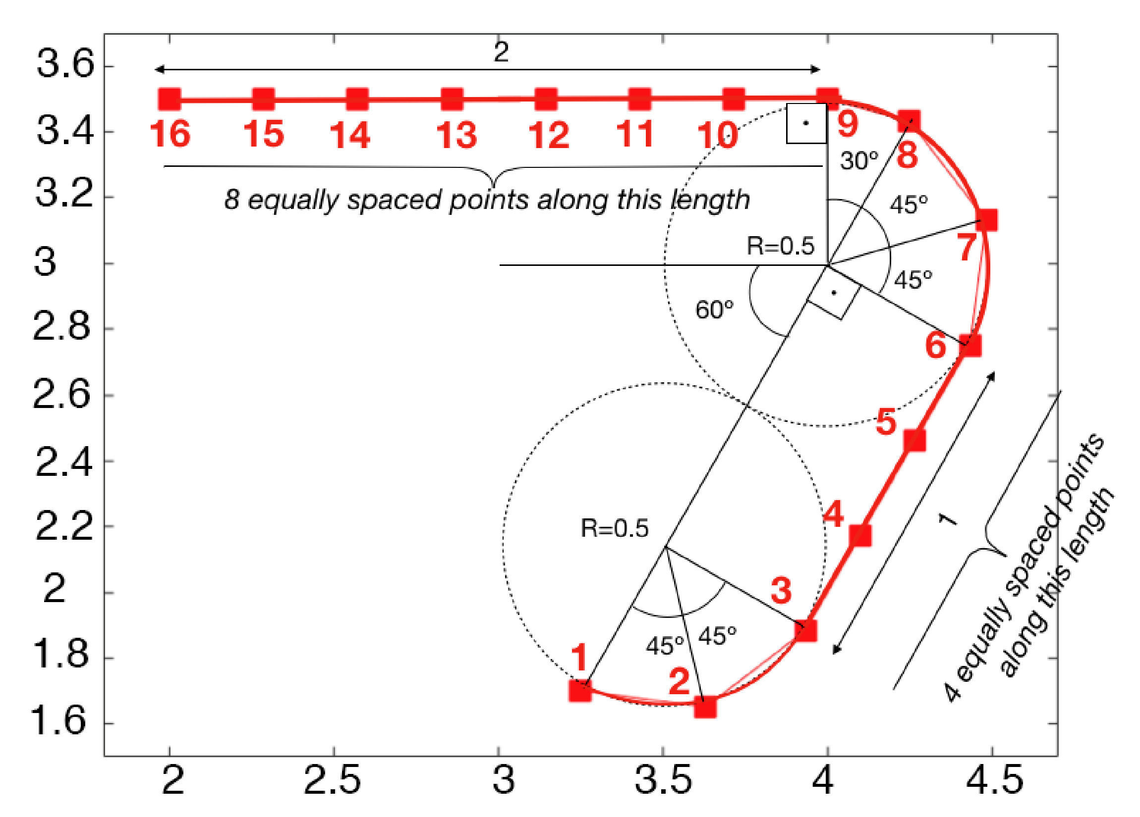
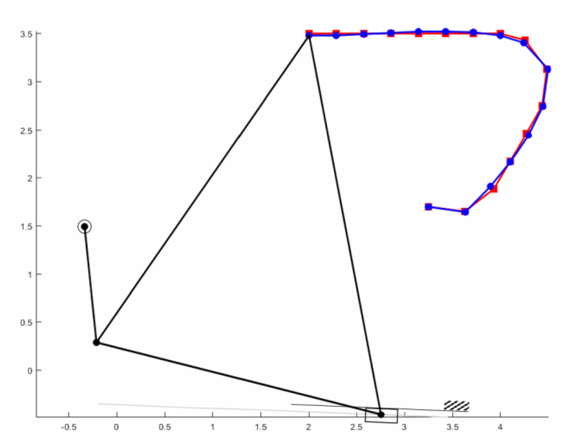
3.1. Demonstrative Example 1

The desired trajectory, shown in Figure 7, is formed by two straight lines and two circumference arcs tangent to these lines. Considering the simplicity of the slider-crank, achieving a design that traces this trajectory is challenging. Moreover, this example is interesting because the trajectory combines both straight lines and arcs, which are trajectories commonly used in the path planning synthesis of planar mechanisms. The coordinates of the desired points, $\left(x_i^d,y_i^d\right)$, are given in

Table 1. Example 1. Initial data.

i	${\mathit{x}}_{\mathit{i}}^{\mathit{d}}$	${\mathit{y}}_{\mathit{i}}^{\mathit{d}}$
1	3.2500	1.7010
2	3.6294	1.6510
3	3.9330	1.8840
4	4.0995	2.1724
5	4.2665	2.4616
6	4.4330	2.7500
7	4.4829	3.1294
8	4.2500	3.4330
9	4.0000	3.5000
10	3.7143	3.5000
11	3.4286	3.5000
12	3.1429	3.5000
13	2.8571	3.5000
14	2.5714	3.5000
15	2.2857	3.5000
16	2.0000	3.5000

. A total of 16 points are defined.

The eight dimensional parameters and the 16 input parameters (unprescribed timing) will be optimized, that is, the most complete case possible. Following the previously described technique, this example is solved using the proposed multi-start method, starting from 100 different starting mechanisms. The conditions of the crank-input (based on Grashof’s criterion) and a maximum 3:1 ratio between the longest and shortest bar are imposed by means of penalty functions.

The best solution, shown in Figure 8, leads to an error equal to 0.0073. The corresponding design parameters are included in

Table 2. Example 1: optimum design parameters and inputs.

Parameters		Inputs
a1	1.292	φ1	4.877	φ9	2.992
a2	3.277	φ2	4.568	φ10	2.804
a3	1.292	φ3	4.409	φ11	2.634
a4	3.875	φ4	4.267	φ12	2.476
a5	1.970	φ5	4.104	φ13	2.323
a6	3.090	φ6	3.905	φ14	2.171
a7	1.356	φ7	3.579	φ15	2.014
a8	−0.583	φ8	3.192	φ16	1.846

. In the Supplementary Materials, a video showing the motion of this optimum mechanism can be found.

To illustrate the influence that the starting point has on the final solution obtained, Figure 9 shows, by way of example, the optimal mechanism obtained from another starting point, which does not reach a solution as good as the one shown above, so it would be excluded.

This same example has been used by the authors of this work in a recent work, in particular reference [38], making use of another optimization method and applying it to the four-bar mechanism. It should be taken into account that the four-bar mechanism has an additional dimensional parameter with respect to the slider-crank and thus, in principle, a greater potential to adjust to the prescribed trajectories. Nevertheless, comparing the results of both achieved optimal mechanisms (the error in [38] with the four-bar was 0.0089), it can be seen that they are almost of the same value, even having a slightly smaller error in the current case.

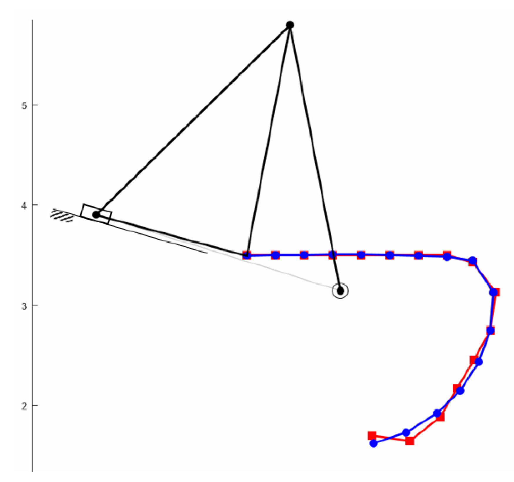
3.2. Demonstrative Example 2

Figure 10a shows the results obtained by other authors [30,34,39,40] for an example of path generation synthesis of a closed path formed by 25 points marked in red. Each of the authors uses a different optimization method, but all of them use the four-bar mechanism. On the other hand, Figure 10b shows the results obtained when solving the same example with the slider-crank under the methodology proposed in this paper.

The comparison is made with other studies that analyze the four-bar because, as mentioned in the introduction, the vast majority of path generation synthesis works make use of the four-bar. Even so, as it has been shown in the previous example and it will happen in this one, the method that we propose achieves very similar (or even better) results, despite making use of a more limited mechanism such as the slider-crank.

The optimal solution obtained in this paper with the slider-crank mechanism (Figure 10b) corresponds to an error of 0.103 and is of similar quality to Bulatović et al. [34]. They obtained an error of 0.0392, which is slightly lower than the one we found, but is of the same order of magnitude. On the other hand, in [34] they also indicated the error achieved by Laribi et al. [39] and Smaili and Diab [40], these being 0.9022 and 0.5504, respectively, so they would be considerably higher. On the other hand, the error obtained by Kafash and Nahvi [30] is not directly comparable with the rest because they use a different error function. However, the trajectory generated by the authors in [30] is graphically represented in Figure 10a.

The corresponding optimal design parameters for the more general case of slider-crank are shown in

Table 3. Example 2: Optimum design parameters and inputs.

Parameters		Inputs
a1	2.309	φ1	4.703	φ9	−0.237	φ17	2.715	φ25	4.451
a2	48.819	φ2	4.92	φ10	0.049	φ18	2.933
a3	−3.304	φ3	5.041	φ11	0.672	φ19	3.17
a4	24.498	φ4	5.181	φ12	1.331	φ20	3.483
a5	46.315	φ5	5.362	φ13	1.698	φ21	3.762
a6	4.726	φ6	5.528	φ14	1.996	φ22	3.752
a7	−18.02	φ7	5.745	φ15	2.281	φ23	4.091
a8	15.293	φ8	5.875	φ16	2.494	φ24	4.265

. As in the previous example, a video showing the motion of this optimum mechanism is included as Supplementary Materials.

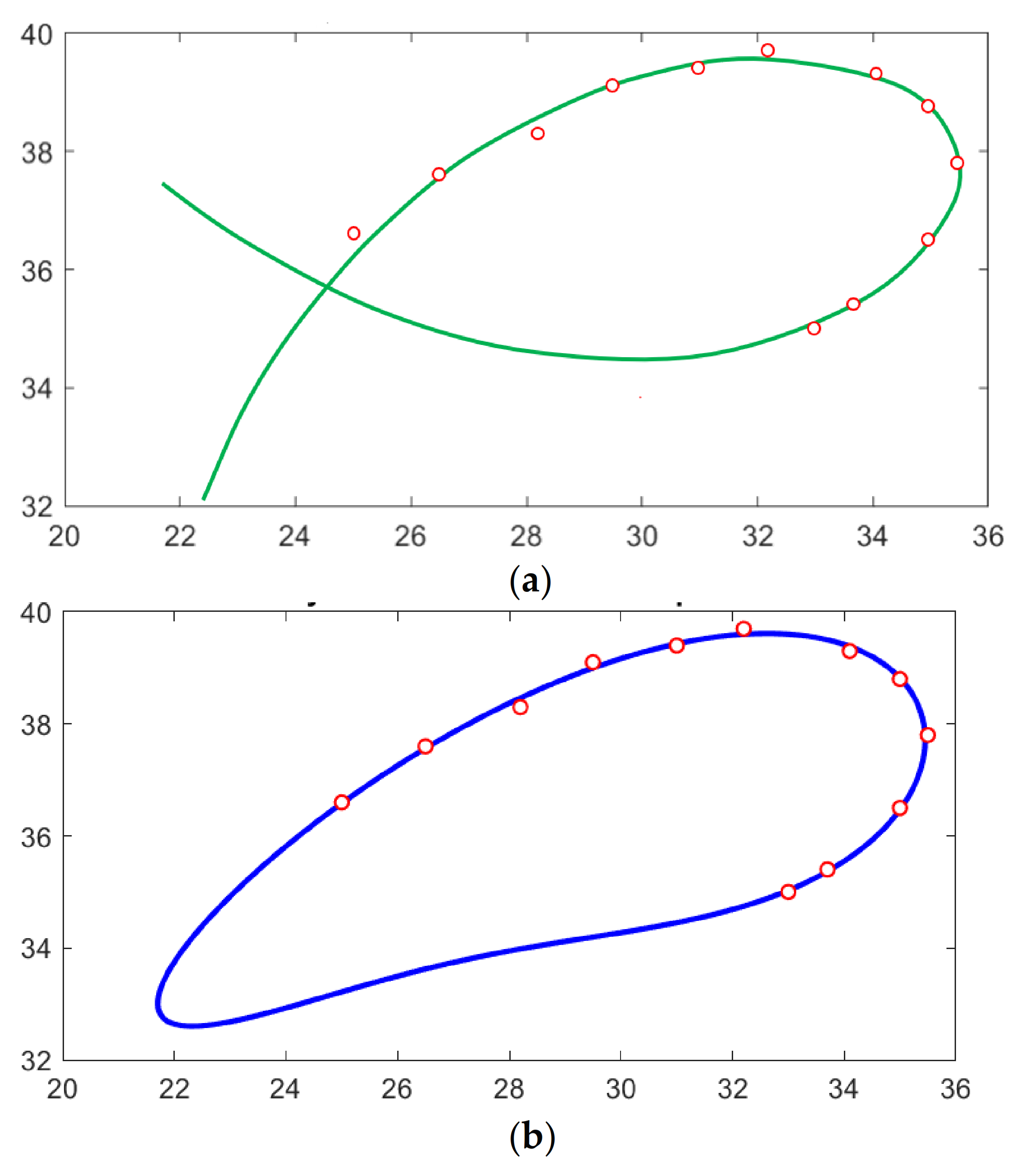
3.3. Demonstrative Example 3

On this occasion, a path generation problem, previously solved in reference [41] for the Watt mechanism, is presented. Their optimal solution is represented in Figure 11a, together with the set of prescribed points represented in red. The optimal solution obtained with the slider-crank mechanism, represented in Figure 11b, has an equal, and, it could be said, even higher precision, despite being a simpler mechanism that has fewer design parameters involved.

The optimal design parameters of the slider-crank mechanism are listed in

Table 4. Example 3: Optimum design parameters and inputs.

Parameters		Inputs
a1	6.719	φ1	5.580	φ9	3.502
a2	15.635	φ2	5.349	φ10	3.101
a3	5.217	φ3	5.116	φ11	2.708
a4	8.737	φ4	4.918	φ12	2.549
a5	−6.710	φ5	4.703
a6	−2.924	φ6	4.508
a7	42.513	φ7	4.124
a8	35.584	φ8	3.848

. Yet again, a video showing the motion of this optimum mechanism is included as Supplementary Materials.

4. Discussion

In this paper, a hybrid optimization procedure has been presented to address the dimensional synthesis of path generation using the slider-crank mechanism. On the one hand, a novel approach has been proposed to solve the non-linear equations corresponding to the null gradient condition, which is based on the decoupling of two subsystems of equations, and which simplifies the resolution procedure without prejudice to the precision obtained. On the other hand, the incorporation of the multi-start method manages to give the local optimization method a global character, carrying out a previous sweep of the total space of the dimensional variables to find the most promising starting approximations. To carry out this search, a genetic algorithm is used where only the eight dimensional parameters are involved, thanks to the fact that the fitness function has been programmed to select the optimal input parameters based on the dimensions.

In addition, it should be noted that this methodology is aimed at achieving designs that are valid from a practical point of view. Therefore, the non-existence of branch defects is ensured, and different design restrictions can be incorporated in a simple way through the use of penalty functions. In this way, it can be ensured that the crank input mechanism does not exceed a maximum ratio between bar lengths or other additional design requirements at the discretion of the designer.

Finally, the effectiveness of the method has been proved by verifying, through various examples, that the slider-crank mechanism allows us to achieve solutions with a precision comparable to other one degree of freedom mechanisms that have a greater number of dimensional parameters, such as the four-bar or the Watt’s mechanism, with the additional advantage of having simpler kinematics.

References

1. Erdman, A.G.; Sandor, G.N. Mechanism Design: Analysis and Synthesis, 4th ed.; Pearson: London, UK, 2001. [Google Scholar]
2. Wampler, C.; Morgan, A.P.; Sommese, A.J. Complete Solution of the Nine-Point Path Synthesis Problem for Four-Bar Linkages. J. Mech. Des. 1992, 114, 153–159. [Google Scholar] [CrossRef]
3. Lee, W.-T.; Russell, K. Developments in quantitative dimensional synthesis (1970-present): Four-bar motion generation. Inverse Probl. Sci. Eng. 2017, 26, 133–148. [Google Scholar] [CrossRef]
4. Lee, W.-T.; Russell, K. Developments in quantitative dimensional synthesis (1970–present): Four-bar path and function generation. Inverse Probl. Sci. Eng. 2018, 26, 1280–1304. [Google Scholar] [CrossRef]
5. Alizade, R.I.; Mohan Rao, A.V.; Sandor, G.N. Optimum Synthesis of Four-Bar and Offset Slider-Crank Planar and Spatial Mechanisms Using the Penalty Function Approach with Inequality and Equality Constraints. J. Eng. Ind. 1975, 97, 785–790. [Google Scholar] [CrossRef]
6. Rao, A.C. Optimum synthesis of a slider-crank mechanism using geometric programming. Int. J. Numer. Methods Eng. 1980, 15, 1595–1602. [Google Scholar] [CrossRef]
7. Plecnik, M.M.; McCarthy, J.M. Five position synthesis of a slider-crank function generator. In Proceedings of the ASME International Conference IDETC/CIE 2011, Washington, DC, USA, 28–31 August 2011; pp. 317–324. [Google Scholar]
8. Almandeel, A.; Murray, A.P.; Myszka, D.H.; Stumph, H.E. A Function Generation Synthesis Methodology for All Defect-Free Slider-Crank Solutions for Four Precision Points. J. Mech. Robot. 2015, 7, 031020–031021. [Google Scholar] [CrossRef]
9. Liniecki, A. Synthesis of a slider-crank mechanism with consideration of dynamic effects. J. Mech. 1970, 5, 337–349. [Google Scholar] [CrossRef]
10. Davidson, J.K. Analysis and synthesis of a slider-crank mechanism with a flexibly-attached slider. J. Mech. 1970, 5, 239–247. [Google Scholar] [CrossRef]
11. Zhou, H.; Ting, K.-L. Adjustable slider–crank linkages for multiple path generation. Mech. Mach. Theory 2002, 37, 499–509. [Google Scholar] [CrossRef]
12. Russell, K.; Sodhi, R. On the Design of Slider-Crank Mechanisms. Part I: Multi-Phase Motion Generation. Mech. Mach. Theory 2005, 40, 285–299. [Google Scholar] [CrossRef]
13. Russell, K.; Sodhi, R.S. On the design of slider-crank mechanisms. Part II: Multi-phase path and function generation. Mech. Mach. Theory 2005, 40, 301–317. [Google Scholar] [CrossRef]
14. Zhou, H. Dimensional synthesis of adjustable path generation linkages using the optimal slider adjustment. Mech. Mach. Theory 2009, 44, 1866–1876. [Google Scholar] [CrossRef]
15. Sancibrian, R.; Sarabia, E.G.; Sedano, A.; Blanco, J.M. A general method for the optimal synthesis of mechanisms using prescribed instant center positions. Appl. Math. Model. 2016, 40, 2206–2222. [Google Scholar] [CrossRef]
16. Sun, J.; Chu, J. Fourier series representation of the coupler curves of spatial linkages. Appl. Math. Model. 2010, 34, 1396–1403. [Google Scholar] [CrossRef]
17. Liu, W.; Sun, J.; Zhang, B.; Chu, J. Wavelet feature parameters representations of open planar curves. Appl. Math. Model. 2018, 57, 614–624. [Google Scholar] [CrossRef]
18. Jianwei, S.; Jinkui, C.; Baoyu, S. A unified model of harmonic characteristic parameter method for dimensional synthesis of linkage mechanism. Appl. Math. Model. 2012, 36, 6001–6010. [Google Scholar] [CrossRef]
19. Ding, H.; Huang, P.; Zi, B.; Kecskeméthy, A. Automatic synthesis of kinematic structures of mechanisms and robots especially for those with complex structures. Appl. Math. Model. 2012, 36, 6122–6131. [Google Scholar] [CrossRef]
20. Chi-Yeh, H. A general method for the optimum design of mechanisms. J. Mech. 1967, 1, 301–313. [Google Scholar] [CrossRef]
21. Angeles, J.; Alivizatos, A.; Akhras, A. An unconstrained nonlinear least-square method of optimization of RRRR planar path generators. Mech. Mach. Theory 1988, 23, 343–353. [Google Scholar] [CrossRef]
22. Avilés, R.; Navalpotro, S.; Amezua, E.; Hernández, A. An Energy-Based General Method for the Optimum Synthesis of Mecha-nisms. J. Mech. Des. 1994, 116, 127–136. [Google Scholar] [CrossRef]
23. Vallejo, J.; Avilés, R.; Hernández, A.; Amezua, E. Nonlinear optimization of planar linkages for kinematic syntheses. Mech. Mach. Theory 1995, 30, 501–518. [Google Scholar] [CrossRef]
24. Sancibrian, R.; Viadero, F.; García, P.; Fernández, A. Gradient-based optimization of path synthesis problems in planar mechanisms. Mech. Mach. Theory 2004, 39, 839–856. [Google Scholar] [CrossRef]
25. Sancibrian, R.; De Juan, A.; Sedano, A.; Iglesias, M.; García, P.; Viadero, F.; Fernandez, A. Optimal Dimensional Synthesis of Linkages Using Exact Jacobian Determination in the SQP Algorithm. Mech. Based Des. Struct. Mach. 2012, 40, 469–486. [Google Scholar] [CrossRef]
26. Mariappan, J.; Krishnamurty, S. A generalized exact gradient method for mechanism synthesis. Mech. Mach. Theory 1996, 31, 413–421. [Google Scholar] [CrossRef]
27. Cabrera, J.; Simon, A.; Prado, M. Optimal synthesis of mechanisms with genetic algorithms. Mech. Mach. Theory 2002, 37, 1165–1177. [Google Scholar] [CrossRef] [Green Version]
28. Acharyya, S.; Mandal, M. Performance of EAs for four-bar linkage synthesis. Mech. Mach. Theory 2009, 44, 1784–1794. [Google Scholar] [CrossRef]
29. Buśkiewicz, J.; Starosta, R.; Walczak, T. On the application of the curve curvature in path synthesis. Mech. Mach. Theory 2009, 44, 1223–1239. [Google Scholar] [CrossRef]
30. Kafash, S.H.; Nahvi, A. Optimal synthesis of four-bar path generator linkages using Circular Proximity Function. Mech. Mach. Theory 2017, 115, 18–34. [Google Scholar] [CrossRef]
31. Gogate, G.R.; Matekar, S.B. Optimum synthesis of motion generating four-bar mechanisms using alternate error functions. Mech. Mach. Theory 2012, 54, 41–61. [Google Scholar] [CrossRef]
32. Bulatović, R.R.; Ðorđević, S.R. Control of the optimum synthesis process of a four-bar linkage whose point on the working member generates the given path. Appl. Math. Comput. 2011, 217, 9765–9778. [Google Scholar] [CrossRef]
33. Xiao, R.; Tao, Z. A Swarm Intelligence Approach to Path Synthesis of Mechanism. In Proceedings of the Ninth International Conference on Computer Aided Design and Computer Graphics (CAD-CG’05), Hong Kong, China, 7–10 December 2005; Institute of Electrical and Electronics Engineers (IEEE): Piscataway, NJ, USA, 2005; pp. 451–456. [Google Scholar]
34. Bulatovic, R.R.; Miodragovic, G.; Boskovic, M.S. Modified Krill Herd (MKH) algorithm and its application in dimensional syn-thesis of a four-bar linkage. Mech. Mach. Theory 2016, 95, 1–21. [Google Scholar] [CrossRef]
35. Ebrahimi, S.; Payvandy, P. Efficient constrained synthesis of path generating four-bar mechanisms based on the heuristic opti-mization algorithms. Mech. Mach. Theory 2015, 85, 189–204. [Google Scholar] [CrossRef]
36. Vasiliu, A.; Yannou, B. Dimensional synthesis of planar mechanisms using neural networks: Application to path generator linkages. Mech. Mach. Theory 2001, 36, 299–310. [Google Scholar] [CrossRef] [Green Version]
37. Sedano, A.; Sancibrian, R.; De-Juan, A.; Viadero, F.; Egaña, F. Hybrid Optimization Approach for the Design of Mechanisms Using a New Error Estimator. Math. Probl. Eng. 2012, 2012, 1–20. [Google Scholar] [CrossRef]
38. Hernández, A.; Muñoyerro, A.; Urízar, M.; Amezua, E. Comprehensive approach for the dimensional synthesis of a four-bar linkage based on path assessment and reformulating the error function. Mech. Mach. Theory 2021, 156, 104126. [Google Scholar] [CrossRef]
39. Laribi, M.A.; Mlika, A.; Romdhane, L.; Zeghloul, S. A combined genetic algorithm-fuzzy logic method (GA-FL) in mechanism synthesis. Mech. Mach. Theory 2004, 39, 717–735. [Google Scholar] [CrossRef]
40. Smaili, A.; Diab, N. Optimum synthesis of hybrid-task mechanisms using ant-gradient search method. Mech. Mach. Theory 2007, 42, 115–130. [Google Scholar] [CrossRef]
41. Fernández-Bustos, I.; Aguirrebeitia, J.; Avilés, R.; Angulo, C. Kinematical synthesis of 1-dof mechanisms using finite elements and genetic algorithms. Finite Elements Anal. Des. 2005, 41, 1441–1463. [Google Scholar] [CrossRef]
Figure 1. Slider-crank mechanism with 5 dimensional parameters.
Mathematics 09 01581 g001
Figure 2. Two possible configurations for the same input.
Mathematics 09 01581 g002
Figure 3. Slider-crank mechanism with 8 dimensional parameters.
Mathematics 09 01581 g003
Figure 4. Error function for a point i evaluated at [0,2π).
Mathematics 09 01581 g004
Figure 5. Generated trajectory and prescribed point (red).
Mathematics 09 01581 g005
Figure 6. Flowchart of the hybrid optimization scheme.
Mathematics 09 01581 g006
Figure 7. Example 1. Desired trajectory.
Mathematics 09 01581 g007
Figure 8. Example 1: best multi-start solution for slider-crank, E = 0.0073.
Mathematics 09 01581 g008
Figure 9. Example 1: comparison to other multi-start solution (multi-start no. 10), E = 0.0227.
Mathematics 09 01581 g009
Figure 10. Example 2: optimal solution for: (a) four-bar and (b) slider-crank mechanism.
Mathematics 09 01581 g010
Figure 11. (a) Watt’s mechanism optimal solution from [41]; (b) optimal solution for slider-crank mechanism.
Mathematics 09 01581 g011