Debt-by-Price Ratio, End-of-Year Economic Growth, and Long-Term Prediction of Stock Returns

Abstract

With the prominent role of government debt in economic growth in recent decades, one would expect that government debt alongside economic growth to be a risk factor priced in the time series of stock returns. In this paper, this idea is investigated by applying a nonparametric model, namely, a local-linear kernel smoother with the aim of forecasting long-term stock returns where the model and smoothing parameters are chosen by cross-validation. While a wide range of predictive variables are examined, we find that our newly introduced debt-by-price ratio and the third to fourth quarter economic growth are robust predictors of stock returns, beating the well-known predictive variables in the literature by a significant difference. The combination of these two covariates can explain almost 30% variation of stock returns at a one-year horizon. This is very crucial considering the difficulty in capturing even a small proportion of movements in stock returns.

1. Introduction

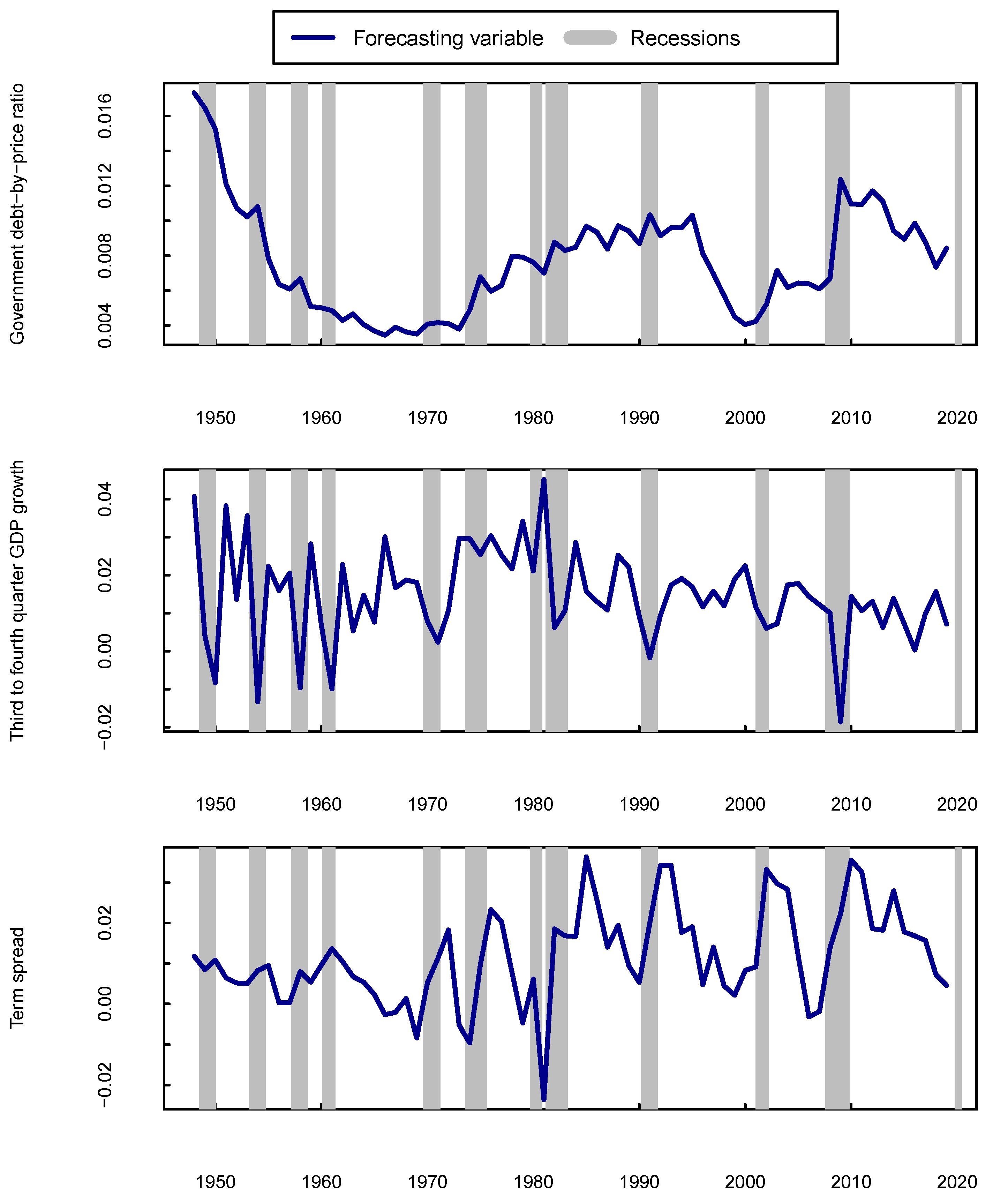
Following World War II, the United States experienced a high and steady economic growth from 1949 to 1975. This period of real growth was accompanied by a high growth of the stock market [1]. After this period, as shown in Figure 1, the economic growth has been significantly characterised by the augmentation of public debt reaching a debt-to-GDP ratio of 135.6% in the second quarter of 2020 [2]. The policies carried out to ease the Great Recession and the COVID-19 pandemic led the economy to larger amounts of debt as well as near-zero interest rates, making us ponder if the high growth on the stock market is only to a limited degree related to the real economic growth and might as well be linked to the growing debt and low interest rates. Meanwhile, the consecutive years with a low bond yield environment have been very challenging for the long-term savers see, e.g., [3]. The objective of this research is to provide a long-term forecasting approach to improve strategic asset allocation, also when interest rates are low, by investigating the hypothesis that both economic growth and government debt are risk factors priced in the time series of stock returns.

Many studies have attempted to predict stock returns using macroeconomic variables, mainly because they can affect the firm’s future cash flows by variation in the investment opportunities and consumption. Examples include default and term spreads on bonds [4]; interest rates [5,6]; inflation rate [7]; consumption–wealth ratio [8]; investment–capital ratio [9]; investment plans [10]; ratio of labor income to total income [11]; ratio of housing to total consumption [12], out-put gap [13] and end-of-year economic growth [14]. Regardless of this substantial effort, it has been empirically puzzling to find signs of macroeconomic variables when forecasting stock returns. There is a lack of robust forecasting power within macroeconomic variables, excluding the term spread, short-term interest rate and consumption–wealth ratio. The most-examined variables have been financial indicators instead of macroeconomic variables [15]. Following this line of investigation, this paper introduces a brand new variable which is the ratio of public debt to stock prices, namely, debt-by-price ratio. When debt-by-price ratio is combined with the end-of-year economic growth [14] in a multivariate setting accounts for a considerable fraction of the US stock returns variation confirming our initial hypothesis.

This work is inspired by the research on valuation ratios which connect stock prices to their cash flows, namely, dividend-by-price and earnings-by-price ratios, e.g., [17,18,19,20,21]; price-by-GDP ratio [22], which is the combination of valuation ratios and macroeconomic variables due to the belief that changes in aggregate dividends or earnings are linked with the aggregate output in the economy; the recent literature on the relationship between government debt and expected returns, e.g., [23]; the importance of information stored in the end-of-year economic growth [14].

It is historically popular that additional government debt can boost the economy in the short-term and might also trigger long-term growth since the extra spending helps the economy. On the contrary, debt can hamper the long-term economic growth on the path to recovery with rises in the inflation, tax and borrowing costs, e.g., [24,25,26]. In spite of these, the empirical literature on the relationship between fiscal policy and stock returns has been rather sparse until recently. For instance, a limited number of studies examine the impact of fiscal policy on stock prices in the Canadian and US stock markets [27,28,29]. Furthermore, a positive relationship between debt-to-GDP ratio and risk premiums for high R&D firms using the cross-section of stock returns has been confirmed [23]. In this research, by examining a long list of debt related covariates, debt-by-price ratio shows exceptional performance in forecasting US stock returns such that an increase in debt-by-price ratio is associated with a rise in excess stock returns.

Furthermore, it is stated that the end-of-year economic growth contains important information about stock returns that other quarters do not [14]. It is argued that establishing a relationship between stock returns and economic growth using all the quarters offset the end-of-year effect. By examining the forecasting power of both fourth to fourth quarter and third to fourth quarter economic growth rates in predicting one-year-ahead excess stock returns, the results of this paper support the argument that the third to fourth quarter economic growth contains such powerful information that cannot be detected from the fourth to fourth quarter growth rates. This finding exclusively holds for economic-growth related variables, namely, GDP, industrial production and consumption. On that account, annual frequency data for the remainder of the predictive variables would suffice.

The empirical findings of this paper demonstrate that debt-by-price ratio and end-of-year GDP growth are both individually strong predictors of expected returns with out-of-sample R-squared equal to 17.3% and 15.4%, respectively. Both variables contain independent information such that when combined together, the out-of-sample R-squared reaches 28% for a one-year horizon. While there is a positive relationship between debt-by-price ratio and excess stock returns, GDP growth and excess stock returns are negatively correlated. High debt-by-price ratio and low GDP growth rate relate to high equity risk premiums. While the out-of-sample R-squared of many well-known predictive variables can hardly beat the historical average [30], as evidenced by the results in this paper, the current research adds to the stock return predictability literature [15,31,32,33,34,35,36]. This new approach describing the impact of US economic growth and government debt on stock returns also adds new insights into recent methodological advances (see [35]).

The rest of the paper proceeds as follows. Section 2 explains the technical motivation. Section 3 illustrates the framework of prediction, the underlying financial model and the data. In Section 4, the results of the empirical application in different validated scenarios are demonstrated. Section 5 concludes.

2. The Technical Motivation

For the application of long-term stock returns prediction, one-year horizon models are constructed using the annual data of S&P500 index during 1947–2020. It is noteworthy that applying a data set with a small number of observations can give rise to problems related to data sparsity and overfitting, and one could suggest the use of a shorter-term frequency data to overcome this challenge. However, the bias–variance trade off is determined by the horizon and the application of prediction differs extremely for various horizons.

To avoid such problems, this paper builds on the large actuarial-predictability literature [35,36,37,38,39,40] with the intention of importing more structure in the estimation process. Initially, a validated R-squared appropriate for nonparametric prediction is introduced in an attempt to predict the Danish stock market [37]. Later on, the US stock returns in excess of risk-free rates are predicted comparing parametric, semi-parametric and nonparametric regressions [38,39]. Then, the popular forecasting variables in the literature are tested in a nonparametric setting using different benchmarks, namely, US stock returns in excess of risk-free rates; long-term interest rate; earnings-by-price ratio and inflation [36]. The extension to longer horizon prediction is subsequently studied [35]. Finally, the conditional variance of long-term stock returns for both the one and five year horizons are predicted [40]. The latter is recently mentioned in the Special Issue on “Machine Learning in Insurance” as one of the ten high-quality articles developing new theoretical or practical advances in insurance [41].

According to the literature, stock return predictability is more powerful when nonparametric models are considered, yet the linear regression is the more commonly used approach. In keeping with the studies mentioned above, a local-linear kernel smoother combined with a leave-k-out cross-validation is applied in this research. Thereafter, an out-of-sample measure of predictive power is used, as an in-sample measure such as goodness-of-fit does not prove suitable for nonparametric models. For both model and optimal bandwidth selection, the generalised version of the validated R-squared $R_V^2$, introduced by Nielsen and Sperlich [37], which measures the predictive power of a given model based on a leave-k-out cross-validation compared to the cross-validated historical mean, is applied. $R_V^2$ takes negative values when the estimated prediction model preforms worse than the cross-validated historical mean. For instance, only one- and two-dimensional models are illustrated, as all attempted three-dimensional models achieve unsatisfactory predictions. The classical $R^2$ would clearly choose the three-dimensional covariate as it tends to choose the most complicated model. We should note that the absence of prediction is not due to an inadequate model but due to the estimation error. Considering the fact that the prediction of stock returns is rather difficult, the majority of the attempted covariates result in negative $R_V^2$ values. For greater clarity, only the covariates with the highest predictive power, and a few for the purpose of comparison, are indicated; otherwise, many more covariates have been examined throughout this research.

3. Data and the Prediction Model

3.1. The Nonparametric Model

Stock returns are defined as

$$S_t=(P_t+D_t)/P_{t-1}$$

where $D_t$ denotes the (nominal) dividends paid during year t and $P_t$ the (nominal) stock price at the end of year t, in excess (log-scale) of a given benchmark $B_{t-1}^{\left(A\right)}$:

$$Y_t^{\left(A\right)}=ln\frac{S_t}{B_{t-1}^{\left(A\right)}}$$

(1)

where $A\in \{R,L,E,C\}$ with, respectively,

$$B_t^{\left(R\right)}=1+\frac{R_t}{100},B_t^{\left(L\right)}=1+\frac{L_t}{100},B_t^{\left(E\right)}=1+\frac{E_t}{P_t},B_t^{\left(C\right)}=\frac{CP{I}_t}{CP{I}_{t-1}},$$

$R_t$ is the short-term interest rate, $L_t$ the long-term interest rate, $E_t$ the earnings accruing to the index in year t, and $CP{I}_t$ the consumer price index for year t.

The nonparametric regression model for the one-year horizon prediction is then given by

$$Y_t^{\left(A\right)}=m\left(X_{t-1}\right)+{\xi }_t,$$

(2)

where the conditional mean $m\left(x\right)=\mathbb{E}\left(Y^{\left(A\right)}\right|X=x),x\in {\mathbb{R}}^q$, is an unknown smooth function and ${\xi }_t$ a martingale difference process, i.e., has serially uncorrelated zero-mean random error terms, given the past, of an unknown conditionally heteroscedastic form $\sigma \left(x\right)$.

We predict one-year horizon excess stock returns by applying a local-linear kernel smoother using a quartic kernel where the optimal bandwidth, and consequently the best model, is chosen by cross-validation. Provided that a local-linear smoother is used, the model can estimate linear functions without any bias and the linear regression is embedded by design in this approach. Longer horizon predictions can also be incorporated in the analysis with the sum of annual continuously compounded returns, $Z_t^{\left(A\right)}={\sum }_{i=0}^{T-1}{Y}_{t+i}^{\left(A\right)}$. Further details regarding the nonparametric regression and its extension to longer horizon predictions are included in Kyriakou et al. [35,36].

This paper attempts to forecast one-year-ahead excess stock returns $Y_t^{\left(A\right)}$ measured over the calendar year using the time-lagged macroeconomic variables $X_{t-1}$ related to government debt and economic growth. A few of these variables are demonstrated in

Table 1. Time-lagged predictive variables $X_{t-1}$ related to government debt and economic growth. Q/Q is the quarter-over-quarter growth rate from the third to the fourth quarter of a year, GDP is the nominal gross domestic product, IP the industrial production index, CON nominal personal consumption expenditures and DEB the total government debt.

Predictive Variables	${\mathit{X}}_{\mathit{t}-1}$
Growth in GDP (Q/Q)	$gd{p}_{t-1}=(GD{P}_{t-2}^{Q4}-GD{P}_{t-2}^{Q3})/GD{P}_{t-2}^{Q3}$
Growth in industrial production (Q/Q)	$i{p}_{t-1}=(I{P}_{t-2}^{Q4}-I{P}_{t-2}^{Q3})/I{P}_{t-2}^{Q3}$
Growth in personal consumption expenditures (Q/Q)	$co{n}_{t-1}=(CO{N}_{t-2}^{Q4}-CO{N}_{t-2}^{Q3})/CO{N}_{t-2}^{Q3}$
GDP-by-price ratio	$gp{r}_{t-1}=GD{P}_{t-1}/P_{t-1}$
Debt-by-price ratio	$dp{r}_{t-1}=DE{B}_{t-1}/P_{t-1}$
Debt-by-GDP ratio	$dg{r}_{t-1}=DE{B}_{t-1}/GD{P}_{t-1}$

; otherwise, many more variables have been examined. For the purpose of comparison, year-over-year growth rates as well as popular predictive variables in the literature are also illustrated, namely, dividend-by-price ratio $d_{t-1}=D_{t-1}/P_{t-1}$; earnings-by-price ratio $e_{t-1}=E_{t-1}/P_{t-1}$; short-term interest rate $r_{t-1}=R_{t-1}/100$; long-term interest rate $l_{t-1}=L_{t-1}/100$; inflation ${\pi }_{t-1}=(CP{I}_{t-1}-CP{I}_{t-2})/CP{I}_{t-2}$; term spread $s_{t-1}=l_{t-1}-r_{t-1}$; the consumption–wealth ratio ${\widehat{cay}}_{t-1}$ [8].

3.2. Out-of-Sample Validation for Optimal Model and Bandwidth Selection

Since a nonparametric regression is applied in this research, classical in-sample measures such as $R^2$ or adjusted $R^2$ are not appropriate. Thus, the generalised version of the validated $R^2$$\left(R_V^2\right)$ [37], a suitable out-of-sample measure, is used in order to determine the forecasting power of the nonparametric models. This method is based on a leave-k-out cross-validation and is employed for both model and bandwidth selection. Cross-validation is an advantageous measure for preventing the occurrence of overfitting as well as for finding the optimal bandwidth for non- and semi-parametric estimators, e.g., [42]. $R_V^2$ measures the predictive power of a given model compared to the cross-validated historical mean; positive $R_V^2$ implies that the predictor-based regression model (2) outperforms the corresponding historical average excess stock returns.

The validation criterion is defined as

$$R_V^2=1-\frac{{\displaystyle \sum _t}{(Y_t^{\left(A\right)}-{\widehat{m}}_{-t})}^2}{{\displaystyle \sum _t}{(Y_t^{\left(A\right)}-{\overline{Y}}_{-t}^{\left(A\right)})}^2},$$

(3)

where leave-k-out estimators are used: ${\widehat{m}}_{-t}$ for the nonparametric function m and ${\overline{Y}}_{-t}^{\left(A\right)}$ for the unconditional mean of $Y_t^{\left(A\right)}$. Both are computed by removing k observations around the tth time point where $k=2T-1$. For example, in the one-year horizon application, the classical leave-one-out estimator is used because of the construction of the dependent variable over a horizon of one year $(T=1)$.

Additionally, the forecasting power of nominal stock returns $lnS$ is measured by back-transforming the prediction models of benchmarked excess stock returns in order to make the results comparable for the different benchmarks. It should be acknowledged that prediction based on different benchmarks has its own merits. For instance, the short-term interest rate is beneficial for classical market-timing strategies or the inflation benchmark for wealth and purchasing power problems of long-term investment planning see, e.g., [43].

The stock return in excess of benchmark A is

$$Y_t^{\left(A\right)}=ln{S}_t-ln{B}_{t-1}^{\left(A\right)}$$

Then, the back-transformed stock return prediction is defined as

$$\widehat{ln{S}_t}={\widehat{Y}}_t^{\left(A\right)}+ln{B}_{t-1}^{\left(A\right)},$$

(4)

where $\widehat{Y}$ is the predicted benchmarked excess return, and we redefine our original validation criterion (3) as

$${\tilde{R}}_V^2=1-\frac{{\displaystyle \sum _t}{\left(ln{S}_t-{\left(\widehat{lnS}\right)}_{-t}\right)}^2}{{\displaystyle \sum _t}{\left(ln{S}_t-{\left(\overline{lnS}\right)}_{-t}\right)}^2},$$

(5)

where ${\left(\widehat{lnS}\right)}_{-t}$ is the back-transformed stock return prediction from the original leave-one-out benchmarked return prediction and ${\left(\overline{lnS}\right)}_{-t}$ the unconditional mean of $lnS$. This allows us to validate in terms of $R_V^2$ with the observed $ln{S}_t$. There is a fundamental difference between Equations (3) and (5). Equation (3) chooses the optimal bandwidth and, subsequently, the predictive model via cross-validation. However, Equation (5) is not based on cross-validation and applies the bandwidths chosen in Equation (3) only to measure the predictive power of nominal returns for different benchmarking scenarios. When the main goal of the prediction is the nominal stock returns, one would cross-validate directly.

3.3. Data

The empirical analysis in this research attempts to connect government debt and economic growth data to stock returns stressing on the long-term actuarial predictability. The prediction models cover the sample period from 1947 to 2020 since the quarterly national accounts are only available from 1947.

Annual and quarterly frequency data of seasonally adjusted nominal gross domestic product (GDP) and nominal personal consumption expenditures are extracted from the U.S. Bureau of Economic Analysis [44]. Furthermore, the seasonally adjusted industrial production index is obtained from the Federal Reserve Economic Data (FRED) database of the Federal Reserve Bank of St. Louis [45]. The nominal total public debt (not seasonally adjusted) is downloadable from the U.S. Department of the Treasury Bureau of the Fiscal Service database [46]. It should be noted that seasonality has not been detected in the debt series and no seasonal adjustments have been done. Furthermore, the GDP, consumption expenditures, and government debt are measured in trillions of dollars. The rest of the financial data is available from Robert Shiller’s website [47] which, for a given year, offers the January value of the Standard and Poor’s Composite Stock Price Index, the value of the related dividends and earnings, consumer price index, and interest rate data. The short-term interest rate from Shiller’s website is based on a 6-month commercial paper rate until 1997 and subsequently on the 6-month certificate of deposit rate which is no longer available after 2013. This series is substituted by an annual yield based on the six-month Treasury-bill rate from 1958 to 2020 [48], and prior to this period the estimations by Kyriakou et al. [35] using the regressions of Treasury-bill rate on the risk-free rate from Shiller’s data for the overlapping period 1958–2013 have been used. Finally, the alth ratio has been downloaded from Amit Goyal’s webpage [49].

Table 2. The table shows the summary statistics for the dependent and forecasting variables. $Y^{\left(R\right)}$ is the stock return in excess of risk free rate; gdp the third to fourth quarter GDP growth; ip the third to fourth quarter industrial production growth; con the third to fourth quarter consumption growth; gpr the GDP-by-price ratio; dpr the debt-by-price ratio and dgr the debt-by-GDP ratio. The sample period is 1947–2020.

	${\mathit{Y}}^{\left(\mathit{R}\right)}$	gdp	ip	con	gpr	dpr	dgr
Mean	6.49	1.47	0.82	1.46	1.36	0.76	59.5
Standard deviation	15.41	1.20	2.01	0.99	0.52	0.3	22.14

reports the mean and standard deviation for the one-year excess stock returns and the forecasting variables introduced in Table 1. In Figure 2, the most successful forecasting variables in this analysis are plotted in an attempt to detect the elements of expected returns they could demonstrate. Debt-by-price ratio, third to fourth quarter GDP growth and term spread alongside business cycles measured by the NBER [50] covering 1947–2020 are demonstrated. Term spread is historically known as a good predictor of the stock market and is widely recognised to contain information about shorter-term business cycles [4,35,36,51]. It is also one of the outstanding predictors amongst the regression models in this paper. While the debt-by-price ratio demonstrates some business cycle fluctuations with an increase near the peaks and a decrease near the troughs during almost all the recessions, its overall fluctuations seem to be persistent over the years, and contain signals about the longer-term business conditions that tend to persist. On the other hand, the GDP growth and the term spread fluctuations are mainly near business peaks and troughs. It appears that both similarly contain information about short-term fluctuations and recessions.

4. The Empirical Application

4.1. The Relationship between Stock Returns and Government Debt

The present value model which relates stock prices to their expected future cash flows based on the dynamic generalisation of the Gordon growth model states that log dividend–price ratio $d_t-p_t$ can be written as discounted value of all future returns $r_{t+j}$ and dividend growth rates $\Delta d_{t+j}$ discounted at the constant rate $\rho$ see, e.g., [19,20,52]. This model is derived by taking a first-order Taylor approximation of the equation defining the log stock returns $s_t=log(P_t+D_t)/P_{t-1}$

$$d_t-p_t={\mathbb{E}}_t\sum _{j=1}^{+\infty }{\rho }^j(r_{t+j}-\Delta d_{t+j})+k,$$

(6)

where ${\mathbb{E}}_t$ is the expectation operator conditional on the information at time t, $\rho \equiv 1/(1+exp\left(\overline{d-p}\right))$, $\overline{d-p}$ is the mean log dividend-price ratio and k is a constant.

Equation (6) by ruling out the rational bubbles demonstrates the possibility of capturing the expectations of investors by examining the change in the dividend-price ratio. When the stock prices are high for the given dividends, stock market participants ought to be expecting either high dividend growth rates or low returns on the assets and vice versa. Nevertheless, the importance of valuation ratios has been less in forecasting stock returns in recent years [15,53,54]. It is demonstrated that the relationship between dividend yields and future stock returns is cancelled out with the time-varying expected dividend growth [11]. Furthermore, it is found that the dividend-by-price ratio fails to predict the fluctuations in expected returns and dividend growth due to the offsetting effect of positively correlated movements [55], originating the question whether there is another variable that can explain the movements in stock returns in a way that can also predict this offsetting component. For example, the consumption–wealth ratio and price-to-GDP ratio are introduced in an attempt to find this unknown covatiate [8,22].

Alternatively, in this research, after examining many debt-related variables, such as government debt, budget deficit, debt-to-GDP ratio and their associated growth rates, the debt-by-price ratio is proposed. This consideration is based on the fact that government debt is the main function of the current economy, and it is probably the main determinant of the variation in expected returns. It is worth noting that dividing by prices is just a practical method to detrend the government debt series and what matters is the high levels of government debt.

According to Equation (6), what could be happening is that in times of financial uncertainty and rising levels of government debt, investors consider the market risky possibly because of the anticipated increase in tax payments, lower cash flows, decline in economic growth, and generally the elevated fiscal uncertainty. Hence, they panic, sell and bring down the share prices which accordingly increases the expected returns. The government’s money injection in the economy in order to overcome the hardship comes into force eventually via the positive relationship of the government debt with stock prices and dividends payout, and the investors who bought low can reap the rewards.

Government debt can positively affect stock prices and dividends payout for a few possible reasons. First, the government debt can affect firms’ dividends payout as companies have become more friendly towards shareholders, returning more of their earnings in the form of dividends and stock buybacks even if they are burdened with debt. Second, the increased stock buybacks can inflate the companies’ stock prices artificially. Third, the government debt can stimulate GDP growth by investing in the company and creating more jobs; also the stockholders’ gains from the share buybacks can be reinvested in other companies, hence increase the stock prices. Fourth, high levels of government debt are usually associated with low interest rates, which pressure the investors to move their money from the bond to the equity market and, as a result, amplify stock prices.

On the other hand, it is possible that there is a simpler explanation beyond such asset pricing models. The authors of [56] picture the history of the last several hundred years filled with credit cycles. It is explained that some structural change leads to a change in the amount of money and a massive credit boom, followed by an asset boom in the domestic markets which encourages investors for risky investments, and they will continue investing in the markets as those investments pay off. At some point, the capital flow reaches the foreign lands from the starting markets. Finally, the expansion ends even more unexpectedly than when it started. It appears that, throughout history, credit booms—or, to put it more bluntly, pumping liquidity into the economy—have been the real reason behind the stock market booms.

Univariate Regressions of Stock Returns on Price Ratios

Table 3. Predictive power for the one-year excess stock returns $Y_t^{\left(A\right)}$. The prediction problem is defined in (2). The predictive power (%) is measured by $R_V^2$ as defined in (3). The benchmarks $B^{\left(A\right)}$ considered are based on the short-term interest rate ($A\equiv R$), long-term interest rate ($A\equiv L$), earnings-by-price ratio ($A\equiv E$), and consumer price index ($A\equiv C$). The predictive variables $X_{t-1}$ used are given by dividend-by-price ratio $d_{t-1}$, earnings-by-price ratio $e_{t-1}$, debt-by-price ratio $dp{r}_{t-1}$ and GDP-by-price ratio $gp{r}_{t-1}$. The predictive power (%) for the one-year stock returns $ln{S}_t$ validated on the original scale without benchmark is measured by ${\tilde{R}}_V^2$ as defined in (5) in terms of back-transformed stock return prediction $\widehat{ln{S}_t}$ defined in (4). The sample period is 1947–2020.

Benchmark ${\mathit{B}}^{\mathit{A}}$	${\mathit{X}}_{\mathit{t}-1}$
	${\mathit{R}}_{\mathit{V}}^{\mathbf{2}}$				${\tilde{\mathit{R}}}_{\mathit{V}}^{\mathbf{2}}$
	d	e	dpr	gpr	d	e	dpr	gpr
Short-term rate	4.1	0.7	17.3	0.34	−2.1	−5.8	11.9	−6.15
Long-term rate	5.1	1.6	15.1	0.17	2.4	−1.3	12.6	−2.70
Earnings-by-price	0.1	−1.9	10.7	0.31	6.2	4.4	16.2	6.44
Inflation	3.0	−0.3	13.3	0.50	−1.9	−5.4	8.8	1.76

reports $R_V^2$ values based on the univariate regressions of excess stock returns on dividend-by-price ratio, earnings-by-price ratio, debt-by-price ratio and GDP-by-price ratio under different benchmarks, and the corresponding ${\tilde{R}}_V^2$ values related to the prediction of stock returns $ln{S}_t$ validated on the original scale without benchmark in terms of back-transformed stock return prediction $\widehat{ln{S}_t}$.

The results confirm the literature that casts doubts about the predictive power of dividend-by-price or earnings-by-price ratios. While earnings-by-price ratio $\left(e\right)$ shows low explanatory power under all the benchmarks with $R_V^2$ in the range of −1.9–1.6% and ${\tilde{R}}_V^2$ in the range of −5.8–4.4%, dividend-by-price ratio $\left(d\right)$ can at the most explain 5.1% variation of stock returns in excess of short-term rate with $R_V^2$ in the range of 0.1–4.1% under the remaining of the benchmarks and ${\tilde{R}}_V^2$ in the range of −2.1–6.2%. The GDP-by-price ratio $\left(gpr\right)$ also does not look promising with $R_V^2$ in the range of 0.17–0.5% and ${\tilde{R}}_V^2$ in the range of −6.15–6.44%. All of these variables perform acceptably in the prediction of nominal stock returns under the earnings-by-price benchmark. This is not unanticipated, as earnings-by-price ratio is regularly used as a return measure by investors and provides an adequate understanding of an investment return. On the other hand, the debt-by-price ratio $\left(dpr\right)$ performance is remarkable with $R_V^2=17.3\%$ under the risk-free rate benchmark and ${\tilde{R}}_V^2=16.2\%$ under the earnings-by-price benchmark. It also appears to be a powerful predictive variable with regards to the other benchmarks with $R_V^2=15.1\%$, 10.7% and 13.3% under the long-term rate, earnings-by-price and inflation benchmarks, and ${\tilde{R}}_V^2=11.9\%$, 12.6% and 8.8% under the short-term rate, long-term rate and inflation benchmarks.

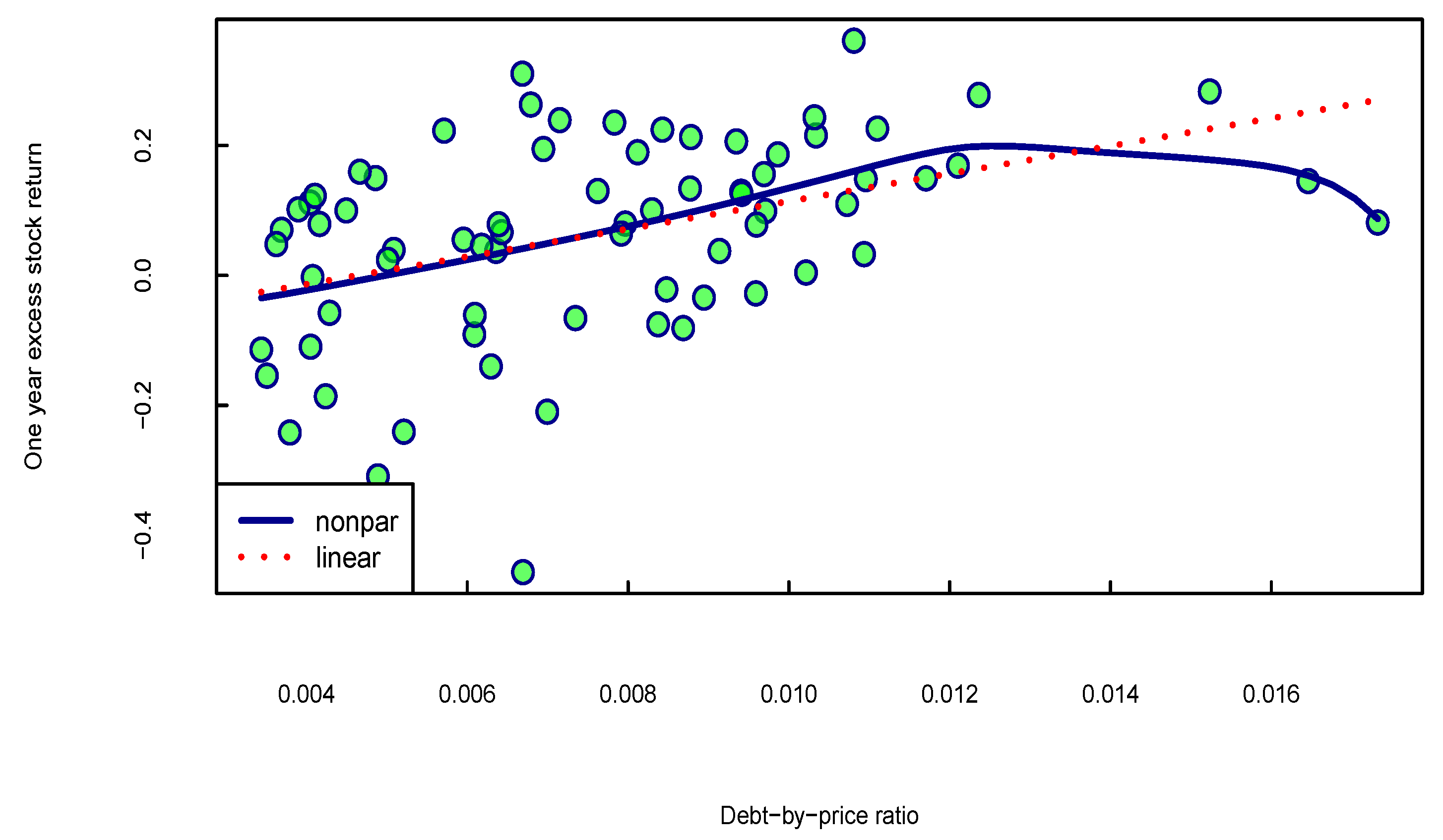
Figure 3 demonstrates the estimated function $\widehat{m}$ (dark blue line) for the one-year horizon together with a corresponding linear model (dotted red line). The figure confirms that an increase in the debt-by-price ratio corresponds to an increase in the stock returns. In general, a debt-by-price ratio of more than 0.5% forecasts a positive return of up to almost 20% for a debt-by-price ratio of 1.25%. Excluding the two outliers which belong to the post-war period of 1947–1948, using the risk-free benchmark then the functional form can be written as a simple line:

$$\begin{array}{c}\hfill \mathrm{One-year}\mathrm{excess}\mathrm{stock}\mathrm{return}=-0.09874+21.27971\times \mathrm{Debt-by-price}.\end{array}$$

(7)

Equation (7) simply illustrates that when 2027.971% is added to the government debt divided by the stock price plus −9.874% equals the one-year ahead expected return.

4.2. Third to Fourth Quarter Economic Growth

In this section, the predictive power of both the third to fourth quarter and the fourth to fourth quarter (annual) growth rates of GDP, industrial production and consumption in forecasting stock returns are studied. Different economic growth variables are applied, establishing the fact that the results are not guided by chance. It must be pointed out that only the third to fourth and the fourth to fourth quarter growth rates are examined as the one-year ahead excess stock return measured over the calendar year is the target of the prediction.

Møller and Rangvid [14] analyze the first, second, third and fourth quarter growth rates of economic growth to predict one-year ahead excess stock returns, and indicate that except the fourth quarter economic growth rate, other quarters do not affect the expected returns significantly. They also examine the fourth to fourth versus the third to fourth quarter growth rates, and show that the third to fourth quarter growth rates contain much more information than the fourth to fourth quarter growth rates. They argue that investors are lazy [57] and make portfolio decisions about expected returns mostly at the the end of the year [58,59] because of information and transaction costs [60]. Moreover, extensive macroeconomic fluctuations around the end of the year result in large business cycle variations [61] which causes the investors to take this huge end-of-the-year economic growth into consideration [62]. This argument fairly summarizes the economic intuition behind the fact that expected returns are more affected by the third to fourth quarter growth rates.

Univariate Regressions of Stock Returns on Economic Growth

Table 4. Predictive power for the one-year excess stock returns $Y_t^{\left(A\right)}$. The prediction problem is defined in (2). The predictive power (%) is measured by $R_V^2$ as defined in (3). The benchmarks $B^{\left(A\right)}$ considered are based on the short-term interest rate ($A\equiv R$), long-term interest rate ($A\equiv L$), earnings-by-price ratio ($A\equiv E$), and consumer price index ($A\equiv C$). The predictive variables $X_{t-1}$ used on Panel A are given by the third to fourth quarter growth rates of GDP $gd{p}_{t-1}$, industrial production $i{p}_{t-1}$ and personal consumption expenditures $co{n}_{t-1}$. Panel B shows the fourth to fourth quarter (annual) growth rates of these corresponding variables. The predictive power (%) for the one-year stock returns $ln{S}_t$ validated on the original scale without benchmark is measured by ${\tilde{R}}_V^2$ as defined in (5) in terms of back-transformed stock return prediction $\widehat{ln{S}_t}$ defined in (4). The sample period is 1947–2020.

Benchmark ${\mathit{B}}^{\mathit{A}}$	${\mathit{X}}_{\mathit{t}-1}$
	${\mathit{R}}_{\mathit{V}}^{\mathbf{2}}$			${\tilde{\mathit{R}}}_{\mathit{V}}^{\mathbf{2}}$
	gdp	ip	con	gdp	ip	con
Panel A: Third to fourth quarter
growth rate
Short-term rate	15.4	15.7	17.3	9.9	10.2	11.9
Long-term rate	14.5	15.2	16.2	12.1	12.8	13.8
Earnings-by-price	15.7	14.9	15.2	20.9	20.1	20.5
Inflation	17.2	13.3	14.6	13.0	8.9	10.2
Panel B: Fourth to fourth quarter
growth rate
Short-term rate	−0.4	1.0	−5.9	−6.9	−5.4	−12.8
Long-term rate	−1.2	0.9	−5.9	−4.1	−1.9	−8.9
Earnings-by-price	−0.3	0.8	−5.9	5.9	6.9	0.6
Inflation	−0.2	3.0	−6.0	−5.3	−2.0	−11.4

demonstrates $R_V^2$ values based on the univariate regressions of excess stock returns on the third to fourth quarter and the fourth to fourth quarter (annual) economic growth rates of GDP, industrial production and consumption under different benchmarks, and the corresponding ${\tilde{R}}_V^2$ values related to the prediction of stock returns $ln{S}_t$ validated on the original scale without benchmark in terms of back-transformed stock return prediction $\widehat{ln{S}_t}$.

The results in Panel A illustrate a robust relationship between the third to fourth quarter economic growth variables and both excess and nominal stock returns under all the benchmarks with $R_V^2$ in the range of 13.3–17.3% and ${\tilde{R}}_V^2$ in the range of 8.9–20.9%. It is notable that all the third to fourth quarter economic growth rates achieve high $R_V^2$ values. GDP $\left(gdp\right)$ performs the best under the inflation benchmark with $R_V^2=17.2\%$, but also does well under the short-term rate, long-term rate and earnings-by-price benchmarks with $R_V^2=15.4\%$, 14.5% and 15.7%, respectively. Consumption $\left(con\right)$ is the leading predictor under the short-term rate benchmark with $R_V^2=17.3\%$, and $R_V^2$ in the range of 14.6–16.2% under the remainder of the benchmarks. $R_V^2$ values related to industrial production $\left(ip\right)$ remain moderately similar within the range 13.3–15.7%. The values related to nominal stock returns tell a slightly different story. While the forecasting power of GDP $\left(gdp\right)$, industrial production $\left(ip\right)$ and consumption $\left(con\right)$ is reasonable under the short-term rate, long-term rate and inflation benchmarks with, respectively, ${\tilde{R}}_V^2$ in the ranges of 9.9–13%, 8.9–12.8% and 10.2–13.8%, the case of the earnings-by-price benchmark is remarkable, leading to ${\tilde{R}}_V^2$ in the range of 20.1–20.9%.

On the other hand, as demonstrated in Panel B, the fourth to fourth quarter economic growth rates are not promising to any extent. GDP $\left(gdp\right)$ and consumption $\left(con\right)$ result in negative $R_V^2$ values under any benchmark, and industrial production $\left(ip\right)$ shows minor signs of forecasting power with $R_V^2$ in the range of 0.8–3.0%. In addition, earnings-by-price is the only benchmark that results in positive ${\tilde{R}}_V^2$ values in the range of 0.6–6.9% in prediction of nominal stock returns.

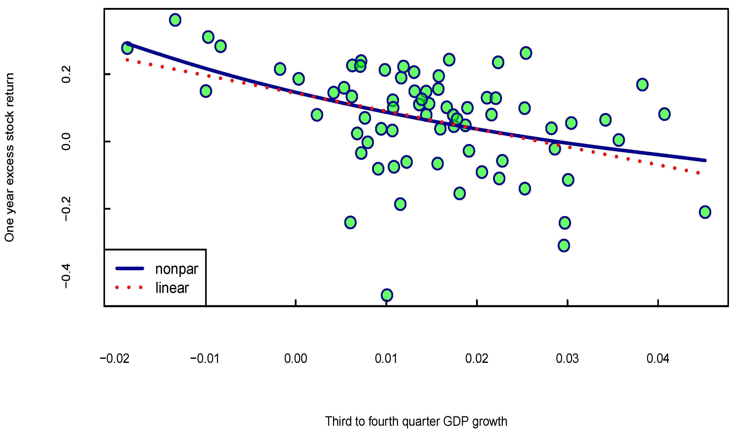
Overall, these findings confirm the fact that the third to fourth quarter growth rates contain such powerful information about the stock returns which, when the fourth to fourth quarter growth rates are used, this information fades away with the noise existing in the other quarters. It should be pointed out that both seasonally adjusted and not seasonally adjusted data were examined during this analysis, and it is by removing the seasonality that the excellent performance of the third to fourth quarter growth rates comes into effect. As is clear from Figure 4, there is a negative relationship between the third to fourth quarter GDP growth and the excess returns, forecasting positive excess returns for a GDP growth rate of less than 3%. This outcome is in line with the hypothesis of the variation of excess returns with business cycles; for instance, investors’ unwillingness to invest during the recessions increases the expected returns [62].

4.3. More Macroeconomic Variables

Table 5. Predictive power for the one-year excess stock returns $Y_t^{\left(A\right)}$. The prediction problem is defined in (2). The predictive power (%) is measured by $R_V^2$ as defined in (3). The benchmarks $B^{\left(A\right)}$ considered are based on the short-term interest rate ($A\equiv R$), long-term interest rate ($A\equiv L$), earnings-by-price ratio ($A\equiv E$), and consumer price index ($A\equiv C$). The predictive variables $X_{t-1}$ used are given by the short-term interest rate $r_{t-1}$, long-term interest rate $l_{t-1}$, inflation ${\pi }_{t-1}$, term spread $s_{t-1}$, debt-by-GDP ratio $dg{r}_{t-1}$ and consumption–wealth ratio ${\widehat{cay}}_{t-1}$. The predictive power (%) for the one-year stock returns $ln{S}_t$ validated on the original scale without benchmark is measured by ${\tilde{R}}_V^2$ as defined in (5) in terms of back-transformed stock return prediction $\widehat{ln{S}_t}$ defined in (4). The sample period is 1947–2020.

Benchmark ${\mathit{B}}^{\mathit{A}}$	${\mathit{X}}_{\mathit{t}-1}$
	${\mathit{R}}_{\mathit{V}}^{\mathbf{2}}$						${\tilde{\mathit{R}}}_{\mathit{V}}^{\mathbf{2}}$
	r	l	$\mathbf{\pi }$	s	dgr	$\widehat{\mathbf{cay}}$	r	l	$\mathbf{\pi }$	s	dgr	$\widehat{\mathbf{cay}}$
Short-term rate	3.7	2.1	−1.0	11.4	6.9	3.0	−2.6	−4.3	−7.6	5.6	0.9	−3.2
Long-term rate	2.6	2.4	−1.0	8.3	6.0	3.7	−0.2	−0.4	−3.9	5.7	3.3	0.9
Earnings-by-price	−0.8	−1.7	−1.6	8.7	1.7	0.0	5.4	4.6	4.6	14.3	7.8	6.1
Inflation	0.5	0.0	1.7	9.6	3.7	3.8	−4.6	−5.1	−3.3	5.0	−1.3	−1.2

displays, for the sake of comparison, $R_V^2$ values based on the univariate regressions of excess stock returns on a couple of well-known predictive variables in the literature such as the short-term interest rate, long-term interest rate, inflation, term spread, debt-by-GDP ratio and consumption–wealth ratio under various benchmarks, and the corresponding ${\tilde{R}}_V^2$ values related to the prediction of stock returns $ln{S}_t$ validated on the original scale without benchmark in terms of back-transformed stock return prediction $\widehat{ln{S}_t}$.

All in all, the term spread $\left(s\right)$ is the most important predictor with $R_V^2=11.4\%$ under the short-term benchmark and ${\tilde{R}}_V^2=14.3\%$ under the earnings-by-price benchmark, but also performs reasonably under the different benchmarks with $R_V^2$ and ${\tilde{R}}_V^2$ in the ranges of 8.3–9.6% and 5.0–5.7%, respectively. 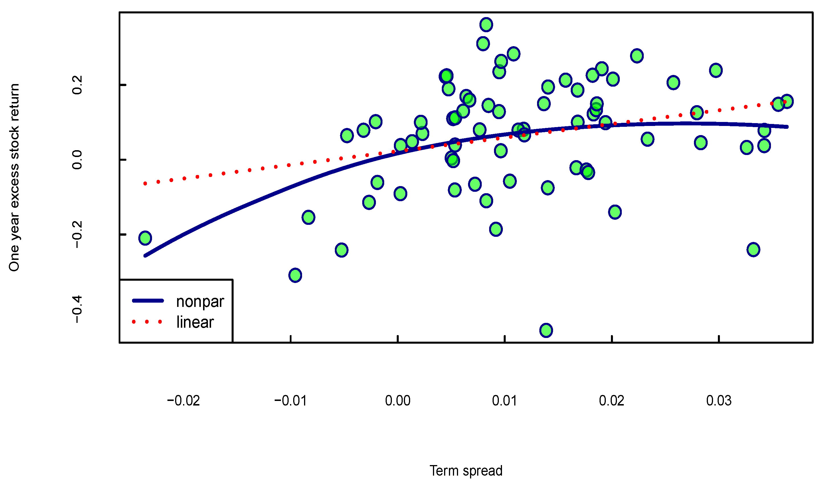This is consistent with the previous work of the authors of [35,36] where the term spread is the most favourable variable explaining the excess returns in the univariate setting with $R_V^2$ in the range of 6.2–9.7% for the sample period 1872–2019. As shown in Figure 5, the term spread signals crucial information about the possibility of a bear stock market, any term spread less than −0.3% yields negative returns.

The debt-by-GDP ratio $\left(dgr\right)$ which has been mostly applied in the literature on forecasting stock returns emphasizing on government debt can at most explain 6.9% variation of excess returns under the risk-free rate benchmark, and 7.8% variation of nominal returns under the earnings-by-price benchmark. Under the long-term rate, earnings-by-price and inflation benchmarks, the performance of this covariate declines to $R_V^2=6.0\%$, 1.7% and 3.7%, respectively. ${\tilde{R}}_V^2$ values also result in lower predictive power under the different benchmarks within the range of −1.3–3.3%.

It comes to our attention that other covariates cannot forecast stock returns with remarkable $R_V^2$ and ${\tilde{R}}_V^2$ values. The well-known consumption–wealth ratio $\left(\widehat{cay}\right)$ can only explain the variation of excess returns with $R_V^2=3.0\%$, 3.7% and 3.8% under the short-term rate, long term rate and inflation benchmarks, respectively. The short-term interest rate $\left(r\right)$ accounts for the variation of excess returns with $R_V^2=3.7\%$ under the short-term rate benchmark and $R_V^2=2.6\%$ under the long-term rate benchmark. Likewise, the long-term interest rate $\left(l\right)$ results in $R_V^2$ of 2.1% and 2.4% under the same benchmarks. Inflation $\left(\pi \right)$ demonstrates almost no signs of prediction power with $R_V^2$ in the range of −1.6–1.7%. Finally, the predictive power of the earnings-by-price ratio benchmark in prediction of nominal stock returns has been, once more, highlighted with, respectively, ${\tilde{R}}_V^2=5.4\%$, 4.6%, 4.6% and 6.1% for the covariates r, l, $\pi$ and $\widehat{cay}$.

A few more interesting comments are in order. The term spread is extensively known to contain robust information about prediction of stock returns. While this holds true in this analysis, term spread also proves to be a very consistent predictive variable as it predicts excess returns with comparable $R_V^2$ values in different sample periods. Furthermore, the reasonable predictive power of debt-by-GDP ratio confirms our findings about the importance of government debt in forecasting US stock returns.

4.4. The Multivariate Setting

Table 6. Predictive power for the one-year excess stock returns $Y_t^{\left(A\right)}$ in a two-dimensional setting. The prediction problem is defined in (2). The predictive power (%) is measured by $R_V^2$ as defined in (3). The benchmarks $B^{\left(A\right)}$ considered are based on the short-term interest rate ($A\equiv R$), long-term interest rate ($A\equiv L$), earnings-by-price ratio ($A\equiv E$), and consumer price index ($A\equiv C$). The different pairwise combinations of predictive variables, $X_{t-1}$ are given by the combination of third to fourth quarter growth rates of GDP $gd{p}_{t-1}$, industrial production $i{p}_{t-1}$ and personal consumption expenditures $co{n}_t-1$ with dividend-by-price ratio $d_{t-1}$, earnings-by-price ratio $e_{t-1}$, term spread $s_{t-1}$ and debt-by-price ratio $dp{r}_{t-1}$. The predictive power (%) for the one-year stock returns $ln{S}_t$ validated on the original scale without benchmark is measured by ${\tilde{R}}_V^2$ as defined in (5) in terms of back-transformed stock return prediction $\widehat{ln{S}_t}$ defined in (4). The sample period is 1947–2020.

Benchmark ${\mathit{B}}^{\mathit{A}}$	${\mathit{X}}_{\mathit{t}-1}$
	${\mathit{R}}_{\mathit{V}}^{\mathbf{2}}$				${\tilde{\mathit{R}}}_{\mathit{V}}^{\mathbf{2}}$
	(gdp, d)	(gdp, e)	(gdp, s)	(gdp, dpr)	(gdp, d)	(gdp, e)	(gdp, s)	(gdp, dpr)
Short-term rate	25.3	23.0	23.4	28.6	20.4	18.0	18.4	23.9
Long-term rate	24.8	22.9	20.6	25.9	22.7	20.6	18.3	23.8
Earnings-by-price	18.7	17.5	18.3	23.8	23.7	22.6	23.3	28.5
Inflation	25.2	23.9	22.1	26.2	21.3	20.0	18.1	22.4
	(ip, d)	(ip, e)	(ip, s)	(ip, dpr)	(ip, d)	(ip, e)	(ip, s)	(ip, dpr)
Short-term rate	16.3	13.9	20.7	25.4	10.9	8.3	15.6	20.5
Long-term rate	17.2	13.6	18.0	23.2	14.8	11.2	15.6	21.0
Earnings-by-price	13.6	11.6	17.6	19.9	18.9	17.1	22.7	24.8
Inflation	13.8	11.3	17.6	19.9	9.4	6.8	13.3	15.8
	(con, d)	(con, e)	(con, s)	(con, dpr)	(con, d)	(con, e)	(con, s)	(con, dpr)
Short-term rate	24.3	22.4	19.3	25.9	19.3	17.3	14.1	21.1
Long-term rate	24.1	22.4	16.5	23.7	21.9	20.2	14.1	21.6
Earnings-by-price	16.7	15.5	15.8	18.2	21.9	20.7	21.0	23.2
Inflation	19.3	17.2	15.4	19.6	15.2	13.0	11.1	15.5

illustrates a few of the best two-dimensional models, namely, the multivariate regressions of excess stock returns on the combinations of third to fourth quarter growth rates of GDP, industrial production and consumption with the dividend-by-price ratio, earnings-by-price ratio, term spread and debt-by-price ratio. More specifically, many more combinations with a reasonable forecasting power have been obtained throughout this research, however, only the best models are demonstrated. We can observe that the predictive power of two-dimensional models are higher compared to the one-dimensional cases. It must be underlined that only one- and two-dimensional models are the main focus of this analysis, as all the attempted three-dimensional models have resulted in unsatisfactory $R_V^2$ values. This is anticipated, as a nonparametric model requires more observations than a linear regression to achieve reliable estimates when dealing with higher-dimensional models.

The case of the predictor GDP $\left(gdp\right)$ is impressive; combining this with any of the covariates d, e, s and $dpr$ results in the highest $R_V^2$ values in the ranges of 18.7–25.3%, 17.5–23.9%, 18.3–23.4% and 23.8–28.6%, and ${\tilde{R}}_V^2$ values in the ranges of 20.4–23.7%, 18–22.6%, 18.1–23.3% and 22.4–28.5% under different benchmarks. Clearly, the combination of GDP and debt-by-price ratio (gdp, dpr) is the ultimate winner with $R_V^2=28.6\%$, 25.9%, 23.8% and 26.2% and ${\tilde{R}}_V^2=23.9\%$, 23.8%, 28.5% and 22.4% under the short-term rate, long-term rate, earnings-by-price and inflation benchmarks, respectively. The second best is (gdp, d) with $R_V^2=25.3\%$ and 25.2% under the short-term rate and inflation benchmarks, and ${\tilde{R}}_V^2=23.7$ under the earnings-by-price benchmark.

The two-dimensional combinations of industrial production $\left(ip\right)$ and consumption $\left(con\right)$ bring about lower predictive power than the previous ranges. The best combinations $(ip,dpr)$ and $(con,dpr)$ although resulting in $R_V^2$ within the range of 19.9–25.4% and 18.2–25.9%, still perform worse. We find that consumption $\left(con\right)$ performs much better than industrial production $\left(ip\right)$ when put together with the other covariates excluding the term spread $\left(s\right)$. Notable contributions are $(con,d)$, $(con,e)$ and $(ip,s)$.

The important aspects to notice from Table 6 are as follows: First, the third to fourth quarter GDP growth rate generate the highest $R_V^2$ and ${\tilde{R}}_V^2$ combined with other covariates. Second, the enhanced forecasting power of dividend-by-price and earnings-by-price ratios when combined with additional information, for instance, with $R_V^2$ of 24.8% $(gdp,d)$ and 22.9% $(gdp,e)$ against maximum $R_V^2$ of 5.1% $\left(d\right)$ and 1.6% $\left(e\right)$ under the long-term rate benchmark. Third, the importance of earnings-by-price ratio benchmark in forecasting nominal stock returns has once again been emphasized.

To conclude, the winning pair is debt-by-price ratio and third to fourth quarter GDP growth with $R_V^2=28.6\%$ under the risk-free rate benchmark and ${\tilde{R}}_V^2$ = 28.5% under the earnings-by-price benchmark. This combination also performs perfectly under the inflation benchmark with $R_V^2$ = 26.2% and ${\tilde{R}}_V^2$ = 22.4%. This finding is extremely valuable as the focus of this research is modelling of stock returns in real terms applicable to long-term saving strategies. The significant improvement brought in the two-dimensional setting points out to the assumption that economic growth and debt-by-price ratio contain different types of information about the stock returns. 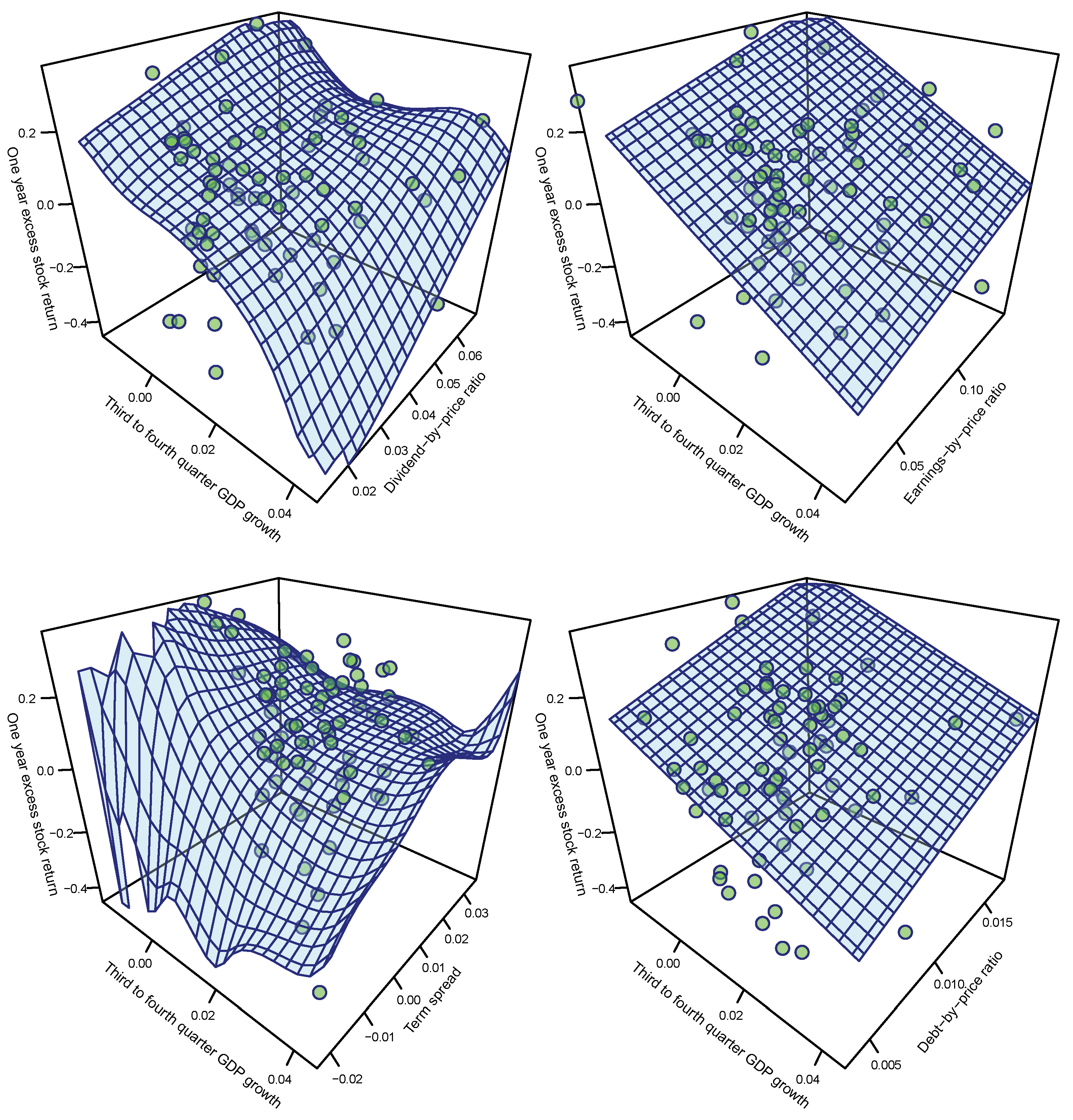As shown in Figure 2, the debt-by-price ratio signals more persistent business conditions, whereas the GDP growth signals shorter-term fluctuations. To get a better understanding, Figure 6 shows the relationship between the one year excess stock returns and the combination of third to fourth quarter GDP growth with dividend-by-price ratio, earnings-by-price ratio, term spread and debt-by-price ratio under the risk-free benchmark by the estimated nonparametric function $\widehat{m}$ (light blue surface) together with the underlying observations (green balls). It can be observed that a high debt-by-price ratio of 1.7% and a low third to fourth quarter GDP growth rate of −1.6% predict an extremely high one-year excess stock return of 39%.

5. Conclusions

In this paper, we extend the application of forecasting stock returns in Kyriakou et al. [35,36] in order to explore new predictive variables to beat the commonly discussed covariates in the literature. We predict one-year horizon stock returns in excess of the short-term rate, long-term rate, earnings-by-price ratio and inflation using the forecasting variables related to government debt and economic growth. A large number of covariates and their combinations have been examined for purposes of comparison throughout this research.

We propose a brand-new variable, debt-by-price ratio, which together with the third to fourth quarter economic growth prove to be extremely effective in the prediction of excess and nominal stock returns, individually and combined together. This superb performance outdoes the popular forecasting variables such as dividend-by-price ratio, earnings-by-price ratio, consumption–wealth-ratio, term spread and debt-by-GDP ratio by a perceptible difference, and is also valid under all the benchmarks; therefore, it can be used for various investment strategies including real value pension forecasts.

The overall conclusions are as follows. First, we find that US government debt and economic growth have a significant impact on stock prices. The most successful combination is debt-by-price ratio and third to fourth quarter GDP growth; using debt-by-price ratio or third to fourth quarter GDP growth as an individual predictor and two-dimensional predictors that include the third to fourth quarter GDP growth capture the best predictive performances. While the prediction of stock returns is incredibly puzzling, an appropriate choice of prediction model combined with suitable forecasting variables can achieve high-quality results. Second, this paper highlights the impact of liquidity on stock prices formulated in simple terms via government debt. There seems to be a political element of stock price variation that gives rise to worldwide distribution of wealth that is worth investigating further in the future. The limitation of the research includes lack of available data to expand the sample size and further study various predictive variables.

References

1. Binswanger, M. Stock market booms and real economic activity: Is this time different? Int. Rev. Econ. Financ. 2000, 9, 387–415. [Google Scholar] [CrossRef]
2. U.S. Office of Management and Budget and Federal Reserve Bank of St. Louis. Quarterly Total Public Debt as Percent of Gross Domestic Product. Available online: https://fred.stlouisfed.org/series/GFDEGDQ188S (accessed on 17 March 2020).
3. Antolin, P.; Schich, S.; Yermo, J. The economic impact of protracted low interest rates on pension funds and insurance companies. OECD J. Financ. Mark. Trends 2011, 2011, 237–256. [Google Scholar] [CrossRef]
4. Fama, E.F.; French, K.R. Business conditions and expected returns on stocks and bonds. J. Financ. Econ. 1989, 25, 23–49. [Google Scholar] [CrossRef]
5. Campbell, J.Y. A variance decomposition for stock returns. Econ. J. 1991, 101, 157–179. [Google Scholar] [CrossRef] [Green Version]
6. Campbell, J.Y. Stock returns and the term structure. J. Financ. Econ. 1987, 18, 373–399. [Google Scholar] [CrossRef] [Green Version]
7. Nelson, C.R. Inflation and rates of return on common stocks. J. Financ. 1976, 31, 471–483. [Google Scholar] [CrossRef]
8. Lettau, M.; Ludvigson, S. Consumption, aggregate wealth, and expected stock returns. J. Financ. 2001, 56, 815–849. [Google Scholar] [CrossRef] [Green Version]
9. Cochrane, J.H. Production-based asset pricing and the link between stock returns and economic fluctuations. J. Financ. 1991, 46, 209–237. [Google Scholar] [CrossRef]
10. Lamont, O.A. Investment plans and stock returns. J. Financ. 2000, 55, 2719–2745. [Google Scholar] [CrossRef]
11. Menzly, L.; Santos, T.; Veronesi, P. Understanding predictability. J. Political Econ. 2004, 112, 1–47. [Google Scholar] [CrossRef] [Green Version]
12. Piazzesi, M. Bond yields and the Federal Reserve. J. Political Econ. 2005, 113, 311–344. [Google Scholar] [CrossRef] [Green Version]
13. Cooper, I.; Priestley, R. Stock Return Predictability in a Production Economy; AFA 2006 Boston Meetings Paper; 2005. [Google Scholar] [CrossRef]
14. Møller, S.V.; Rangvid, J. End-of-the-year economic growth and time-varying expected returns. J. Financ. Econ. 2015, 115, 136–154. [Google Scholar] [CrossRef] [Green Version]
15. Lettau, M.; Ludvigson, S.C. Measuring and modeling variation in the risk-return trade-off. In Handbook of Financial Econometrics: Tools and Techniques; Elsevier: Amsterdam, The Netherlands, 2010; pp. 617–690. [Google Scholar]
16. U.S. Office of Management and Budget and Federal Reserve Bank of St. Louis. Annual Gross Federal Debt as Percent of Gross Domestic Product. Available online: https://fred.stlouisfed.org/series/GFDGDPA188S (accessed on 29 May 2021).
17. Rozeff, M.S. Dividend yields are equity risk premiums. J. Portf. Manag. 1984, 11, 68–75. [Google Scholar] [CrossRef]
18. Fama, E.F.; French, K.R. Dividend yields and expected stock returns. J. Financ. Econ. 1988, 22, 3–25. [Google Scholar] [CrossRef]
19. Campbell, J.Y.; Shiller, R.J. The dividend-price ratio and expectations of future dividends and discount factors. Rev. Financ. Stud. 1988, 1, 195–228. [Google Scholar] [CrossRef] [Green Version]
20. Campbell, J.Y.; Shiller, R.J. Stock prices, earnings, and expected dividends. J. Financ. 1988, 43, 661–676. [Google Scholar] [CrossRef]
21. Lamont, O. Earnings and expected returns. J. Financ. 1998, 53, 1563–1587. [Google Scholar] [CrossRef]
22. Rangvid, J. Output and expected returns. J. Financ. Econ. 2006, 81, 595–624. [Google Scholar] [CrossRef] [Green Version]
23. Croce, M.M.; Nguyen, T.T.; Raymond, S.; Schmid, L. Government debt and the returns to innovation. J. Financ. Econ. 2019, 132, 205–225. [Google Scholar] [CrossRef]
24. Elmendorf, D.W.; Mankiw, N.G. Government debt. Handb. Macroecon. 1999, 1, 1615–1669. [Google Scholar]
25. Modigliani, F. Long-run implications of alternative fiscal policies and the burden of the national debt. Econ. J. 1961, 71, 730–755. [Google Scholar] [CrossRef]
26. Kumar, M.M.S.; Baldacci, M.E. Fiscal Deficits, Public Debt, and Sovereign Bond Yields; Number 10-184; International Monetary Fund: Washington, DC USA, 2010. [Google Scholar]
27. Darrat, A.F. On fiscal policy and the stock market. J. Money Credit Bank. 1988, 20, 353–363. [Google Scholar] [CrossRef]
28. Darrat, A.F. Stock returns, money, and fiscal deficits. J. Financ. Quant. Anal. 1990, 25, 387–398. [Google Scholar] [CrossRef]
29. Darrat, A.F. The impact of federal debt upon stock prices in the United States. J. Post Keynes. Econ. 1990, 12, 375–389. [Google Scholar] [CrossRef]
30. Goyal, A.; Welch, I. A comprehensive look at the empirical performance of equity premium prediction. Rev. Financ. Stud. 2008, 21, 1455–1508. [Google Scholar]
31. Campbell, J.Y. Consumption-based asset pricing. Handb. Econ. Financ. 2003, 1, 803–887. [Google Scholar] [CrossRef] [Green Version]
32. Cochrane, J. Financial Markets and the Real Economy; Technical Report; National Bureau of Economic Research: Cambridge, MA, USA, 2005. [Google Scholar]
33. Rapach, D.; Zhou, G. Forecasting stock returns. In Handbook of Economic Forecasting; Elsevier: Amsterdam, The Netherlands, 2013; Volume 2, pp. 328–383. [Google Scholar]
34. Chang, C.L.; Ilomäki, J.; Laurila, H.; McAleer, M. Long run returns predictability and volatility with moving averages. Risks 2018, 6, 105. [Google Scholar] [CrossRef] [Green Version]
35. Kyriakou, I.; Mousavi, P.; Nielsen, J.P.; Scholz, M. Longer-Term Forecasting of Excess Stock Returns—The Five-Year Case. Mathematics 2020, 8, 927. [Google Scholar] [CrossRef]
36. Kyriakou, I.; Mousavi, P.; Nielsen, J.P.; Scholz, M. Forecasting benchmarks of long-term stock returns via machine learning. Ann. Oper. Res. 2021, 297, 221–240. [Google Scholar] [CrossRef] [Green Version]
37. Nielsen, J.; Sperlich, S. Prediction of stock returns: A new way to look at it. ASTIN Bull. 2003, 33, 399–417. [Google Scholar] [CrossRef] [Green Version]
38. Scholz, M.; Nielsen, J.; Sperlich, S. Nonparametric prediction of stock returns based on yearly data: The long-term view. Insur. Math. Econ. 2015, 65, 143–155. [Google Scholar] [CrossRef]
39. Scholz, M.; Sperlich, S.; Nielsen, J. Nonparametric long term prediction of stock returns with generated bond yields. Insur. Math. Econ. 2016, 69, 82–96. [Google Scholar] [CrossRef] [Green Version]
40. Mammen, E.; Nielsen, J.P.; Scholz, M.; Sperlich, S. Conditional variance forecasts for long-term stock returns. Risks 2019, 7, 113. [Google Scholar] [CrossRef] [Green Version]
41. Asimit, V.; Kyriakou, I.; Nielsen, J.P. Special Issue “Machine Learning in Insurance”. Risks 2020, 8, 54. [Google Scholar] [CrossRef]
42. Györfi, L.; Härdle, W.; Sarda, P.; Vieu, P. Nonparametric Curve Estimation from Time Series; Springer: Berlin/Heidelberg, Germany, 2013; Volume 60. [Google Scholar]
43. Gerrard, R.; Hiabu, M.; Nielsen, J.P.; Vodička, P. Long-term real dynamic investment planning. Insur. Math. Econ. 2020. [Google Scholar] [CrossRef]
44. U.S. Bureau of Economic Analysis. Gross Domestic Product and Consumer Spending Data. Available online: https://www.bea.gov/data (accessed on 17 March 2020).
45. U.S. Office of Management and Budget and Federal Reserve Bank of St. Louis. Industrial Production: Total Index. Available online: https://fred.stlouisfed.org/series/IPB50001SQ (accessed on 17 March 2020).
46. U.S. Department of the Treasury Bureau of the Fiscal Service Database. Public Debt Reports. Available online: https://www.treasurydirect.gov/govt/reports/pd/pd.htm (accessed on 17 March 2020).
47. Shiller, R. U.S. Stock Markets 1871-Present and CAPE Ratio. Available online: http://www.econ.yale.edu/~shiller/data.htm (accessed on 17 March 2020).
48. U.S. Office of Management and Budget and Federal Reserve Bank of St. Louis. 6-Month Treasury Bill: Secondary Market Rate. Available online: https://fred.stlouisfed.org/series/TB6MS (accessed on 17 March 2020).
49. Goyal, A. Consumption-Wealth Ratio Data. Available online: http://www.hec.unil.ch/agoyal (accessed on 17 March 2020).
50. National Bureau of Economic Research. Business Cycle Dating. Available online: https://www.nber.org/cycles.html (accessed on 17 March 2020).
51. Resnick, B.G.; Shoesmith, G.L. Using the yield curve to time the stock market. Financ. Anal. J. 2002, 58, 82–90. [Google Scholar] [CrossRef]
52. Campbell, J.Y.; Shiller, R.J. Cointegration and tests of present value models. J. Political Econ. 1987, 95, 1062–1088. [Google Scholar] [CrossRef] [Green Version]
53. Goyal, A.; Welch, I. Predicting the equity premium with dividend ratios. Manag. Sci. 2003, 49, 639–654. [Google Scholar] [CrossRef] [Green Version]
54. Ang, A.; Bekaert, G. How regimes affect asset allocation. Financ. Anal. J. 2004, 60, 86–99. [Google Scholar] [CrossRef]
55. Lettau, M.; Ludvigson, S.C. Expected returns and expected dividend growth. J. Financ. Econ. 2005, 76, 583–626. [Google Scholar] [CrossRef] [Green Version]
56. Klein, M.C.; Pettis, M. Trade Wars Are Class Wars: How Rising Inequality Distorts the Global Economy and Threatens International Peace; Yale University Press: New Haven, CT, USA, 2020. [Google Scholar]
57. Jagannathan, R.; Wang, Y. Lazy investors, discretionary consumption, and the cross-section of stock returns. J. Financ. 2007, 62, 1623–1661. [Google Scholar] [CrossRef] [Green Version]
58. Ritter, J.R.; Chopra, N. Portfolio rebalancing and the turn-of-the-year effect. J. Financ. 1989, 44, 149–166. [Google Scholar] [CrossRef]
59. He, J.; Ng, L.; Wang, Q. Quarterly trading patterns of financial institutions. J. Bus. 2004, 77, 493–509. [Google Scholar] [CrossRef]
60. Abel, A.B.; Eberly, J.C.; Panageas, S. Optimal inattention to the stock market with information costs and transactions costs. Econometrica 2013, 81, 1455–1481. [Google Scholar]
61. Wen, Y. The business cycle effects of Christmas. J. Monet. Econ. 2002, 49, 1289–1314. [Google Scholar] [CrossRef]
62. Campbell, J.Y.; Cochrane, J.H. By force of habit: A consumption-based explanation of aggregate stock market behavior. J. Political Econ. 1999, 107, 205–251. [Google Scholar] [CrossRef]
Figure 1. The United States annual debt-to-GDP ratio % growth (dark blue line), calculated using the annual gross federal debt as percent of gross domestic product [16]. The sample period is 1947–2020.
Mathematics 09 01550 g001
Figure 2. The most successful forecasting variables detected in this analysis (dark blue line). From top to bottom: debt-by-price ratio, third to fourth quarter GDP growth and term spread. Vertical lines (gray area) are the NBER business-cycles (recessions). The sample period is 1947–2020.
Mathematics 09 01550 g002
Figure 3. Risk-free benchmark. Relation between excess stock returns and debt-by-price ratio. Estimated nonparametric function m ^ (dark blue line), linear model (dotted red line), observations (green balls). The sample period is 1947–2020.
Mathematics 09 01550 g003
Figure 4. Risk-free benchmark. Relation between excess stock returns and third to fourth quarter GDP growth. Estimated nonparametric function m ^ (dark blue line), linear model (dotted red line), observations (green balls). The sample period is 1947–2020.
Mathematics 09 01550 g004
Figure 5. Risk-free benchmark. Relation between excess stock returns and term spread. Estimated nonparametric function m ^ (dark blue line), linear model (dotted red line), observations (green balls). The sample period is 1947–2020.
Mathematics 09 01550 g005
Figure 6. Risk-free rate benchmark. Relation between one year excess stock returns and the combination of third to fourth quarter GDP growth with the dividend-by-price ratio, earnings-by-price ratio, term spread and the debt-by-price ratio. Estimated nonparametric function m ^ (light blue surface), observations (green balls). The sample period is 1947–2020.
Mathematics 09 01550 g006