A Review of Spatiotemporal Models for Count Data in R Packages. A Case Study of COVID-19 Data

Abstract

Spatiotemporal models for count data are required in a wide range of scientific fields, and they have become particularly crucial today because of their ability to analyze COVID-19-related data. The main objective of this paper is to present a review describing the most important approaches, and we monitor their performance under the same dataset. For this review, we focus on the three R-packages that can be used for this purpose, and the different models assessed are representative of the two most widespread methodologies used to analyze spatiotemporal count data: the classical approach and the Bayesian point of view. A COVID-19-related case study is analyzed as an illustration of these different methodologies. Because of the current urgent need for monitoring and predicting data in the COVID-19 pandemic, this case study is, in itself, of particular importance and can be considered the secondary objective of this work. Satisfactory and promising results have been obtained in this second goal. With respect to the main objective, it has been seen that, although the three models provide similar results in our case study, their different properties and flexibility allow us to choose the model depending on the application at hand.

1. Introduction

Spatiotemporal models for count data relate to problems where the variable of interes take non-negative integer values, and these integers arise from counting occurrences of an event in a geographic areal unit in a certain time unit. The observations refer to a set of contiguous non-overlapping areal units for consecutive time periods. Additionally, a series of covariates are measured for each unit of area and time; these covariates could be common in time or area, and they can be discrete, continuous, or even factors.

These models are needed in a variety of settings: agricultural production [1], fishing catches [2], volcano eruptions [3], crime counts [4], cases of pulmonary disease [5], etc. The reasons for modeling these data are diverse and can range from estimating the effect of a risk factor to a response, identify clusters of adjacent areas with similar response patterns, or forecasting future observations. Different modeling strategies have been proposed to deal with this array of scenarios comprising spatiotemporal data. The strategies become more complex when the aim is to build multivariate spatiotemporal models for the joint analysis of different variables that include specific and shared spatial and temporal effects [6].

This kind of data presents two major challenges with respect to classical linear regression models. Firstly, it is well known that the normal assumption is not appropriate for count data modeling, and generalized linear models with Poisson, binomial, or negative binomial distributions must be used [7]. Secondly, spatiotemporal autocorrelation, i.e., that observations from geographically close areal units and temporally close time periods tend to have more similar values than units and time periods that are further apart, results in complicated correlation structures, and, as a result, parameter estimation is not straightforward and different approaches have been developed for this purpose [8,9]. Due to the diversity of applications, data types, and conceptual approaches, there is a broad range of literature on spatiotemporal modeling. Two excellent books that provide a gradual entry to the methodological aspects of spatiotemporal statistics and outline some of the standard techniques used in this area are References [10,11]. An overview of different spatiotemporal modeling approaches can also be found in Reference [12].

Since December 2019, when the first cases of the illness caused by the coronavirus SARS-CoV-2 were reported in Wuhan, China, the SARS-CoV-2 virus has spread world-wide. According to the website of the World Head Organization (WHO) [13], the virus has caused more than 127 million infections and 2.78 million deaths around the world as of 30 March 2021, and it is currently impossible to predict how many people will be affected by it. An effective way to control the spread of the infection is to understand and predict key epidemiological data. Epidemic models have provided powerful insight to study data about the coronavirus pandemic, including the number of new cases and deaths in a given area over time. Epidemic models to study the spread of infectious diseases date back to the beginning of the twentieth century. The susceptible-infected-recovered (SIR) models developed by Kermack and McKendrick [14] were the first mathematical models developed to study the transmission dynamics of infectious diseases. The SIR and SEIR (Susceptible, Exposed, Infectious, and Removed) models have been improved and used for analyzing and characterizing the COVID-19 epidemic [15,16,17], as well, in Spain [18,19,20]. In addition to the crucial role played by the above described epidemic models, other models are also being adapted to examine different aspects of the COVID-19 pandemic [21,22]. In particular, mathematical modeling of patient hospitalization is essential, as it may help raise awareness of a possible collapse of the health-care systems due to an increase in the number of patients needing hospitalization. Therefore, robust prediction models are vital to support decisions on population and community-level interventions to control the spread of the virus and to prevent the collapse of health services. Models for this type of data are rather different from epidemic models because the prediction of hospitalizations requires previously obtained COVID-19 data, such as the number of people tested and/or infected or the population at risk. Additionally, models relating to the number of hospitalizations have to manage observations over time in several geographical areas, such as health departments. Each temporal observation relates to an areal unit and, in this case, refers to count measures for the unit: number of COVID-19 hospitalizations in an areal unit per day. Moreover, given the contribution of people’s mobility to the spread of the virus, these models should be able to adjust for people’s mobility between neighboring health areas.

The main purpose of the current study is to present a review describing three different approaches that can be used to model and analyze spatiotemporal count data. In particular, we revisit three different type of models that are representative of the two most widespread methodologies used to analyze this type of data. The first two models are formulated following the classical statistical paradigm and the last one follows the Bayesian point of view (see Reference [23] for a survey of the hierarchical Bayesian approach and Reference [24] for Bayesian disease mapping). Of the two classical approaches, one is based on Penalized Likelihood and the other on Estimating Equations [25].

For this review, we focus on the three R-packages that can be used for this purpose. These packages are: the surveillance package [26]—the model implemented in this package is based on a likelihood model, working on the classical methodology; the Mcglm package [27], whose model is based on estimating equations, working on the classical methodology; and, finally, the CARBayesST package [28], based on the Bayesian methodology. The main properties and characteristics of each of them will be discussed. This can be useful as a guide for scientists in different experimental fields.

Other approaches include Dynamic Spatial Panel Data models [29,30] that are more usual in the econometric literature; Machine-Learning techniques, such as Classification and Regression Trees, Support Vector Machine, and Multilayer perceptron Neural Network [31]. Generalized Additive Models have also been used in applied real problems with spatiotemporal data [32,33,34]. With respect to Bayesian models, different types of spatial, temporal, and spatiotemporal random effects, not included in the CARBayesST package, can also be used, such as non-parametric estimation of trends [35] or splines [36,37]. The secondary, but also important, goal of this paper is to apply the reviewed models and compare their performance in the prediction of the number of COVID-19 hospitalizations given the number of infected people in the 24 health departments of the Valencian Community, Spain. The Valencian community is the fourth most populous autonomous community of Spain. It is a rich region with very high residential density along the coast and a lot of tourism and significant exports. Concern about the evolution of the pandemic in this community led the regional presidency to ask the scientific community for advice about some decision-making regarding the pandemic. Our results will be very useful for this aim.

The article is organized as follows: In Section 2, a descriptive analysis of the data is performed, followed by the mathematical details of the three models. Then, the three models are applied to COVID-19 data in Section 3. Our results are discussed in Section 4, and, finally, the conclusions are stated in Section 5.

A simulated dataset and code in R for illustrating the implementation of the different approaches are available at http://www3.uji.es/~mibanez/MDPIcode (accessed on 1 June 2021).

2. Methodology

In this section, we describe the spatiotemporal approaches to predict the number of COVID-19 hospitalizations. We begin by describing the data sources, and then we describe the analytic models and fitting processes.

2.1. The COVID-19 Dataset: Description and Cleasing

The dataset is comprised of the number of daily new positive cases of COVID-19 (tested via PCR (polymerase chain reaction) or the antigen test) and the daily number of hospital admissions due to COVID-19 (daily hospitalizations) in the Valencian Community, a large area of Eastern Spain (from 28 June 2020 to 13 December 2020). This area is organized into $K=24$ different health departments, and the dataset is comprised of both temporal series (hospitalized/new positive cases) for all departments. Figure 1 shows the spatial location of the Valencian Community within Spain and its division into 24 health departments and the distribution of the population (×100,000 people) in these 24 health departments. As can be observed, the population size in the health departments is very heterogeneous.

The number of new daily positive cases by health department is published regularly on an open data platform of the Generalitat Valenciana (Valencian regional goverment) [38], and the number of daily hospitalizations (by health department) has been provided by the “Data Science for COVID-19 TaskForce” group of the Valencian Community, with the commitment not to show detailed maps or identifiable information about this variable, which is public only at the aggregated level of the entire Valencian Community. As an illustration, eight of the 24 health departments have been anonymized and will be used to illustrate all the steps in the different analyses. However, the models are fitted using the data of the 24 health departments, and the estimations of the parameters and the goodness of fit measures shown in the paper are related to all of them.

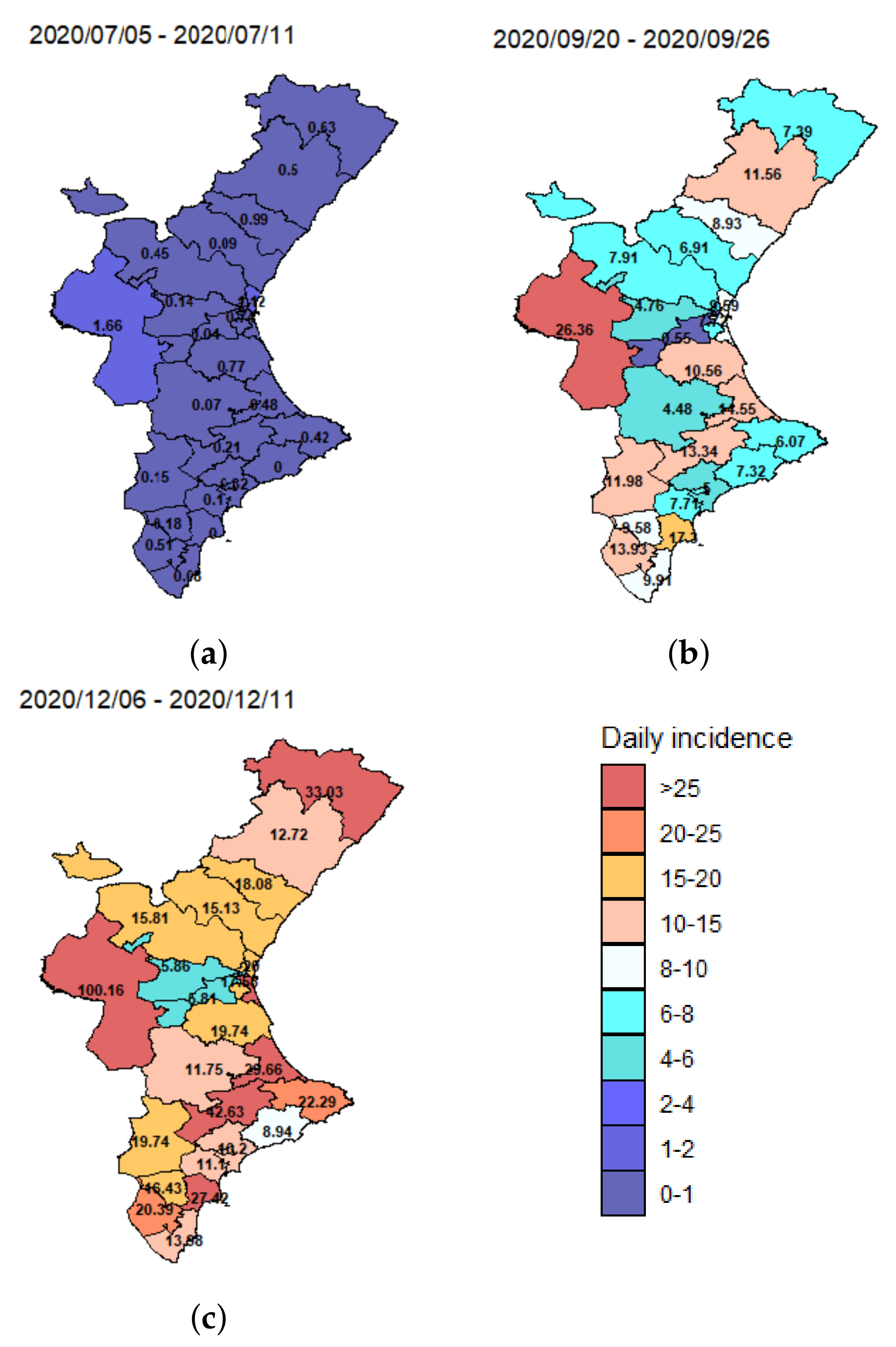
Although these data may be subject to temporal biases due to changing testing regimes, among other problems, the mean spatial incidence (number of new cases divided by population size) for three different weeks (5–11 July 2020, 20–26 September 2020 and 4–11 December 2020) plotted in Figure 2, shows strong variation across the different health departments over time.

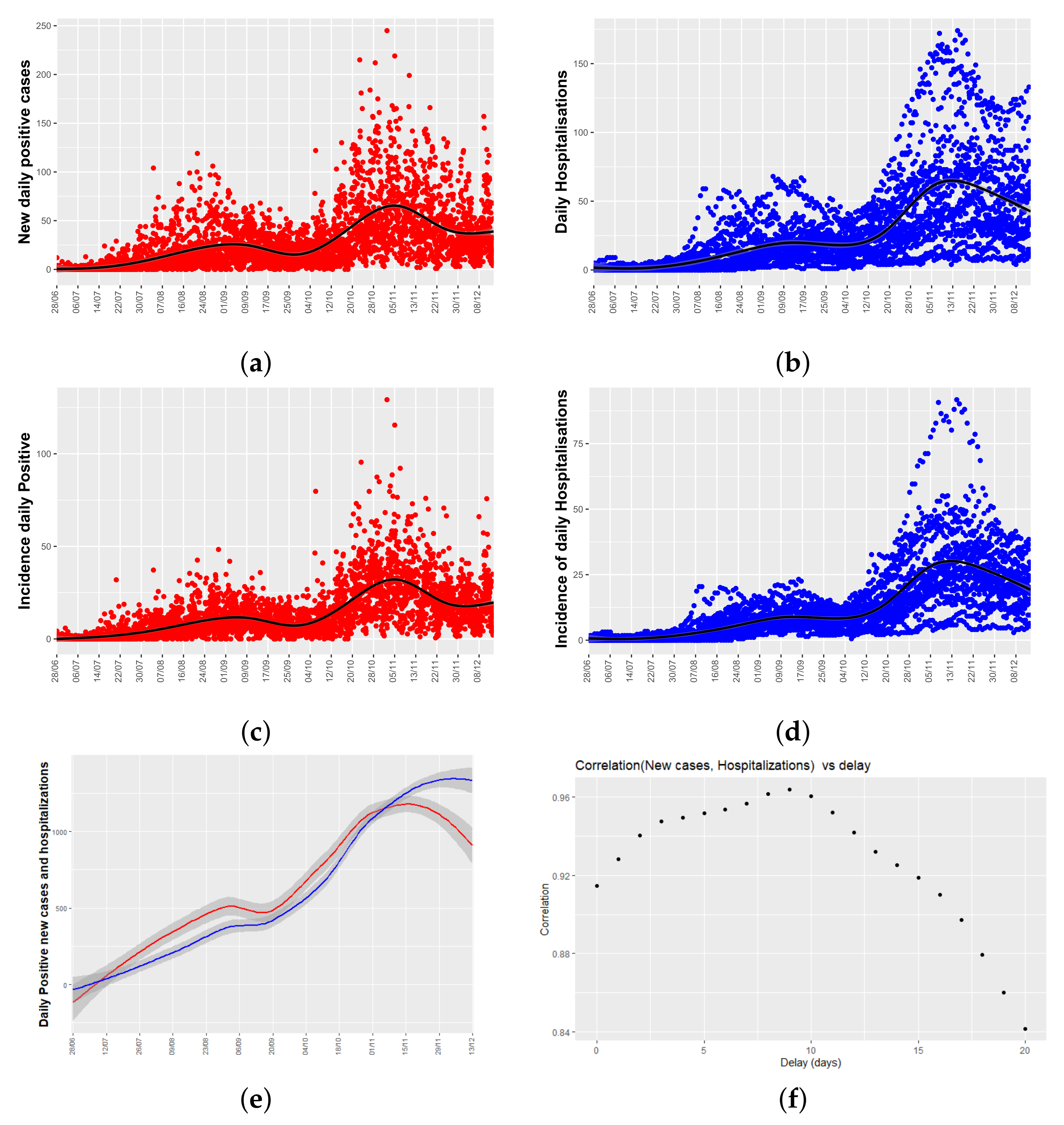
Figure 3a,b show time series plots for both variables of interest: the number of daily new positive cases and the number of daily hospitalizations per health department. From now on, daily hospitalizations will mean the total number of people admitted to hospital due to COVID-19 each day. Figure 3a shows a peak of new cases in late August, and another in mid-November, two and a half months apart, and the same temporal pattern appears in the series of hospitalizations.

As different health department have different population sizes, Figure 3c,d show the relative data, and it is said, the number of new positive cases, and daily hospitalizations corrected by the population size of each health department (incidence values). As can be seen, temporal patters remain unchanged. Figure 3e shows a lowess smoothing of the total number of new positive cases and hospitalizations per day (adding the values of the 24 health departments). From Figure 3e, it can be seen that there is a time lag between both time series.

As a first approach to analyze the delay between both time series, a cross-correlogram (see Figure 3f) has been used. It plots a measure of correlation of both time series as a function of the displacement (days) of daily positives relative to the daily hospitalizations. In our case, we have used the Pearson correlation coefficient that is a standard descriptive measure of the linear correlation between two quantitative variables. Figure 3f shows that the coefficients are close to 1 for any time lag, indicating high linear correlation between daily hospitalizations and incidence, and that there are two local maximums at the time lag of 9 and 5 days. These values will be used in Section 3.

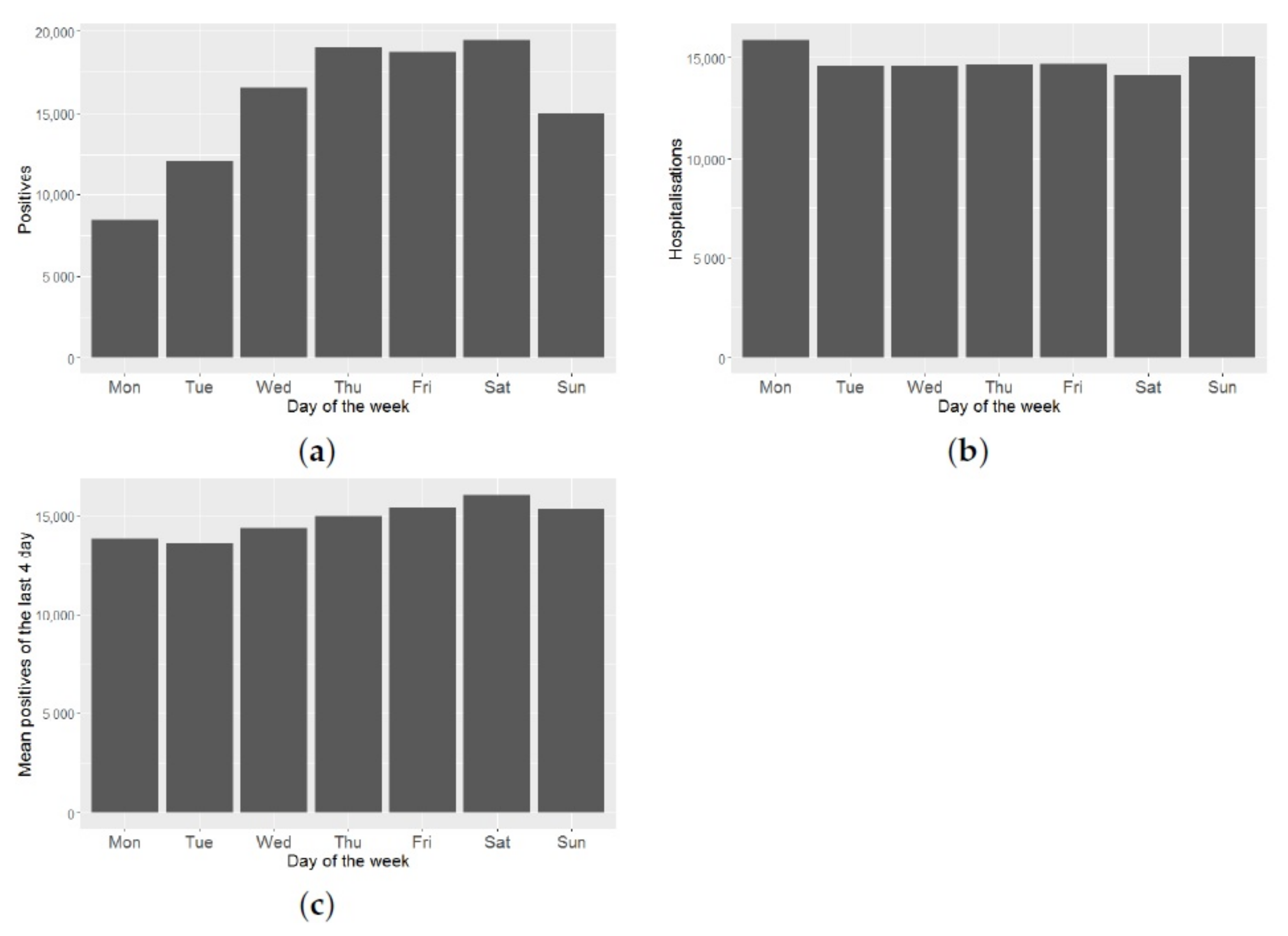
These data may be subject to temporal biases due to under-reporting on weekends and/or on non-working days. Figure 4a shows a great variability in the number of positives, depending on the day of the week. As can be seen in Figure 4b, this effect does not hold for the number of daily hospitalizations. Therefore, this effect is an artefact, due to when the official data is reported. To minimize this reporting bias, we smooth the time series of daily positives, taking the average of each datum and its three predecessors. By doing this smoothing, we reduce this effect, as can be seen from Figure 4c.

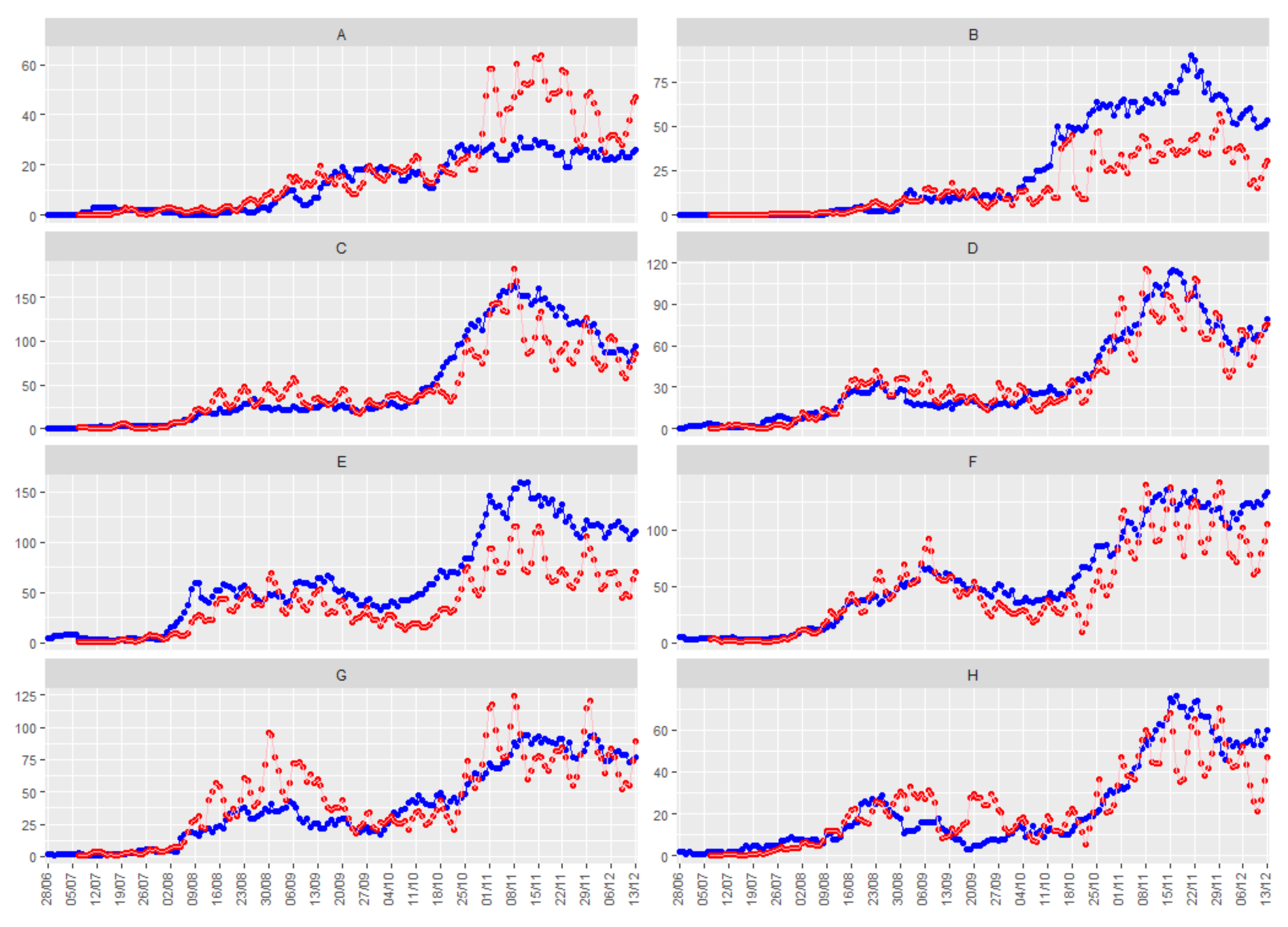
Finally, both effects are corrected. Figure 5 shows the smoothed number of positive daily cases (in red), together with the number of people hospitalized due to COVID-19 (in blue) for the eight illustrative health departments, with a time delay of 9 days between both series.

To conclude, when looking for the best model, we explored the relationship between the mean and the variance of the hospitalization data collected at each instant of time. We have seen that there is a potential relationship between mean and variance. This relationship is crucial for the modeling, as will be seen in the following sections.

2.2. Models

Throughout this section, $Y_{kt}$ will denote the observation taken in the k-th areal unit $S_k$ at time t, for $k=1,\dots ,K$ and $t=1,\cdots ,N$. Then, ${\mathbf{Y}}_t=(Y_{1t},\dots ,Y_{Kt})$, ($t=1,\dots ,N$), will be a spatiotemporal count series, i.e., count data recorded in the areal units for consecutive discrete time periods. We assume that we also have space-time varying covariates ${\mathbf{X}}_t=(X_{1t},\dots ,X_{Kt})$ recorded at the same times and locations. Our main objective will be to predict future observations of the spatiotemporal time series ${\mathbf{Y}}_t$, by taking into account the spatiotemporal covariates ${\mathbf{X}}_t$ and the spatial and temporal relationships between the observations.

2.2.1. Endemic-Epidemic Models. R Package Surveillance

Endemic-epidemic (EE) models are a class of statistical time series models for multivariate surveillance counts proposed by Ref. [39] and extended in Refs. [26,40,41]).

In its current formulation and implementation in the R package surveillance [26], the EE framework uses incidence from the preceding week, $t-1$, to explain the incidence in week t. So, the counts, $Y_{kt}|{\mathbf{Y}}_{t-1}$, are assumed to be Poisson or Negative Binomial distributed with the conditional mean:

$${\mu }_{kt}=e_{kt}{\nu }_{kt}+{\lambda }_{kt}{Y}_{k,t-1}+{\varphi }_{kt}\sum _{q\ne k}{w}_{qk}{Y}_{q,t-1},{\nu }_{kt},{\lambda }_{kt},{\varphi }_{kt}>0,$$

(1)

and overdispersion parameter, in the Negative Binomial case, ${\psi }_k>0$.

The first term of the summation is called the endemic component and can cover exogenous factors, such as temporal trends, seasonality, sociodemographics, and/or population. The second term of the summation, that models the effect of the previous values of the response variable in time, is usually denoted as the ’autoregressive’ component, whereas the last term, called ’spatiotemporal component, describes how the response variable in region k is linked to previous cases in the same and adjacent regions. These two terms constitute the epidemic component of the model.

The parameters ${\nu }_{kt}$, ${\lambda }_{kt}$, and ${\varphi }_{kt}$ are constrained to be non-negative and can be modeled by allowing for log-linear predictors in all three components, as sine-cosine terms to account for seasonality [42], long-term temporal trends, or/and covariates [43,44].

$$\begin{array}{ccc}\hfill log({\nu }_{kt})& =& {\alpha }^{(\nu )}+b_k^{(\nu )}+{\beta }^{(\nu )}{z}_{kt}^{(\nu )}\hfill \\ \hfill log({\lambda }_{kt})& =& {\alpha }^{(\lambda )}+b_k^{(\lambda )}+{\beta }^{(\lambda )}{z}_{kt}^{(\lambda )}\hfill \\ \hfill log({\varphi }_{kt})& =& {\alpha }^{(\varphi )}+b_k^{(\varphi )}+{\beta }^{(\varphi )}{z}_{kt}^{(\varphi )}.\hfill \end{array}$$

(2)

This form allows for fixed intercepts ${\alpha }^{(.)}$, region-specific intercepts $b_k^{(.)}$ and exogenous covariates $z_{kt}^{(.)}$ in each model compartment. Population fraction, population density, border effects, etc., can be used as covariates. The region-specific intercepts, $b_k^{(.)}$, can be treated as fixed effects or as random effects accounting for heterogeneity between the regions. When they are treated as random effects, they are assumed to be independent and identically distributed across k, but can be correlated across the model components, following a Gaussian distribution:

$$\begin{array}{c}\hfill b_k:=(b_k^{(\nu )},b_k^{(\lambda )},b_k^{(\varphi )})\sim N((0,0,0),{\Sigma }_b).\end{array}$$

We will see this part in more detail in Section 3.1.

Maximum likelihood (ML) estimates are obtained using penalized likelihood approaches.

This basic model has been extended to cover other different aspects of disease modeling (see Reference [22] for references). Recent extensions include methodology to adjust for under-reporting [22,45] or to allow different lags in the auto-regressive part of the model (package hhh4addon [46,47]), modeling the conditional mean $Y_{kt}|{\mathbf{Y}}_{t-1},\cdots {\mathbf{Y}}_{t-D}$ as:

$${\mu }_{kt}=e_{kt}{\nu }_{kt}+{\lambda }_k\sum _q\sum _{d=1}^D{w}_{qk}{Y}_{q,t-d},{\nu }_{kt},{\lambda }_k>0,$$

(3)

where D is the maximum lag considered.

In Reference [48], the authors extend the basic endemic-epidemic spatiotemporal model to fit multivariate time series of counts $y_{gkt}$ stratified by (age) groups, in addition to spatial regions. Therefore, they define a contact matrix $C=(c_{g^{\prime }g})$, where $c_{g^{\prime }g}\ge 0$ quantifies the average number of contacts of an individual of group $g^{\prime }$ with individuals of group g, and the spatiotemporal model is now modeled as:

$${\mu }_{gkt}=e_{gkt}{\nu }_{gkt}+{\lambda }_{gkt}\sum _{g^{\prime }q}{c}_{g^{\prime }g}{w}_{qk}{Y}_{g^{\prime },q,t-1},{\nu }_{kt},{\lambda }_k>0,$$

(4)

where both the endemic and epidemic predictors may gain group-specific effects. This model is implemented in the R-package hhh4contacts [49].

Forecast

The surveillance package uses the function hhh4() to fit the models and implements the oneStepAhead() function, which computes successive one-step-ahead predictions for the fitted model, also providing confident intervals for the predictions and plot methods.

A discussion of suitable measures to evaluate the quality of a point forecast can be found in Reference [50] and several scoring rules based on the one-step-ahead predictions [40] are implemented in the function scores(), although we will consider the root mean squared error of the predictions (RMSEp). Another function implemented in the package related to the oneStepAhead() function is the calibrationTest() function, which implements calibration tests for Poisson or Negative Binomial predictions of count data based on proper scoring rules; it is described in detail in Reference [51].

Long-term predictions do not have much sense in our context because we do not know the long-term evolution of the covariates.

2.2.2. Multivariate Covariance Generalized Linear Models. R Package Mcglm

Under the same previous assumption of predicting ${\mathbf{Y}}_t=(Y_{1t},\dots ,Y_{Kt})$ in terms of spatiotemporal correlations and ${\mathbf{X}}_t=(X_{1t},\dots ,X_{Kt})$ covariates, we can use the multivariate covariance generalized linear model (McGLM) introduced in Reference [52]. This model is a general and flexible statistical model to deal with multivariate count data that explicitly models the marginal covariance matrix combining a covariance link function and a matrix linear predictor composed of known matrices.

Let ${\mathbf{Y}}_{K\times N}=\{{\mathbf{Y}}_1,\cdots ,{\mathbf{Y}}_N\}$ be the outcome matrix, and let $M_{K\times N}=\{{\mu }_1,\cdots ,{\mu }_N\}$ denote the corresponding matrix of expected values.

The McGLM as proposed by Reference [52] is given by

$$\begin{array}{ccc}\hfill E(\mathbf{Y})& =& ({\mu }_1,\cdots ,{\mu }_N)=(g_1^{-1}(X_1{\beta }_1),...,g_N^{-1}(X_N{\beta }_N))\hfill \end{array}$$

(5)

$$\begin{array}{ccc}\hfill Var(\mathbf{Y})& =& C={\Sigma }_t\underset{G}{⨂}{\Sigma }_b,\hfill \end{array}$$

(6)

where $g_t$ are monotonic differentiable link functions, $X_t$ denotes an $K\times k_t$ design matrix, ${\beta }_t$ is a regression parameter vector to be estimated, ${\Sigma }_t$ is the $K\times K$ covariance matrix within the response variable $Y_t$ for $t=1,\cdots ,N$, ${\Sigma }_b$ the $N\times N$ correlation matrix whose components denote the correlation between outcomes, and

$$\begin{array}{c}\hfill {\Sigma }_N\underset{G}{⨂}{\Sigma }_b=Bdiag({\tilde{\Sigma }}_1,\cdots ,{\tilde{\Sigma }}_N)({\Sigma }_b⨂I)Bdiag({\tilde{\Sigma }}_1^{-T},\cdots ,{\tilde{\Sigma }}_N^{-T})\end{array}$$

is the generalized Kronecker product [53]. The matrix ${\tilde{\Sigma }}_t$ denotes the lower triangular matrix of the Cholesky decomposition of ${\Sigma }_t$. The operator $Bdiag$ denotes a block diagonal matrix, and I denotes a $K\times K$ identity matrix.

Following Reference [52], ${\Sigma }_t$, the covariance matrix within outcomes can be defined as:

$$\begin{array}{c}\hfill {\Sigma }_t=V{({\mu }_t;p_t)}^{\frac{1}{2}}(\Omega ({\tau }_t))V{({\mu }_t;p_t)}^{\frac{1}{2}}.\end{array}$$

(7)

And a common and very flexible choice for $V({\mu }_t;p_t)$ in the case of modeling count data, is the Poisson-Tweedie dispersion function [54]:

$$\begin{array}{c}\hfill V({\mu }_t;p_t)=diag({\mu }_t^{p_t}),\end{array}$$

(8)

that is a diagonal matrix whose main entries are given by the power variance function. Particular cases of the Poisson-Tweedie family of distributions are the Hermite (p = 0), Neyman Type A (p = 1), Negative Binomial (p = 2), and Poisson-inverse Gaussian (p = 3) distributions.

In Equation (7), the dispersion matrix $\Omega ({\tau }_t)$ describes the part of the covariance within outcomes that does not depend on the mean structure. Jorgensen et al. [54], among others, propose to model it using a matrix linear predictor combined with a covariance link function, i.e.,

$$h(\Omega ({\tau }_t))={\tau }_{t0}{Z}_{t0}+\cdots +{\tau }_{tD}{Z}_{tD},$$

(9)

where h is the covariance link function, $Z_{td}$ with $d=0,\cdots ,D$ are known matrices reflecting the covariance structure within the response variable $Y_t$, and ${\tau }_r=({\tau }_{r0},\cdots ,{\tau }_{rD})$ is a $(D+1)\times 1$ vector of dispersion parameters.

McGLMs are fitted based on the estimating function approach described in detail by References [52,55]. A general overview of the algorithm and the asymptotic distribution of the estimating function estimators can be found in Reference [27]. As a method for selecting the components of the matrix linear predictor (variable selection), the score information criterion (SIC) is proposed. This is an important tool to assist with the selection of the linear and matrix linear predictor components, but, unfortunately, it is less useful for comparing models fitted using different link, variance, or covariance functions. The mcglm package implements the SIC to select the linear and matrix linear predictor components, with the mc_sic and mc_sic_covariance functions. To compare the goodness of non-nested models, the gof function provides the pseudo Akaike information criterion (pAIC), the pseudo Bayesian information criterion (pBIC), and the pseudo Kullback-Leibler information criterion (pKLIC).

Forecasting

Unfortunately, the mcglm package does not have any function implemented to predict future observations. However, once the model has been estimated, the mc link function can be used to approach the predictions. This function returns the inverse of the link function applied to the linear predictor, i.e., $\mu =g^{-1}(X\beta )$, as an approximation of the predictions sought.

2.2.3. Bayesian Hierarchical Generalized Linear Models. Carst Package

A great variety of spatiotemporal models for count data using generalized linear models (GLM) can be found in the Bayesian literature. To model these data a hierarchical model with spatiotemporal structured prior distributions is used. The spatiotemporal structure is modeled via sets of autocorrelated random effects with conditional autoregressive prior distributions and its spatiotemporal extensions. An excellent review can be found in Reference [28].

These methods have had a remarkable development, especially in disease mapping, thanks to the availability of estimation methods based on Monte Carlo Markov Chain. With respect to the software packages for implementing these models, although a great quantity of software packages can be found for implementing purely spatial models, such as BUGS [56] and R-INLA [57], software for spatiotemporal modeling is much less well developed and mainly focuses on geostatistical data. This was the motivation for developing the CARBayesST R package [28]. This package can fit several models for count data with different spatiotemporal structures. A useful tutorial is provided by Reference [58]. CARBayesST package has been recently used to study the case-fatality risk by COVID-19 in Colombia [59]. The general Bayesian hierarchical model for spatiotemporal count data is as follows:

$$\begin{array}{ccc}\hfill Y_{kt}& \sim & f(y_{kt}|{\mu }_{kt},\nu )\hfill \end{array}$$

(10)

$$\begin{array}{ccc}\hfill g({\mu }_{kt})& =& X_{kt}\beta +{\psi }_{kt}\hfill \end{array}$$

(11)

$$\begin{array}{ccc}\hfill \beta & \sim & N({\mu }_{\alpha },{\Sigma }_{\beta }).\hfill \end{array}$$

(12)

The probability function f is in the exponential family (not necessarily a Gaussian distribution), $\beta$ is the vector of covariate regression parameters, and a multivariate Gaussian prior is assumed. g can be any monotonic differentiable link function, and ${\psi }_{kt}$ is a latent component for areal unit k and time period t encompassing one or more sets of spatiotemporally autocorrelated random effects, we denote ${\psi }_t=({\psi }_{1t},\dots ,{\psi }_{Kt})$.

In this paper, we are just focusing on the models implemented in the CARBayesST package. In this package, binomial, Gaussian and Poisson data models can be used for the first level of the model, f in Equation (10), and different spatiotemporal structures for ${\psi }_{kt}$ in Equation () are given.

All models implemented in this package use random effects to introduce spatial autocorrelation into the response variable. For this purpose, CAR-type prior distributions and their space-time extensions are used. Spatial autocorrelation is induced via a non-negative symmetric matrix of adjacency $W=(w_{kj})$, where $w_{kj}$ represents the spatial closeness between units $(S_k,S_j)$. Larger valued elements represent spatial closeness between the two areas in question and spatially autocorrelated random effects, whereas zero values correspond to areas that are not spatially close and conditionally independent random effects given the remaining.

The models are outlined in

Table 1. Summary of the models available in the CARBayesST package.

ST.CARlinear [60]	Spatially varying linear time trends model
ST.CARanova [35]	Spatial and temporal autoregressive main
	effects and independent interaction model
ST.CARsepspatial [61]	Common temporal trend but varying spatial surfaces model
ST.CARar [62]	Spatially autocorrelated autoregressive of order 1 time series model
ST.CARadaptive [63]	Spatially adaptive smoothing model for localized spatial smoothing
ST.CARlocalized [64]	Spatiotemporal clustering model

[28]. In all cases, inference is based on Markov chain Monte Carlo (MCMC) simulation.

Forecasting

In order to predict future observations of the response variable, simulations from the posterior predictive distribution (the distribution of possible unobserved values conditional on the observed values) have to be obtained.

This predictive density can be approximated by Monte Carlo integration. If we denote the vector with all the parameters of the model by $\theta$:

$$f({\mathbf{Y}}_{N+h}|({\mathbf{Y}}_1,\dots ,{\mathbf{Y}}_N))\approx \frac{1}{n}\sum _j^{n}f({\hat{\mathbf{Y}}}_{N+h}|{\theta }^{(j)},({\mathbf{Y}}_1,\dots ,{\mathbf{Y}}_N)).$$

If a representative value is wanted, the mean of the predictive density can be obtained by taking into account the property that $E_{\theta }E({\mathbf{Y}}_{N+h}\mid \theta ))$ and approximating the mean again with respect to $\theta$:

$$E({\mathbf{Y}}_{N+h}|({\mathbf{Y}}_1,\dots ,{\mathbf{Y}}_N))=\frac{1}{n}\sum _j^{n}E({\mathbf{Y}}_{N+h}|{\theta }^{(j)},({\mathbf{Y}}_1,\dots ,{\mathbf{Y}}_N)).$$

Unfortunately, the CARBayesST package does not have any function implemented to predict future observations. For h = 1, it can be easily implemented using the samples of the posterior distributions of the parameters. For $h>1$, the simulation of the posterior distribution of the random effects should be implemented. In this case, for users who are not experts in R programming, just an approximation can be obtained, approximating the value of the random effect by the that of the previous prediction. This approximation will be used in Section 3.3.

In regard to credible intervals for the predictions, the CARBasyesST package provides the samples of the posterior distribution of the adjusted data and credible intervals for the fitted values can be easily obtained. Unfortunately, the calculus of credible intervals for forecasts would need again the simulation of the posterior distribution that it is not provided by the package.

3. Application

In this section, we particularize the general models reviewed in Section 2.2 and then we apply them to the COVID-19 data described in Section 2.1. We continue with the notation introduced in the previous section.

Since our primary goal is forecasting, the mean squared errors of the predictions (RMSEp) up to a five-day horizon are calculated. This is a classical approach to measure their performance. Therefore, data from 28 June 2020 to 8 December 2020 are used to fit the different models. The root mean square error comparing observed and fitted values (RMSEf) are computed in all cases to describe the goodness the fits. Data from 9 to 13 of December 2020, jointly with the five-day horizon forecasts of each model, are used to compute the root mean square error of the predictions (RMSEp). If we want to use real data of positive cases, the horizon of prediction is limited, but taking a horizon of five is considered enough, within our possibilities, to prevent the collapse of hospitals.

Each model is adjusted using the corresponding statistical methodology included in its corresponding R package. Additional specific measures of goodness of fit are given; these other measures will be useful to compare different models within the same R package.

3.1. Endemic-Epidemic Models

As stated in Section 2.2.1, let us consider that the counts of daily hospitalizations in the k-th health department, on the t-th day, $Y_{kt}$, follows a Poisson distribution with mean as in Equation (1).

If $p_k$ denotes the population of the k-th health department, we assume in Equation (1) known population fractions

$$\begin{array}{c}\hfill e_{kt}=e_k=\frac{p_k}{{\sum }_{k=1}^{24}{p}_k},\forall t,\end{array}$$

and that $w_{qk}=I(q\sim k)$, i.e., $w_{qk}=1$ if both health areas have a common geographic border (assuming the epidemic only arrives from adjacent health areas), and 0 otherwise. Weights $w_{qk}=\frac{w_{qk}}{{\sum }_q{w}_{qk}}$ are normalized and restricted to be positive.

Covariates, such as number of positive cases, can be added to the model in different ways [26,65]. The simplest way is to include the covariates $x_{kt}$ in the formulation in the endemic part of the model, for example, considering:

• Model 1:

  $$\begin{array}{ccc}\hfill {\mu }_{kt}& =& e_k{\nu }_{kt}+{\lambda }_{kt}{Y}_{k,t-1}+{\varphi }_{kt}\sum _{q\ne k}{w}_{qk}{Y}_{q,t-1},{\nu }_{kt},{\lambda }_k,{\varphi }_k>0,\hfill \\ \hfill log({\nu }_{kt})& =& {\alpha }^{\nu }+{\beta }_1^{\nu }{x}_{kt},\forall k\hfill \\ \hfill log({\lambda }_{kt})& =& {\alpha }^{\lambda },\forall t,k\hfill \\ \hfill log({\varphi }_{kt})& =& {\alpha }^{\varphi },\forall k,t\hfill \\ \hfill w_{qk}& =& I(q\sim k).\hfill \end{array}$$

  (13)

We are going to consider two possibilities regarding the covariates. Case 1: consider the smoothed number of new positive cases at a lag 9 as a covariate. Case 2: consider the smoothed number of positive new cases at a lag 9 and the smoothed number of new positive cases at a lag 5 as covariates. Many works include a seasonal effect in the model of the parameters $log({\nu }_{kt}),log({\lambda }_k)$ and/or $log({\varphi }_k)$, but we would expect this seasonal effect to be included in the covariates (time series of positive cases), so we include it only in the model of $log({\lambda }_k)$ and $log({\varphi }_k)$.

All unknown parameters are estimated directly by maximizing the corresponding log-likelihoods using numerical optimization routines (see Reference [66]). The estimates obtained and several goodness of fit measures for this model are shown in

Table 2. Estimations, goodness of fit measures and contribution of the endemic and autoregressive components to the global fit. RMSEf is the RMSE of fitted values and RMSEp the RMSE of predictions.

	Model 1.1		Model 1.2
	Estimate	Std. Error	Estimate	Std. Error
${\alpha }^{\lambda }$	0.985	0.006	0.985	0.006
${\alpha }^{\varphi }$	0.002	0.0008	0.002	0.0008
${\alpha }^{\nu }$	4.061	0.709	4.085	0.7117
${\beta }_1$	1.019	0.003	1.005	0.019
${\beta }_2$	-	-	1.014	0.0153
Log-likelihood:	−8559.39		−8558.74
AIC:	17,126.78		17,127.48
BIC:	17,151.64		17,158.56
RMSEf	0.54		0.53
RMSEp	6.13		6.18
endemic	1.39%		1.47%
epi.own	97.28%		97.21%
epi.neigbors	1.33%		1.32%

.

Having estimated the parameters of the model, the fitted mean can be compared with the observed counts in order to check the goodness of fit, but, additionally, we can see the contribution to this fitted mean of the endemic and autoregressive components. The average of the proportions of the mean explained by the different components are also shown in Table 2. Note that the proportion explained by the epidemic component is around 97% in both cases, being by far the component with the greatest influence on the value of the total fit. So, there is a high influence of the within-health area autoregressive component, with very little contribution of adjacent areas and a rather small endemic incidence.

We have assumed a Poisson distribution to model the observations, but the hhh4 function allows us also to consider: ’NegBin1’, that is a Negative Binomial model with a common overdispersion parameter $\psi$ for all areas and ’NegBinM’ that has different overdispersion parameters (${\psi }_i$) for the different health areas. None of these distributions improve the fit (see

Table 3. Goodness of fit comparison between Poisson and two Negative Binomial distributions.

	Poisson	NegBin1	NegBinM
Log-likelihood:	−8539
AIC:	17,177.99	31,554.37	31,309.46
BIC:	17,488.74	31,566.80	31,464.84

).

As stated in Section 2.2.1, random effects [40] can be introduced in the model to account the heterogeneity in the responses shown in the different health departments. So, model 2 considers an area-specific baseline incidence, ${\alpha }_k^{\nu }$; the population fraction $e_k$ has been included as a multiplicative offset, and ${\alpha }_k^{\varphi }$ reflects the mean spatial force of influence of the neighboring health areas.

Both ${\alpha }_k^{\nu }$ and ${\alpha }_k^{\varphi }$ have been modeled as fixed effects.

• Model 2:

  $$\begin{array}{ccc}\hfill {\mu }_{kt}& =& e_k{\nu }_{kt}+{\lambda }_{kt}{Y}_{k,t-1}+{\varphi }_{kt}\sum _{q\ne k}{w}_{qk}{Y}_{q,t-1},{\nu }_{kt},{\lambda }_k,{\varphi }_k>0,\hfill \\ \hfill log({\nu }_{kt})& =& {\alpha }_k^{\nu }+{\beta }_1^{\nu }{x}_{kt},\forall k\hfill \\ \hfill log({\lambda }_{kt})& =& {\alpha }^{\lambda },\forall t,k\hfill \\ \hfill log({\varphi }_{kt})& =& {\alpha }_k^{\varphi },\forall t\hfill \\ \hfill w_{qk}& =& I(q\sim k).\hfill \end{array}$$

  (14)

So, considering a Poisson distribution for the observations, the goodness of fit measures of Model 2 and the contribution of the three components of the mean to the global fit are shown in

Table 4. Goodness of fit measures and contribution of the endemic and autoregressive components to the global fit. RMSEf is the RMSE of fitted values and RMSEp the RMSE of predictions.

	Model 2.1	Model 2.2
Log-likelihood:	−8539	−8538.49
AIC:	17,177.99	17,178.98
BIC:	17,488.74	17,495.94
RMSEf	0.71	0.69
RMSEp	5.76	5.78
endemic	1.89%	2.04%
epi.own	94.73%	94.60%
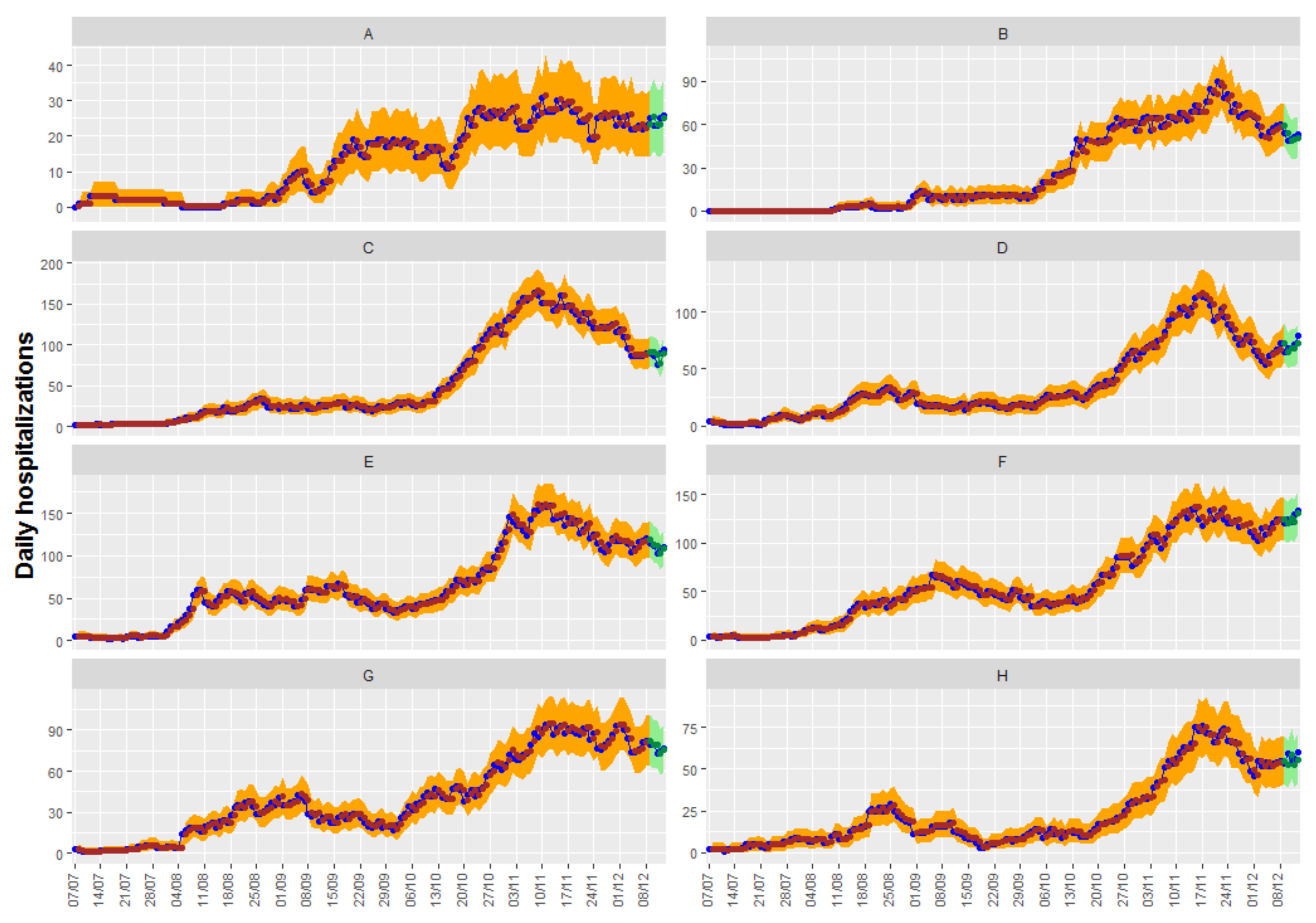
epi.neigbors	3.38%	3.36%

. Once again, results are shown considering the smoothed number of positive new cases at a lag of 9 (Model 2.1) and the smoothed number of new positive cases at lags of 9 and 5 (Model 2.2) as covariates. Individual estimates for the parameters are not shown here because of the quantity of parameters to estimate.

As can be seen in Table 2 and Table 4, there is not much difference between the four models. In all of them, the largest portion of the fitted mean results from the within-area autoregressive component (between 94 and 97%), with very little contribution of cases from adjacent areas and a rather small endemic incidence. There are also no great differences in the goodness of fit parameters provided by the Likelihood inference (Log-likelihood, Akaike Information Criteria (AIC), Bayesian Information Criteria (BIC)), nor in the values of the RMSE.

Figure 6 shows up to 5-day predictions obtained with Model 2.2, together with the fitted and the true observed values. Ninety-five percent confidence intervals can be shown in the graphic for both the predictions and the fitted values.

3.2. Multivariate Covariance Generalized Linear Models

In this section, we apply the MCGLM approach to analyze the multivariate count dataset that was presented in Section 2.1, Equation (5).

As seen in Equation (5), MCGLM takes non-normality into account, defining a variance function and modeling the mean structure by means of a link function and a linear predictor. In this application, we have daily observations from 24 health departments ($K=24$) on N consecutive days, and we model:

$$\begin{array}{c}\hfill g({\mu }_{kt})={\beta }_0+{\beta }_1{x}_{kt}+{\beta }_2{Y}_{k,t-1}+{\beta }_3\sum _{q\ne k}{w}_{qk}{Y}_{q,t-1}+e_{kt},\end{array}$$

(15)

with $g()$ being, in this case, the log-link function and $e_{kt}$ the offset. ${\Sigma }_t$, the covariance matrix is defined as in Equation (7); the Poisson-Tweedie dispersion function is used to model $V({\mu }_t;p_t)$ (Equation (8)), and the matrix linear predictor (Equation (9)) is defined as: $h(\Omega ({\tau }_t))={\tau }_0{I}_{n\times n}+{\tau }_1{Z}_1+{\tau }_2{Z}_2$, where n denotes the total number of observations in the dataset, and $I_{n\times n}$ is the $n\times n$ identity matrix. ${\tau }_0$ is the intercept of the covariance linear model. If $n_t$ denotes the number of observations in time in each spatial region, $Z_1=I_{24\times 24}{⨂}_G{\Gamma }_t$, where ${⨂}_G$ denotes the Kronecker product, and ${\Gamma }_t={(\gamma (i,j))}_{i,j\in \{1,\cdots ,n_t\}}$ with $\gamma (i,j)=1$ if $j\in \{i-1,i+1\}$, and 0 otherwise. ${\tau }_1$ measures the effect of the ’time’. Finally, $Z_2=W{⨂}_G{I}_{n_t\times n_t}$, with W being the spatial adjacency matrix between the 24 health departments.

In this case, we have obtained the best fits when using the exponential covariance link function as $h()$.

We employed a step-wise procedure for selecting the components of the linear predictor. As in the previous modeling, we are going to consider the number of new positive cases at a lag of 9, the number of new positive cases at a lag of 5, and the number of hospitalizations at lag of 1 as potential covariates in Equation (15), and an additional categorical covariate ’Health Department’ to allow different intercepts (${\beta }_{0k}$ instead of ${\beta }_0$) in Equation (15). The population of each health area will also be used as an offset. The SIC using penalty $\delta =2$ and the Wald test were used in the forward and backward steps, respectively. We defined a stopping criterion for the selection procedure as SIC > 0, since the penalty is larger than the score statistics in that case.

In this case, the SIC values indicate that all components, except the value of the daily hospitalizations with a lag of 1 in neighboring regions, should be included in the model (SIC < 0).

To compare the goodness of non-nested models,

Table 5. Goodness of non-nested models, defined from different matrix linear predictors $h(\Omega ({\tau }_t))$.

	$\mathit{h}(\mathsf{\Omega }({\mathit{\tau }}_{\mathit{t}}))=$
	${\mathbf{\tau }}_{\mathbf{0}}{\mathbf{I}}_{\mathbf{K}\times \mathbf{K}}$	${\mathbf{\tau }}_{\mathbf{0}}{\mathbf{I}}_{\mathbf{K}\times \mathbf{K}}+{\mathbf{\tau }}_{\mathbf{1}}{\mathbf{Z}}_{\mathbf{1}}$	${\mathbf{\tau }}_{\mathbf{0}}{\mathbf{I}}_{\mathbf{K}\times \mathbf{K}}+{\mathbf{\tau }}_{\mathbf{1}}{\mathbf{Z}}_{\mathbf{1}}+{\mathbf{\tau }}_{\mathbf{2}}{\mathbf{Z}}_{\mathbf{2}}$
plogLik	−13,540.43	−10,448.25	−10,444.49
df	28	29	30
pAIC	27,136.86	20,954.5	20,948.98
pKLIC	27,138.46	20,958.28	20,954.1
pBIC	27,311.06	21,134.92	21,135.62
RMSEf	13.72	13.62	11.39
RMSEp	16.46	11.77	11.6

provides the pseudo Akaike information criterion (pAIC), the pseudo Bayesian information criterion (pBIC), and the pseudo Kullback-Leibler information criterion (pKLIC) to select the best structure for the matrix linear predictor. According to these results, we will fit the model considering $h(\Omega ({\tau }_t))={\tau }_0{I}_{K\times K}+{\tau }_1{Z}_1+{\tau }_2{Z}_2$.

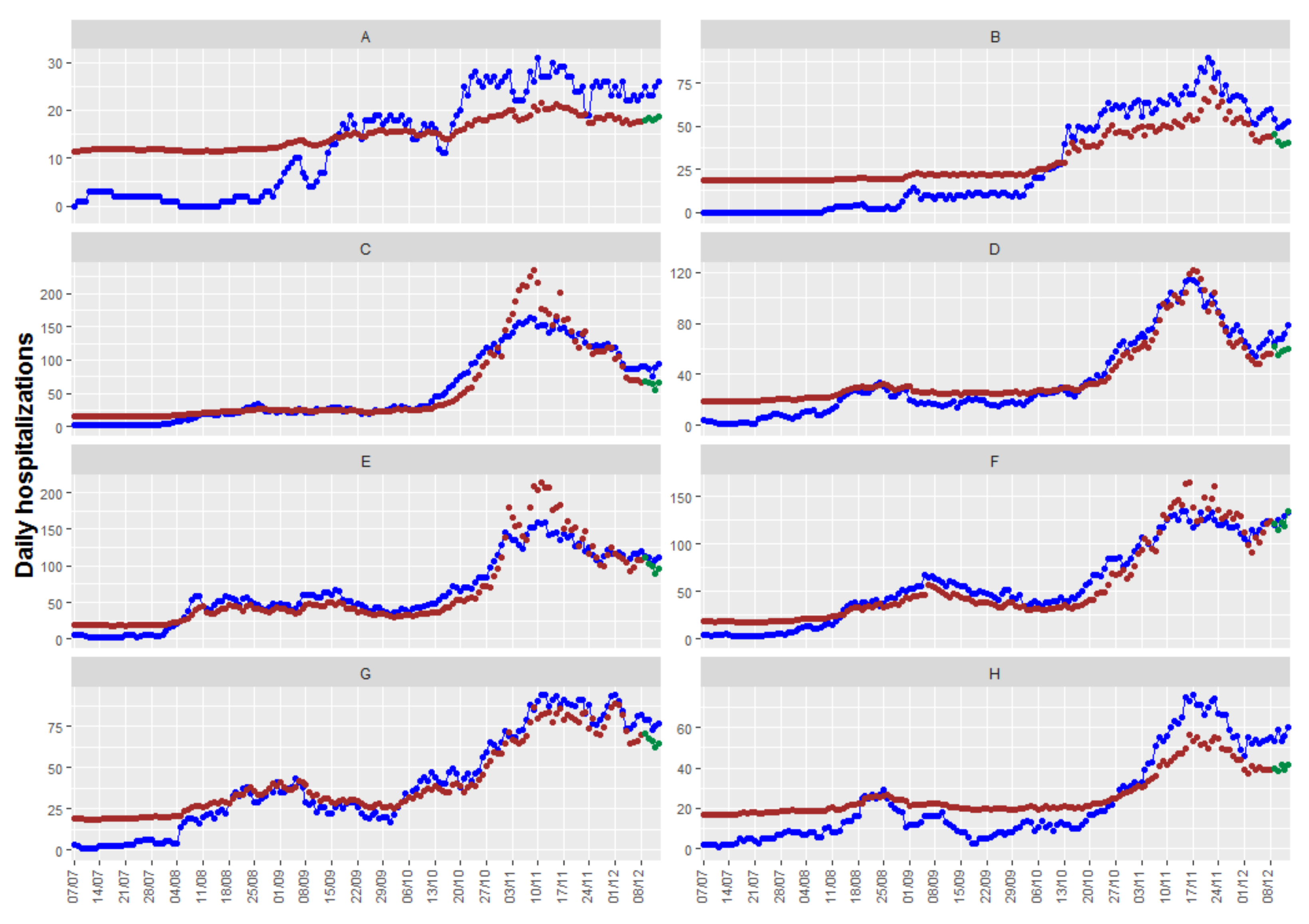
Figure 7 shows the up to 5-day predictions obtained with the resulting model, together with the fitted and the true observed values. In this case, we have obtained an RMSEp equal to 11.6, quite higher than the obtained with the other models/packages. Figure 7 shows that, in this case, there are health departments where the model provides neither a good fit of the observations nor precise predictions, while the fits and predictions of other health departments are very accurate. With the information available, we have not found a model with better fits and predictions for all the health departments.

3.3. Bayesian Spatiotemporal Models

In this section, we apply different models included in the CARBayesST package to the COVID-19 data given in Section 2.1. We start by explaining and justifying the particular cases that can be used.

For the reasons explained in this section, we use the Poisson log-linear model for $Y_{kt}$, Equation (10). Overdispersion cannot be controlled with this package. Although that could be regarded as a handicap, as we will see in the results sections, the adjusted and forecasted values are quite good. In order to induce spatial smoothness between the random effects, we use the binary adjacency matrix W used in previous sections.

Taking into account again the characteristics of our data, the plots shown in Section 2.1, and the fact that our main objective is the prediction of future observations, just two of the spatiotemporal correlation structures included in this package (see Table 1) have been fitted for ${\psi }_{kt}$ in Equation (): the CARar and CAR adaptative structures. Neither spatially varying linear time trend models nor spatiotemporal clustering models are appropriate for our data, and CARanova and CARsepspatial structures assume a symmetric temporal correlation that does not allow us to obtain future predictions.

In both cases, the spatiotemporal structure is modeled with a multivariate first-order autoregressive process with a spatially correlated precision matrix:

$$\begin{array}{ccc}\hfill {\psi }_{kt}& =& {\varphi }_{kt}\hfill \end{array}$$

(16)

$$\begin{array}{ccc}\hfill \hspace{1em}\hspace{1em}\hspace{1em}\hspace{1em}\hspace{1em}\hspace{1em}\hspace{1em} {\varphi }_t|{\varphi }_{t-1}& \sim & N({\rho }_T{\varphi }_{t-1},{\tau }^{2}Q{(W,{\rho }_S)}^{-1})\hfill \\ \hfill {\varphi }_1& \sim & N(0,{\tau }^{2}Q{(W,{\rho }_S)}^{-1}),\hfill \\ \hfill {\tau }^2& \sim & Inverse-Gamma(a,b),\hfill \\ \hfill {\rho }_S,{\rho }_T& \sim & Uniform(0,1),\hfill \end{array}$$

(17)

where ${\varphi }_t=({\varphi }_{1t},\dots ,{\varphi }_{Kt})$ is the vector of random effects for time period t, the precision $Q(W,{\rho }_S)$ corresponds to the CAR models proposed in Reference [67] and has the expression:

$$Q(W,{\rho }_S)={\rho }_S(diag(W\mathbf{1})-W)+(1-{\rho }_S)I,$$

$\mathbf{1}$ is the $K\times 1$ vector of ones, and I the $K\times K$ identity matrix. $({\rho }_S,{\rho }_T)$ respectively control the levels of spatial and temporal autocorrelation, with values of 0 corresponding to independence while a value of 1 corresponds to strong autocorrelation.

The random effects from CARar have a single level of spatial dependence that is controlled by the parameter ${\rho }_S$. That means that all pairs of adjacent areal units will have the same degree of autocorrelation: strongly if ${\rho }_S$ is close to one, while no spatial dependence will exist if ${\rho }_S$ is close to zero.

The CARadaptative model allows for localized spatial autocorrelation, that is, it allows it to be stronger in some parts of the study region. This could be adequate for our data because it would be possible for spatial autocorrelation between adjacent health departments to be correlated or conditionally independent, depending, for example, on whether these departments are in the same big city or according to the socioeconomic characteristics of their inhabitants.

The CARadaptative model allows this spatial autocorrelation heterogeneity by allowing spatially neighboring random effects, which is achieved by modeling the non-zero elements of the neighborhood matrix W as unknown parameters rather than assuming they are fixed constants.

With respect to the covariates to be included in the mean, for the same reasons explained in the previous sections, we again tried two possibilities. Case 1: the smoothed number of new positive cases at a lag of 9. Case 2: the smoothed number of new positive cases at a lag of 9 plus the smoothed number of new positive cases at a lag of 5.

Additionally, as a basic area-specific measure of disease incidence, the population fraction $e_k$ has been also included as an offset.

Inference for all models is based on thinning (by 10) 60,000 posterior samples, including a burn-in period of a further 1000 samples. Convergence plots assured that it was reached in all cases.

Table 6. Deviance information criterion (DIC), effective number of parameters (pd), RMSE of fitted values (RMSEf), and RMSE of predictions (RMSEp) for each model and scenario.

	$\mathit{CARar}$		$\mathit{CARadaptative}$
	Case 1	Case 2	Case 1	Case 2
DIC	18,730.92	18,741.31	18,671.93	18,678.58
pd	793.5918	787.9688	780.8599	770.0481
RMSEf	1.939859	2.027429	1.970366	2.059419
RMSEp	5.610704	5.854628	5.861029	5.402237

displays the overall fit of each model by presenting the deviance information criterion (DIC) and the effective number of parameters (pd). It shows that the adaptive model fits the data better than the pure AR model, with reductions in the DIC in both cases. As a complementary measure of goodness of fit and in order to compare across models, the mean square error of adjusted data (RMSEf) has been also calculated, and it is shown in Table 6. In this case, better results are obtained with the CARar model but as it can be seen the differences are very slight.

The medians of the posterior distribution of each parameter, and its $95\%$ credible intervals are displayed in

Table 7. Medians of the posterior distribution of each parameter and 95% credible intervals for each model and scenario.

	CARar Case 1			CARar Case 2			CARadaptative Case 1			CARadaptative Case 2
	Median	2.5%	97.5%	Median	2.5%	97.5%	Median	2.5%	97.5%	Median	2.5%	97.5%
Intercept	5.7011	5.5108	5.7307	5.6233	5.2602	5.6621	5.6955	5.6223	5.7247	5.6107	5.3673	5.6532
Posit9	0.0022	0.0011	0.0108	0.0027	0.0018	0.0100	0.0022	0.0012	0.0054	0.0028	0.0018	0.0081
Posit5	-	-	-	0.0025	0.0014	0.0097	-	-	-	0.0026	0.0017	0.0075
tau2	0.0225	0.0197	0.0313	0.0222	0.0193	0.0313	0.0136	0.0099	0.0206	0.0128	0.0094	0.0198
rho.S	0.9432	0.8767	0.9591	0.9666	0.9349	0.9784	0.9652	0.9225	0.9774	0.9671	0.9206	0.9792
rho.T	0.9895	0.9811	0.9949	0.9376	0.8420	0.9548	0.9898	0.9836	0.9952	0.9890	0.9824	0.9946
tau2.w	-	-	-	-	-	-	171.0751	98.3797	289.3351	177.6793	104.1783	293.4227

.

As can be seen, the estimated parameters of spatial and temporal correlations show a strong spatial and temporal correlation in all cases. In regard to the covariates, both are significative.

Finally, with respect to the number of step-changes between two spatially adjacent areas detected in the CARadaptative models, only one step change is detected in case 1, while no changes are detected in case 2.

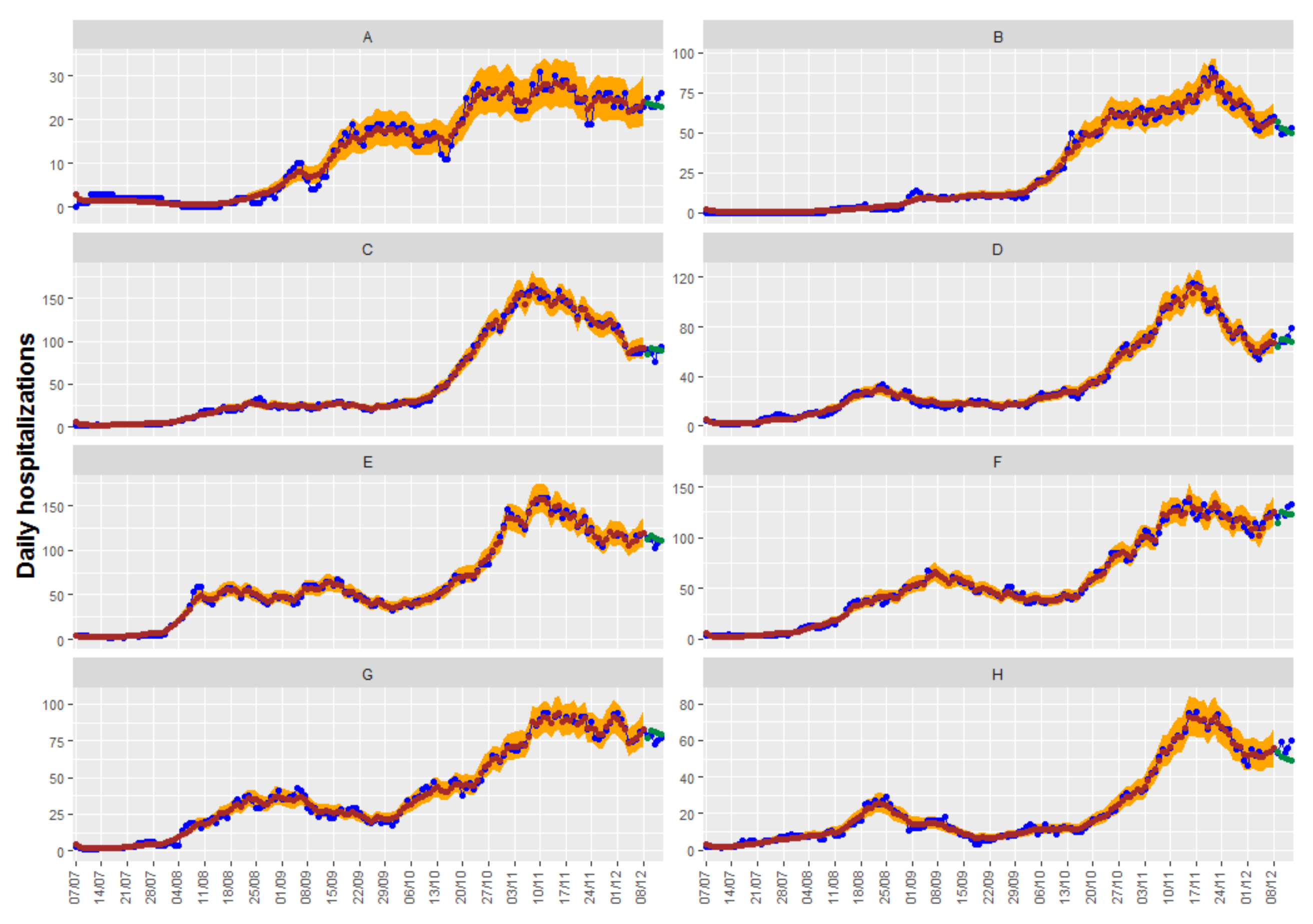
Since our main objective is prediction, we calculate the mean square error of the prediction for up to 5 days for the four cases. These values can be found in the last row of Table 6, and, again, no great differences are observed. In this case, the best result is obtained with the CARadaptative model with both covariates: positive cases at lags of 9 and 5. Adjusted, observed, and predicted values of this model can be seen in Figure 8.

In regard to the credible intervals for the predictions, the CARBasyesST package provides the samples of the posterior distribution of the adjusted data and credible intervals can be easily obtained; they can be seen also in Figure 8.

4. Discussion

Having reviewed and applied the different models, it has been seen that the second model (mcglm package) is the most flexible for modeling the variable of interest, $Y_{kt}$, allowing any type of function of time t in the expression of the mean and a huge variety of spatiotemporal neighborhoods to model both the mean and the variance-covariance matrix (when necessary). The first model (surveillance package) can also use any function of time in the expression of the mean, but the temporal relationship with the neighbors only allows an autoregressive (AR) structure of order 1. This model allows us to choose between a Poisson distribution for modeling the observations or a Negative Binomial model when the data show overdispersion. In regard to modeling, the mean as a function of t, the third model (CARBayesST package) only offers the possibility of linear relationships. In this third model, spatiotemporal relationships between the observations can be introduced into the model of the mean using random effects with different correlation structures.

Having fitted the models, the surveillance package provides the oneStepAhead function to compute successive one-step-ahead predictions for the fitted model, in addition to confident intervals for the predictions and plot methods. However, the other two packages do not have any function implemented to predict future observations from the fitted models, making this process more difficult for non-experts in R programming.

In regard to the estimates of the parameters of the models, significant positive parameters for the covariates are obtained in all cases and the parameters that indicate temporal correlation show high values too for all models. In regard to spatial autocorrelation, there is a difference between the models depending on how the spatial neighborhood has been included in the model. In general, it can be considered that, in order to predict the number of hospitalizations per day, both the number of hospitalizations from the previous day and the number of new cases in the region of interest and in adjacent areas are needed.

Because each type of model has a different methodology that provides different measures of goodness of fit, to compare the performance across different approaches, two common and habitual measures are calculated: the RMSE of the predictions up to 5 days, in order to compare prediction performance between different models, and the RMSE of adjusted data, as a measure of goodness of fit.

With respect to the results, the RMSE of the predictions up to five days of the best model in each package ranges from 5.4 (using the CARBayesST package) to 13.72 (using the mcglm package). There are no large differences between the fitted models using CARBayesST and surveillance packages, ranging, in this case, from 5.4 to 5.78; both values are acceptable in clinical practice. RMSE of fitted data are too excellent using CARBayesST and surveillance (from 0.53 to 1.93), obtaining, in this case, the smallest error with the Endemic-Epidemic model (Equation (14)) (model 2.2).

As was previously explained using Multivariate Covariance generalized Linear Models there are health departments where the model provides neither a good fit of the observations nor precise predictions, while the fits and predictions of other health departments are very accurate. With the information available, we have not found a model with better results for all the health departments. But, as has also been said before, this is the most flexible model for modeling spatiotemporal count data response variables and, probably, good results could have been obtained if there had been more information or in other types of applications.

Concerning the uncertainty of the point estimate predictions, as was explained before, only the surveillance and CARBayesST provided confidence/credible intervals for fitted observations, and just the surveillance package provides them for the forecasts. The intervals are generally slightly wider using the surveillance model than using the Bayesian one. However, using the Bayesian model some observations, are outside of the 95% IC.

These models can truly be used in the current situation. As far as we know, the surveillance package has been used to address several problems related to the COVD-19 pandemic. In fact, the endemic-epidemic models included in the surveillance package, have been applied to a multitude of infectious diseases (see Reference [22] for references), such as Influenza [66], Norovirus [68], and COVID-19 [21,69]. In fact, by July 2021, a regularly updated table of use cases is maintained by S. Meyer at https://github.com/rforge/surveillance/blob/master/www/applications_EE.csv (accessed on 1 June 2021). The CARBayesST package has also been used recently for the study of case-fatality risk due to COVID-19 in Colombia [59].

From the beginning of the 2020, other works have been also focused on modeling the number of COVID-19-related hospitalizations, but as far as we know, all them have objectives, covariates and methodologies different from those seen in our work. Ferstad et al. [70] model the number of people in each county in the United States who are likely to require hospitalization as a result of COVID-19 given the age distribution of the county per the U.S. Census. G. Perone [71] compares several time series forecasting methods to predict the number of patients hospitalized with mild symptoms, and in intensive care units (ICU) in Italy, over the period after 13 October 2020, getting RMSE values greater than ours. Reno et al. [72] model the spread of COVID-19 and its burden on hospital care under different conditions of social distancing in Lombardy and Emilia-Romagna, the two regions of Italy most affected by the epidemic, using a Susceptible-Exposed-Infectious-Recovered (SEIR) deterministic model, which encompasses compartments relevant to public health interventions, such as quarantine. Goic et al. [73] combine autoregressive, machine learning and epidemiological models to provide a short-term forecast of ICU utilization at the regional level in Chile.

Most of them do not provide a goodness of fit measurement that can be used to compare with our results. Only References [70,73] gives values of RMSE. These values are generally greater than the obtained in our work, but they are not directly comparable because their objective is to predict the number of patients hospitalized with mild symptoms, and/or in intensive care units (ICU) separately.

Within the framework of the government support group of the Generalitat Valenciana our models are intended to be used and updated weekly, helping the government make public health decisions, such as the possible need to open new COVID-19 wards in hospitals in the most affected regions.

5. Conclusions

The aim of this work is to review three different spatiotemporal models for count data, implemented in R packages, and to test their performance on an actual case study using three completely different approaches.

Due to these different statistical methodologies, the different packages provide different goodness of fit measures, there being no measure in common between them. Therefore, as the final aim of our case study has been the short-term prediction of the evolution of hospitalizations in the different spatial areas, and the root mean squared prediction error (RMSE) has been obtained in all cases. We can achieve very satisfactory results using each of the packages reviewed, and there is not much difference between them. These results are very promising, particularly in the case of the Valencian Community, but they are also very valuable because they can be applied to any region and the use of these models can be promoted to help in short-term government decision-making regarding preventive measures against the collapse of hospitals. Additionally, they can provide tools to know in advance whether it is necessary to expand hospital capacity in terms of beds and/or workers.

Our objective in this work has not been to say that one package or one type of model is better than others but to show possibilities that can be used in practice to analyze this type of data. The choice of the type of model to use will depend on the application at hand.