Abstract
The objective of this paper is to present a mathematical formalism that states a bridge between physics and psychology, concretely between analytical dynamics and personality theory, in order to open new insights in this theory. In this formalism, energy plays a central role. First, the short-term personality dynamics can be measured by the General Factor of Personality (GFP) response to an arbitrary stimulus. This GFP dynamical response is modeled by a stimulus–response model: an integro-differential equation. The bridge between physics and psychology appears when the stimulus–response model can be formulated as a linear second order differential equation and, subsequently, reformulated as a Newtonian equation. This bridge is strengthened when the Newtonian equation is derived from a minimum action principle, obtaining the current Lagrangian and Hamiltonian functions. However, the Hamiltonian function is non-conserved energy. Then, some changes lead to a conserved Hamiltonian function: Ermakov–Lewis energy. This energy is presented, as well as the GFP dynamical response that can be derived from it. An application case is also presented: an experimental design in which 28 individuals consumed 26.51 g of alcohol. This experiment provides an ordinal scale for the Ermakov–Lewis energy that predicts the effect of a single dose of alcohol.
1. Introduction
Can personality be “dynamic”, i.e., changing through time, and opposed to an unchanging “structure”? The term “structure” as applied to personality has come to connote stability and relative permanence of organization as opposed to states in flux or change, which have been termed “dynamic” [1] (page 293).
On the one hand, research on personality has been based almost entirely on the study of the subject differences in stable traits, which are temporally invariant and can be slightly influenced by situations. This is known as the personality trait perspective. Although this approach has been fruitful and has shown important results about the personality structure, the dynamic aspects of personality have not been sufficiently considered. On the other hand, the social–cognitive approach considers that situations underlie human behavior differences, but it does not accept traits as an explanation of behavior. Both approaches have been competitors, historically [2]. An integrative approach to personality that takes into account both stable and dynamic aspects is necessary. This approach has to incorporate both traits and states, thereby reconciling both the stable and dynamic aspects of personality [3].
There are several integrative models of personality, such as the density distribution approach [4] and the recent Whole Trait Theory [2]. This model asserts that individuals differ not only when regarding their average trait level, but also in how their personality states vary. The network models of personality [5,6,7] are based on the idea that personality emerges from the connective structure of different elements. Moreover, the cognitive-affective processing system (CAPS) model of personality [8,9,10] considers person–situation interactions, and the PersDyn model [3] considers the trajectory of personality states, which is captured by means of three model parameters: baseline, variability, and attractor strength, as well as the temporal order of the states. Finally, the Complex Dynamical Systems model [11] is a dynamical approach that can exhibit complex and unpredictable behavior (chaos).
Observe that these approaches attempt to build bridges between dynamics, fundamental in physics, and personality, fundamental in psychology. In fact, in science, there exists a close attempt to connect dissimilar disciplines, even those whose fields of study seem to be greatly distant, for instance, General Systems Theory (GST) proposed by L. von Bertalanffy [12]. The long-term objective of GST is to construct a universal language common to all scientific disciplines, trying to economize inside knowledge representation and searching for its basic principles. However, a realistic way to reach this objective deals with searching general interdisciplinary theories. A way to obtain these theories is by stating bridges or “isomorphisms” between disciplines. The importance of the bridges or “isomorphisms” in science is emphasized by L. Ferrer [13], who defined them as translations of theories from a discipline to another one because a given problem can be considered as being similar in both of them, or simply by the challenge to open a new theoretical approach.
Therefore, the objective of this paper is to present a bridge between physics and psychology, concretely between analytical dynamics and personality theory, playing a main role in this objective in the concept of energy. This objective tries to answer the question stated at the beginning of the paper: Can personality be “dynamic”, i.e., changing through time, and opposed to an unchanging “structure”? In fact, S. Amigó [14] speculated already about an approach in which energy conservation is a theoretical advancement to explain personality dynamics. However, this paper presents the way to deal with personality energy in a rigorous manner.
Taking into account that here, the concrete person and situation (stimuli that activate behaviors) are considered to be an only system. Thus, to make these sciences converge, a correspondence is proposed: on the one hand, the one between the potential energy and trait as capacity or a disposition to perform some behavior and, on the other hand, the one between the kinetic energy and the dynamic process of the personality system. Thus, we resort to the laws of physics, concretely to analytical dynamics, in order to be applied to psychology. In fact, this approach is not completely new. On one hand, cognition and decision making from the mathematical formalism of quantum mechanics [15] is a good example; on the other hand, certain psychological mechanisms, such as the action and perception, appeal to the principle of free energy imported from thermodynamics [16,17]. Nevertheless, no unified theory of analytical dynamics and thermodynamics has been accepted as definitive, despite the attempts of I. Prigogine, for instance, presented in [18].
The former stage of this paper’s objective was to state a dynamical approach applied to the personality theory based on the work of S. Amigó [14], who stated as an hypothesis the Unique Trait Personality Theory (UTPT). Subsequently, the work [19] presents the psychological validation of the hypothesis stated in [14]. The UTPT claims for a single trait to understand the overall human personality. This single trait is substituted subsequently by the equivalent concept of General Factor of Personality (GFP) in [19] in order to follow the generally accepted scientific term. At present, there is plenty of scientific research in personality that considers that a General Factor of Personality or Big One exists and is situated on top of a hierarchy of personality factors integrating all known personality factors, such as the Big Five [20,21]. In order to measure the GFP, the same authors [19] created a validated questionnaire, the General Factor of Personality Questionnaire (GFPQ). This questionnaire is a good instrument to measure the GFP as a personality stable trait in a trait-format scale. However, the same authors previously developed the Five-Adjective Scale of the General Factor of Personality (GFP-FAS) [22,23], which offers the possibility to measure the GFP dynamical or situational response, composed by five adjectives in a state-format scale [19]. The dimensions of both the GFP and the GFP-FAS are those proposed in [24], that is, a hedonic scale for which units are named activation units (au). The hedonic scale was introduced in reference [24] in order give a dimension (hedonic scale) and a measurement unit (activation unit: au) to the activation level as the physiological base of personality. The interval of variation inside this hedonic scale depends on the particular scale of each adjective of the GFP-FAS. For instance, in the application case presented in Section 5, the hedonic scores vary inside the interval [0, 25] au.
In the last decade, the dynamics of the GFP as a consequence of one or more stimuli have been developed. Concretely, several works studying the GFP short-term and long-term dynamical response to stimulant drugs, such as caffeine, cocaine or methylphenidate, and depressant drugs, such as alcohol, have been studied as well as the equivalent biological bases of personality responses. The works [25,26] provide the references to all these works. Nevertheless, they are also presented in Section 2 in order to highlight the changes in the mathematical structure of the stimulus–response model here presented with respect to a precedent one used in some of those previous works.
In the abovementioned former stage works, the stimulus–response model is presented as a difference–differential equation, i.e., as a discrete-delay differential equation, in which the GFP time derivative is the balance of three terms described in the literature: the homeostatic, excitatory and inhibitory terms (see Section 2 for details). In the referred works, the state-format GFP hedonic scale was applied, and the dynamical response was an inverted U shape followed by a slight U shape, which evolved under a value called “tonic level” to which the dynamics tend asymptotically and play the role of the “attractor strength” described in the PersDyn model [3]. However, in the present work, the stimulus–response model is an integral-differential equation or continuous-delay differential equation. This new approach permits to steer the stimulus–response model to the analytical, dynamics formalism by the suitable mathematical operations.
Summarizing the former stage, it is a dynamical approach to personality theory that deepens into its biological bases [26] and into the dynamical nature of personality, and that focuses on both the general and the individual dynamical responses, in contrast to an exclusive, statistical static approach.
Starting from that first stage, a bridge between physics and psychology can be created, trying to bring to psychology a fundamental principle of physics: the energy conservation principle in the context of psychological reactions to external stimuli (this idea was shortly sketched in [27]). First of all, the stimulus–response model can be converted from an integro-differential equation to a linear second order differential equation. From this new formulation, the analytical dynamics of the stimulus–response model can be developed. On the one hand, the Newtonian formulation, the minimum action principle and the Lagrangian and Hamiltonian functions can be established [28]. Note that it is a straightforward way to state the announced bridge or “isomorphism” between physics and psychology. In fact, the Hamiltonian function provides a first definition of energy as an addition of kinetic energy and potential energy. Concretely, it has the same mathematical structure as the physical problem corresponding to a harmonic oscillator with mass and retrieving parameter, depending on time and being influenced by an external, time-dependent force.
Note that the cause–effect approach given by the integro-differential equation is widened toward the approach given by the minimum action principle for which the dynamics minimize a global function, the action, between two arbitrary times. This new formulation provides an epistemological validation of the stimulus–response model because not all second order differential equations can be derived from a minimum action principle. This is the problem known in the scientific literature as the Inverse Lagrange Problem, i.e., finding a Lagrangian function that produces a known second order differential equation. Classical works, such as [29], show the difficulty of this problem and in many cases, the impossibility to find such a Lagrangian function.
However, the first Hamiltonian function found in this paper is not a conserved amount due to the stimulus time dependence. Nevertheless, the problem can be transformed into a formulation that provides the well-known Ermakov–Lewis invariant [30], which can be reinterpreted as an energy invariant [31]. Thus, starting from our second order differential equation that describes short-term personality dynamics, and following one of the methods presented in [30], an Ermakov–Lewis energy is found, which can be interpreted as a personality energy invariant.
In order to illustrate some of the possibilities for personality theory that this new perspective offers, an application case which refers to an experimental design in which 28 individuals consumed 26.51 g of alcohol (data taken from the work [25]) is presented. Here, the effect of a single dose of alcohol is measured by taking into account both perspectives of personality [1] (page 293): the stable or trait perspective in which the effect of alcohol consumption is measured as the difference between the trait GFP and the baseline of the GFP-FAS; and the flux of change or dynamic perspective in which the effect of alcohol consumption is measured as the difference between the maximum GFP-FAS reached and its baseline. Once an ordinal scale for the Ermakov–Lewis energy has been stated, both measures correlate positively with this scale. Then, the Ermakov–Lewis energy reaches a significant scalar magnitude in order to measure the effects of an alcohol dose. The Ermakov–Lewis energy is also an addition of kinetic and potential energy. Thus, it can be observed that the potential energy has its maximum at the beginning of the experiment, equaling almost completely the total Ermakov–Lewis energy with the kinetic energy being almost zero. Then, it can be observed that both energies exchange their dynamics oscillating around the equilibrium state, whose value coincides statistically with the maximum GFP-FAS reached. In conclusion, this experiment provides evidence that the inference statistics on groups can be applied to Ermakov–Lewis energy, which reaches a predictor scalar magnitude with a stimulus effect.
Regarding the following sections, Section 2 presents the stimulus–response model as an integro-differential equation and the steps to reach a linear second order differential equation as well as its subsequent Newtonian form. Section 3 is devoted to the minimum action principle and the Lagrangian and Hamiltonian formulations, presenting the first non-conserved energy. Section 4 provides the way to get the invariant Ermakov–Lewis energy through suitable changes. Section 5 is devoted to the application case with alcohol and its main results. Section 6 is the conclusion section where some possible future applications are presented.
2. The Stimulus–Response Model and Its Newtonian Form
The stimulus–response model, presented for the first time in [32], is given by the following integro-differential equation:
In Equation (1), the function represents the time dynamics of an arbitrary stimulus and the GFP dynamics, while b and are, respectively, its tonic level and initial value. The dynamics is a balance of three terms, which provide its time derivative as follows:
- The homeostatic control is , i.e., the cause of the fast recovering of the tonic level b to which tends asymptotically; thus, parameter a is named the homeostatic control power. The correct interpretation of tonic level b is important to be stressed: its value is situational and depends on the individual and on the kind of stimulus. However, it plays the same role as the “attractor strength” described in the PersDyn model [3].
- The excitation effect is , which tends to increase the GFP; thus, parameter δ is named the excitation effect power.
- The inhibitor effect is , which tends to decrease the GFP and is the cause of continuously delayed recovering with the weight ; thus, σ is named the inhibitor effect power and τ the inhibitor effect delay. This term makes it such that this stimulus–response model can also be referred to as a continuous-delay differential equation.
Like parameter b, the rest of the model parameters (a, δ, σ and τ) depend on the individual personality or individual biology and on the type of stimulus.
Table 1 presents the dimensions, measurement units and variation intervals of the variables and parameters involved in the stimulus–response model of Equation (1). Note that the time unit depends on the experimental design, due to its units being represented as t (time). In addition, the stimulus dimension and its corresponding units depend on the stimulus’ nature; due to this, they are respectively presented as stimuli (S) and s. In the theoretical application case presented in Section 5, the time units are minutes and, due to the stimulus, has a biochemical nature (alcohol dynamics), its dimensions and units are respectively alcohol amount (AA) and grams (g). The dimension of the GFP is, as presented in Section 1, that proposed in [24], including the hedonic scale (HS), and the corresponding units as activation units (au).

Table 1.
Dimensions, units and the variation intervals of the variables and parameters involved in the stimulus–response model of Equation (1).
Similar stimulus–response models have been presented in the last 13 years. A first theoretical presentation was the one of [24] in which the excitation effect was defined as and the inhibitor effect had a discrete delay as , which converts the model into a difference–differential or discrete-delay differential equation. A generalization toward many doses trying to reproduce the sensitization and habituation effects as well as the cocaine addiction process was provided in [33]. The work [34] is a validation of the abovementioned discrete-delay differential equation with one dose of caffeine, showing how the model can be used as an instrument to predict those individuals inclined to caffeine. The same model was used to predict the GFP response as a consequence of methylphenidate use in the work of [35] and of the self-regulation therapy in [14]. In fact, in the works [35,36], the stimulus–response model also reproduces the c-fos gene dynamical expression as a fundamental biochemical base of personality. The same model was used in [34] to state a dynamical relationship among the Big Five personality factors and the GFP but in the particular case that the inhibitor effect has not a delay, i.e., as instead of . This same simplified approach was used to study the body–mind problem from a dynamical perspective in [37], although the same body–mind problem was deeply studied by including the delay in the model of [26]. Finally, the above cited work [25] dealt with the study of the GFP response to an alcohol dose and how to use the stimulus–response model to predict the effect of a single dose of alcohol.
The stimulus–response model of Equation (1) presents the novelty that the excitation effect is proportional to the stimulus and to the GFP, not only to the stimulus, and that the tonic level is present neither in the excitation effect nor in the inhibitor effect. It was used as a theoretical advancement for the first time in [32] under the hypothesis that being more nonlinear is synonymous to being more adaptable to different responses. This hypothesis was confirmed in the experimental design presented in [38] because Equation (1) can also reproduce dynamical happiness and depression responses. In addition, this new approach permits to steer the stimulus–response model to the analytical dynamics formalism by the suitable mathematical operations that are developed in the next paragraphs and sections.
However, the novelty of the stimulus–response model here presented must be emphasized. It is stated as an integro-differential equation. The previous investigations used difference–differential or discrete-delay differential equations. In addition, the integro-differential equation here presented was just a theoretical proposal in references [27,38], where the applications were quasi-experimental designs. Note, moreover, that in this paper, the integro-differential equation is presented with an application case that is a true experimental design on which statistical inference on a group can be performed (see Section 5).
In the following, in order to get a Newtonian formulation for Equation (1) in this section and a Lagrangian function in Section 3, a second order differential equation equivalent to Equation (1) is needed. To do this, firstly the time derivative is taken in Equation (1):
Subsequently, the term is isolated from Equation (1) and substituted in Equation (2), which, after reorganization, can be written with its initial conditions as follows:
In Equation (3) is the stimulus’ value in the initial time and the following is true:
However, to reach a convenient structure to obtain the Newtonian formulation, Equation (3) must be rewritten in its Sturm–Liouville canonical form by multiplying it by the following factor:
In Equation (6) is an undetermined constant. Thus, Equation (3) becomes the following:
Note that Equation (7) is a version of the stimulus–response model of Equation (1) equivalent to Newton’s second law of dynamics (see [28]). In fact, following Newton’s law, if the momentum is defined as , then Equation (7) can be rewritten as the following:
Equation (8) is the first bridge stated in this paper between physics and psychology. In fact, this is an epistemological approach that must be emphasized: from the initial stimulus–response model that satisfies a cause-and-effect, the Newtonian causal approach of Equation (8) puts the emphasis on the forces that produce changes in the momentum dynamics. More concretely, Equation (8) is equivalent to that of a harmonic oscillator with a time-dependent mass (see Equation (6)), which is non-dimensional, with a time-dependent retrieving parameter with T−2 dimensions and is subjected to the external force with HS·T−2 dimensions (see Table 1). The difference with respect to the physical problem is that, here, the retrieving parameter can take an arbitrary sign during its evolution, while in physics it is always positive.
3. The Minimum Action Principle and the Lagrangian and Hamiltonian Functions
Let us briefly summarize the minimum action principle. In physics, the action S is written as follows [28]:
In Equation (9) are two arbitrary time instants and is the Lagrangian function, which has the dimensions of energy; thus, action S has the dimensions of energy by time. The minimum action principle asserts that, from all the possible trajectories between and , the trajectory that minimizes the action is that which satisfies the Euler–Lagrange equation [26]:
Note that if the Lagrangian L depended on more variables, then every one of these variables would satisfy Equation (10). In our case, the only variable of the formalism is q that represents the GFP dynamics. By the visual inspection of Equation (7), it is easy to deduce that the Lagrangian that holds Equation (10) is as follows:
Observe that the aspect of the Lagrangian corresponds to the most common case in physics: it is a subtraction between a kinetic energy and a potential energy , that is:
The epistemological consequences of this new approach are even more radical than the ones provided by Newton’s equation in Equation (8): the causal principles that take place in every instant in Equation (1) or Equation (8) are reinterpreted from the minimum action principle that minimizes the action globally between two arbitrary time instants, i.e., for all the set of possible trajectories between these two arbitrary time instants. In fact, the minimum action principle is a way to validate epistemologically the presented formalism because not all second order differential equations, such as Equation (8), can be deduced from a minimum action principle. This is the problem known in the scientific literature as the Inverse Lagrange Problem, that is, finding a Lagrangian that produces a known second order differential equation from Euler–Lagrange equations. Classical works, such as [29], show the difficulty of finding a Lagrangian for a determined, second order differential equation. In a similar case to that of Equation (8), the problem reduces itself to find the potential energy .
Advancing in the construction of the bridge between physics and psychology, the momentum p and the Hamiltonian can be defined from the Lagrangian as the following [28]:
Note that Equation (14) is similar to that of a kind of energy in the physical sense because it can be rewritten as follows:
where is the kinetic energy and is the potential energy. In the context of the formalism here presented, the three energies, H, T and V, have the dimensions of HS2·T−2 (see Table 1). However, is not an invariant energy since it is explicitly time-dependent [28]. However, it is possible to get an invariant energy, known in the scientific literature as an Ermakov–Lewis invariant, with suitable changes. This is the goal of the following section.
4. Getting the Invariant Ermakov–Lewis Energy
Ray and Reid’s work [30] provides several methods to get invariants related to Equation (3); these are known as Ermakov–Lewis invariants (note that a collection of invariants can be obtained). Here, we follow what we think is the most intuitive Ray and Reid’s method, which works directly on Equation (3), where the substitution makes it such that the term multiplying vanishes; thus, is non-dimensional, and the variable has the same dimensions as , i.e., HS dimensions (see Table 1). Therefore, the so-called normal form of a second order differential equation is obtained as follows:
where the following is true:
That is, the mentioned change reduces Equations (3)–(16), which is the equation of a harmonic oscillator with frequency and with T−2 dimensions (see Table 1), subjected to a external force with HS·T−2 dimensions (see Table 1). Two new consecutive changes are needed now: the first change on the dependent variable of Equation (16) is , and the second change on the independent variable is , where and are undetermined auxiliary functions by the moment. Observe that if has to conserve the same dimensions as and , then has to have these dimensions, i.e., HS, and has to be non-dimensional (see Table 1). These changes provide the following:
where . In order for Equation (19) to become an equation with constant parameters, we force it to satisfy the following:
where k is an undetermined constant. Note that the variable has the dimensions of time (T), thus it could be interpreted as an intrinsic time of the dynamics that arise as a consequence of the stimulus.
In addition, taking into account Equations (20) and (21), Equation (19) becomes the following:
The Lagrangian, momentum and Hamiltonian corresponding to Equation (22), through the corresponding Euler–Lagrange equations, are as follows:
Note that the Hamiltonian is explicitly time-independent (in which the time is φ); therefore, it is an invariant energy [28], and this is the reason it is also named E. In fact, undoing the above proposed changes, this energy can be expressed in terms of the original variables, arising the known Ermakov–Lewis invariants [30]:
Observe that also Equation (26) is an addition of kinetic energy and potential energy . Thus, as T. Padmanabhan also emphasizes [31], the Ermakov–Lewis invariant E of Equation (26) is invariant energy. In our context, its dimensions are also HS2·T−2 (see Table 1). However, although Te is kinetic energy in Equation (25) with respect to the x variable, it is not “pure kinetic energy” in Equation (26), such as the kinetic energy of Equation (15), because it contains the q variable in addition to its derivative . Nevertheless, it will be referred to as kinetic energy from now onwards. Note, in addition, that and must satisfy Equations (20) and (21), and that Equation (22) can be solved analytically as follows:
Undoing again in Equation (27) the above proposed changes, and assuming that the and auxiliary variables satisfy Equations (20) and (21), the final expression is obtained as follows:
Note that some problems must still be solved: (a) the initial conditions for and to solve, analytically or numerically, Equations (20) and (21); (b) the suitable choice for in Equation (28); and (c) the values of and parameters as well as the value of parameter . In the following, these problems shall try to be solved with a universal aim, i.e., to be independent of the individual and of the type of stimulus.
First of all, in order to choose the initial conditions for and , the following assumptions in in Equation (26) are made: , , , and , which provide , and also provide the initial value of Ermakov–Lewis energy as follows:
Note that Equation (29) is a classical addition of kinetic and potential energy, whose value is conserved for all the GFP evolution period as a consequence of a stimulus.
In addition, the choice of in Equation (28) is clear: the case. The case has the unstable term , and the case has the unstable term . Once the case is chosen as the stable one, the comparison of Equation (28) in with the initial values in Equation (7) provides and with . Observe that finally, one parameter is non-fixed. The preferred option is taking as the free parameter because the parameter (with dimensions T−2) can be considered in future studies as a measure of the resistance of the individual to change his/her personality (as compared with a harmonic oscillator in physics). Then, .
Then, the conclusion is that the Ermakov–Lewis energy of Equation (26) can be written as follows:
Moreover, the dynamics is written as the following:
Note in Equations (30) and (31) that , and that is a free but positive-valued parameter.
5. An Application Case: A Stimulus Given by a Dose of Alcohol
In order to illustrate some of the possibilities for personality theory that this new perspective offers, an application case that refers to an experimental design in which 28 individuals consumed 26.51 g of alcohol (data taken from the work [25]) is used to study personality dynamics as a consequence of a single dose of alcohol consumption. This application case allows observing the following contributions of this theoretical approach inside psychological processes:
- It permits to obtain the personality invariant Ermakov–Lewis energy, generated as a consequence of a stimulus applied to an individual, as an amount of characteristic energy corresponding to the dynamical process.
- It permits to measure the effect of a stimulus through Ermakov–Lewis energy.
- It permits to obtain the dynamics of the kinetic and potential energies that define personality-invariant Ermakov–Lewis energy, as well as its relationship with the tonic level or attractor of the GFP dynamical response to a stimulus.
However, before detailing these contributions, some previous results about the stimulus dynamics are necessary to be presented. In fact, observe that all the theoretical background developed in the previous sections has a general application because it is valid for an arbitrary stimulus . Natural hypotheses for the mathematical structure of the stimulus are that be zero in a determined time or that as . These are, of course, ideal cases because other uncontrolled stimuli can simultaneously have some influence on the individual personality. These ideal cases are similar to those of some problems in physics, for instance, a motion problem when a friction force is not considered because it is negligible. This is the key feature: the negligibility of other stimuli in the sense that they must stay statistically hidden in the GFP evolution caused by the studied stimulus. Conversely, the effects of the studied stimulus on personality would be clearly observable.
In the experiment here considered, the outcomes of the 28 alcohol consumers are calibrated for Equation (1), and the average parameter values are taken as representative of the consumer group. Thus, the effect on the individual personality hides the situational effects of the other stimuli [24,33,36].
To obtain the simplest mathematical structure of alcohol dynamics a two-compartment pharmacokinetics model [39] is considered (alcohol in digestive tube and alcohol in plasma):
In Equation (32), represents the evolution of the ingested alcohol before entering in the organism’s plasma and metabolizing system, being that M is the alcohol initial amount and α the alcohol assimilation rate. In Equation (33), the variable represents the alcohol amount in the organism, assuming that its initial value is , i.e., neither the metabolized nor excreted alcohol of possible previous consumption, and β is the alcohol elimination rate. The coupled differential equations system constituted by Equations (32) and (33) can be integrated, producing the following:
In the considered experiment, the subjects consumed 26.51 g of alcohol, and their GFP was measured every 7 min over 126 min, with the 5-adjective scale of the GFP-FAS in the hedonic scale [22,23,24] inside the interval [0, 25] au, i.e., each adjective was scored inside the interval [0, 5] in the hedonic scale, and the initial condition (baseline) was also measured before consumption. In order to calibrate the model of Equation (1), the assimilation and elimination rate values for alcohol are varied within the following confidence intervals: and (95% confidence), calculated from the outcomes of [40,41]. The results of the model calibration provide the optimal parameter values for each individual and, from them and the corresponding initial values, the Ermakov–Lewis energies can be computed by Equation (29).
From a psychological point of view, the Ermakov–Lewis energy represents the individual dynamics in a direct and more exact way because, being an individual invariant (or an individual conserved energy), it improves the reliability criterion of the dynamical response to a stimulus. Thus, the first step is to present the Ermakov–Lewis energies (E) of the 28 alcohol consumers by their percentiles (PC) as shown in Table 2.
Table 2.
Percentiles (PC) and Ermakov–Lewis energies (E).
In addition, Table 2 permits to consider the Ermakov–Lewis energy as an ordinal variable and then classify its values into three categories by the 33th and 66th percentiles, sorting them from the lesser to the greater category by their scores. Now, the relationship between the Ermakov–Lewis energy and the effect of an alcohol dose can be stated. To do this, let DIFtrait and DIFmax be, respectively, the difference between the trait and the initial value (baseline), and the GFP-FAS maximum reached and the initial value (baseline). Both variables are normally distributed: DIFtrait has a 0.138 Kolmogorov–Smirnov test outcome with a 1.88 signification level, and DIFmax has a 0.11 Kolmogorov–Smirnov test outcome with a 0.2 signification level. In addition, both variables can also be classified into three categories by the 33rd and 66th percentiles, sorting them as well from the lesser to the greater categories by their scores.
On a hand, the relationship between the ordinal Ermakov–Lewis energy and the effect of an alcohol dose from a stable perspective can be set up with the DIFtrait ordinal variable and, on the other hand, the effect of an alcohol dose from a dynamic perspective can be set up with the DIFmax ordinal variable. Table 3 shows both relationships with a gamma test. Both correlations are positive and significant. In addition, these results also show the following: (a) the higher the Ermakov–Lewis energy, the higher the maximum GFP-FAS score; and (b) the lower the initial GFP-FAS score, the higher the Ermakov–Lewis energy involvement in the dynamical process.
Table 3.
Gamma coefficients and statistical significance between the Ermakov–Lewis energy (E) and the DIFtrait and DIFmax variables.
This relationship is strengthened by correlating the categorized Ermakov–Lewis energy as a dependent variable with the non-categorized DIFtrait and DIFmax variables by the Eta and Square Eta tests. See Table 4 in which the differences between the GFP initial condition (or baseline) and the GFP maximum reached (DIFmax) as well as the differences between the GFP initial condition (or baseline) and the GFP trait (DIFtrait), predict a moderated proportion of the Ermakov–Lewis energy variance. Concretely, DIFtrait predicts 47% of the Ermakov–Lewis energy variance, while DIFmax predicts 41% of the Ermakov–Lewis energy variance.
Table 4.
Eta and Square Eta correlations between the categorized Ermakov–Lewis energy (E), as the dependent variable, and the non-categorized DIFtrait and DIFmax variables.
In order to reproduce the representative GFP dynamics of the consumer group, the stimulus–response model of Equation (1) is calibrated for the mean scores of the 28 individuals. Table 5 presents the outcomes of the optimal parameter values, as well as the Ermakov–Lewis energy and its initial kinetic and potential energies. Observe that the initial value of alcohol in plasma is , i.e., the individuals did not consume alcohol prior to testing.
Table 5.
Optimal parameter values, the Ermakov–Lewis energy and its initial kinetic and potential energies for the mean scores of the 28 individuals.
The presented computations and figures were calculated with MATHEMATICA. Figure 1 presents the evolution of the stimulus s(t) given by Equation (34), i.e., the evolution of the alcohol present in the organism during a period four times the period of the experiment (126 min). Observe its trend to zero as .
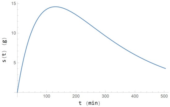
Figure 1.
Evolution of the alcohol present in the organism in a period four times the period of the experiment (126 min).
Figure 2 presents the mean scores of the 28 consumers and the calibrated curve obtained with the stimulus–response model given by the optimal parameter values of Table 5. The evolution period is restricted to that of the experiment (126 min). The GFP initial condition score is 13.29 au and the maximum score reached is 19.07 au. The determination coefficient obtained in the calibration is R2 = 0.986 and an Anderson–Darling test for the residuals show that they distribute normally as N(0, 0.23) with a statistic of 0.14 and a signification level of 0.99, i.e., it is proved that the residuals are white noise.
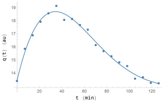
Figure 2.
Evolution of the GFP or for the 28 individuals mean scores (dots) and the calibrated curve (line), in the period of the experiment (126 min).
Figure 3 shows the projection of the same curve for four times the period of the experiment, jointly with its tonic level or attractor b = 19,636 au. Note the trend of the GFP response to this value as . Note also that this representative individual of the group reproduces clearly the response pattern pointed out by the literature as a consequence of alcohol consumption [25], i.e., the inverted U shape GFP response with a recovering period under its initial value and an asymptotic convergence to the tonic level value as , coinciding with the phases of the dynamical response described by the PersDyn model [3].
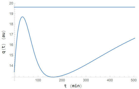
Figure 3.
Evolution of the GFP or q(t) for the calibrated curve and the tonic level b = 19,636 au (upper line), in a period four times that of the experiment, i.e., 4·126 min.
To compute the evolution of the Ermakov–Lewis energy and the kinetic and potential energies given by Equation (30), the and auxiliary variables dynamics are solved numerically by Equations (20) and (21) with the initial values provided in Section 4, taking into account that the free parameter value is chosen as . Then, , i.e., (note that ).
Figure 4 presents the evolution of the Ermakov–Lewis energy with a value (constant), jointly with its kinetic and potential energies.
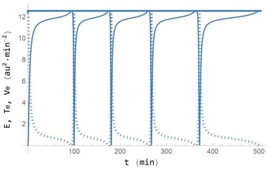
Figure 4.
Ermakov–Lewis energy (E, upper straight line), kinetic energy (Te, first increasing line), and potential energy (Ve, first decreasing dotted line), versus time.
Note in Figure 4 that Te and Ve exchange their dynamics while the Ermakov–Lewis energy (E) keeps constant; in fact this exchange continues for four full blocks. However, what do these blocks mean? To answer this question, note that the time interval of the first block ends at approximately the 98th min, but it corresponds with the score of 13.54 au. Compared with the physical problem of the harmonic oscillator, it is equivalent to the case when the mass runs for half of the period. In addition, in t = 0 min (), the kinetic energy is practically zero, Te = 0.0697 au2·min−2, and the potential energy, Ve = 12.506 au2·min−2, is practically equal to the Ermakov–Lewis energy, E = 12.576 au2·min−2. Thus, after 98 min, these values are recovered with a score of 13.54 au in which Te is, again, practically zero and Ve is practically E. Observe that the GFP score is almost the same and represents the extremes of a harmonic oscillator.
The conclusion is that the GFP maximum score reached, 19.07 au, is identified as the equilibrium point. In other words, the GFP maximum scored reached is the value to which the oscillator tends to return. However, this value is similar to that of the tonic level b = 19,636 au. This is not a coincidence. Let b2 be the categorized variable of the 28 b parameter values. If a gamma test is done between the b2 variable and the reached maximum GFP-FAS variable (categorized), the statistic obtained is γ = 0.722, with a signification level p < 0.001. Thus, statistically, the GFP maximum score reached and the tonic level or attractor are closely related.
Therefore, a general conclusion is that, from the theoretical and practical points of view, Ermakov–Lewis energy represents a central instrument to study personality and its dynamics as a consequence of a stimulus as well as an advanced tool to confirm the predictions of the UTPT [14,24].
6. Conclusions and Future Work
The presented findings about a bridge or “isomorphism” between physics and psychology, concretely between analytical dynamics and personality theory, must be emphasized. The conclusion is that we can apply the energy conservation principle of physics to obtain the state-level personality dynamics produced by some environmental stimuli; in fact, we can consider some psychological mechanisms as analogous to those of physics.
In order to reach these results, on the one hand, the stimulus–response model that has an original integro-differential formulation was reformulated as a Newtonian equation of a harmonic oscillator with one external force acting on it. In addition, the generalized mass and the retrieving force of this harmonic oscillator as well as the referred external force depend on time. Thus, the problem of personality dynamics links with physics in a natural but complex way due to the time-dependencies of the Newtonian formulation on the stimulus–response model.
On the other hand, the link between analytical dynamics and personality theory goes farther because the Newtonian formulation of the stimulus–response model can be deduced from a minimum action principle through the Euler–Lagrange equations. This approach has an important epistemological consequence, that is, in the same way that the natural laws of dynamics are studied by physics, personality dynamics can be studied from a principle that puts its optics in the minimization of a global magnitude, such as action. Moreover, the minimum action principle permits to state Lagrangian and Hamiltonian functions for personality dynamics. The Hamiltonian function is the most important one because it arises as an addition of a kinetic energy and a potential energy as it happens in many cases in physics. Therefore, the link between analytical dynamics and personality theory is further strengthened.
However, the complexity of the Newtonian formulation of the stimulus–response model is translated into the Hamiltonian function, becoming an explicit, time-dependent function and, as a consequence, not being a conserved magnitude. Nevertheless, for approximately the last fifty years, this problem has been studied in physics, and the research studies have provided a way to achieve conserved energy: Ermakov–Lewis energy. Following similar steps of these research studies, Ermakov–Lewis energy can be also obtained for personality dynamics; a new way to obtain results of these dynamics is able to be presented. In fact, an application case for a concrete stimulus, alcohol, is also presented in order to demonstrate that the Ermakov–Lewis energy and the related formalism can be handled mathematically. Therefore, the link between analytical dynamics (physics) and personality theory (psychology) is brought forth.
The application case confirmed the relationship between the kinetic and potential energies of the Ermakov–Lewis energy and the GFP dynamical response, concretely, the relationship between the potential energy and the capacity of an individual to react to a stimulus, as well as the relationship between the stable personality and the kinetic energy. In fact, the invariant Ermakov–Lewis energy was demonstrated to be of central importance to better understand the dynamical response to a stimulus: this characteristic energy amount can be used in inferential statistics, with the sense that a given dynamics can be reduced to a representative scalar, obtaining a relationship between the Ermakov–Lewis energy and the effect of a stimulus, such as an alcohol dose as well as the relationship between the potential and kinetic energies and the tonic level or dynamics’ attractor.
On the other hand, the inspiration obtained from the application cases of the Ermakov–Lewis energy in physics should be also considered. See, for instance, the work [42] for these applications. However, the most important application for the authors is the one related to the quantum approach, for instance, that is considered in the work [43]. In this approach, the tonic level as the asymptotic state in Equation (1) is not considered, and the quantization rules are applied on the Hamiltonian function of Equation (14). Then, a time-dependent Schrödinger equation arises, from which the wave function can be solved analytically in a similar way that is provided for Ermakov–Lewis energy. The wave function provides the quantum version of the Hamilton equations, deduced by D. Bohm and B. J. Hiley [44] from the Schrödinger equation, which are stochastic, and from which quantized trajectories and bifurcations can be studied. Thus, multiple GFP dynamical response patterns and asymptotic states can arise. Therefore, the authors’ hypothesis is that this approach could provide the following: (a) a way to study the normal and the disorder dynamical patterns of personality; and (b) how a bifurcation can steer, as a consequence of a stimulus, from a normal pattern of personality to a disordered one. Then, those sudden changes that many times are observed in personality theory could have a mathematical explanation.
About the limitations of this work, it must be also emphasized that the personality dynamics given by Equation (1) are restricted to the short-term response to a single stimulus. Future research should deal with a stimulus–response model that considers a long-term response, such as the one provided in [33] where addiction and recovering is considered as a consequence of a series of cocaine consumptions with different doses and consumption frequency patterns. Of course, this approach would be more realistic because the processes of sensitization and habituation are observed even in the second dose consumed. However, the study here presented was developed in the same way as the study in [24] that considers a single dose of a stimulant drug. In other words: science normally progresses from easier to more complex approaches.
Other possible future research works can follow different lines. On the one hand, experimental designs to observe the energy of personality in relation to its biological bases should be set up. That is, something similar to, for instance, those works devoted to model the biological responses to a stimulus in relation with personality [26,35,37].
This article cannot be concluded without expressing that, in addition to the methodological and practical applications that the proposal here presented suggests, the finding of conserved energy in psychological processes, specifically in the dynamics of situational personality, assumes something more profound, which is that there exists a temporal symmetry in psychological mechanisms. If the corresponding Ermakov–Lewis Lagrangian is symmetric with respect to time, as it is in our case, according to Noether’s theorem, there must be a conserved quantity, and we have proved it for energy. Symmetry is considered the deepest unifying concept of physics of recent times, being understood as the ultimate foundation of physical laws. Here, it was verified that it can also be the foundation of psychological processes. In fact, Noether’s theorem reproduces the same results for Ermakov–Lewis energy as the dynamical approach here presented, which Ray and Reid [30] also deduced.
In general, the authors consider that the finding here presented is theoretical progress in personality theory from which different applications have to be found in the future. In fact, when a coherent set of ideas, such as those presented in this approach, has been so successful in physics from Newton to the present day, it should be developed until its last theoretical and experimental consequences.
Author Contributions
Conceptualization: A.C., J.C.M. and S.A.; methodology: A.C., J.C.M. and S.A.; software: A.C., J.C.M. and S.A.; validation: A.C., J.C.M. and S.A.; formal analysis: A.C., J.C.M. and S.A.; investigation: A.C., J.C.M. and S.A.; resources: A.C., J.C.M. and S.A.; data curation: A.C., J.C.M. and S.A.; writing—original draft preparation: A.C., J.C.M. and S.A.; writing—review and editing: A.C., J.C.M. and S.A.; visualization: A.C., J.C.M. and S.A.; supervision: A.C., J.C.M. and S.A.; project administration: A.C., J.C.M. and S.A.; funding acquisition: None. All authors have read and agreed to the published version of the manuscript.
Funding
This research received no external funding.
Institutional Review Board Statement
The study was conducted according to the guidelines of the Declaration of Helsinki, and approved by the Ethics Committee of the Universitat Politècnica de València by her president, Amparo Chiralt Boix, in 26 July 2012.
Informed Consent Statement
Informed consent was obtained from all subjects involved in the study.
Data Availability Statement
Data taken from the work [23] are cited below in the References section.
Conflicts of Interest
The authors declare no conflict of interest.
References
- Wiggins, J.S. Personality Structure. Annu. Rev. Psychol. 1968, 19, 293–350. [Google Scholar] [CrossRef] [PubMed]
- Fleeson, W.; Jayawickreme, E. Whole Trait Theory. J. Res. Pers. 2015, 56, 82–92. [Google Scholar] [CrossRef] [PubMed]
- Sosnowska, J.; Kuppens, P.; De Fruyt, F.; Hofmans, J. A dynamic systems approach to personality: The Personality Dynamics (PersDyn) model. Pers. Individ. Differ. 2019, 144, 11–18. [Google Scholar] [CrossRef]
- Fleeson, W. Toward a structure- and process-integrated view of personality: Traits as density distributions of states. J. Pers. Soc. Psychol. 2001, 80, 1011–1027. [Google Scholar] [CrossRef]
- Cervone, D. Personality Architecture: Within-Person Structures and Processes. Annu. Rev. Psychol. 2005, 56, 423–452. [Google Scholar] [CrossRef] [PubMed]
- Cramer, A.O.J.; van der Sluis, S.; Noordhof, A.; Wichers, M.; Geschwind, N.; Aggen, S.H.; Kendler, K.S.; Borsboom, D. Dimensions of Normal Personality as Networks in Search of Equilibrium: You Can’t like Parties if you Don’t like People. Eur. J. Pers. 2012, 26, 414–431. [Google Scholar] [CrossRef]
- Read, S.J.; Monroe, B.M.; Brownstein, A.L.; Yang, Y.; Chopra, G.; Miller, L.C. A neural network model of the structure and dynamics of human personality. Psychol. Rev. 2010, 117, 61–92. [Google Scholar] [CrossRef]
- Mischel, W.; Shoda, Y. A cognitive-affective system theory of personality: Reconceptualizing situations, dispositions, dynamics, and invariance in personality structure. Psychol. Rev. 1995, 102, 246–268. [Google Scholar] [CrossRef] [PubMed]
- Mischel, W.; Shoda, Y. Reconciling processing dynamics and personality dispositions. Annu. Rev. Psychol. 1998, 49, 229–258. [Google Scholar] [CrossRef]
- Mischel, W.; Shoda, Y. Integrating dispositions and processing dynamics within a unified theory of personality: The cognitive–affective personality system. In Handbook of Personality: Theory and Research; Pervin, L.A., John, O.P., Eds.; Guilford Press: New York, NY, USA, 1999; pp. 197–218. [Google Scholar]
- Richardson, M.J.; Dale, R.; Marsh, K.L. Complex dynamical systems in social and personality Psychology: Theory, modeling, and analysis. In Handbook of Research Methods in Social and Personality Psychology, 2nd ed.; Reis, H.T., Judd, C.M., Eds.; Cambridge University Press: Cambridge, UK, 2014; pp. 253–282. [Google Scholar]
- Von Bertalanffy, L.; Sutherland, J.W. General Systems Theory: Foundations, Developments, Applications. IEEE Trans. Syst. Man Cybern. 1974, 4, 592. [Google Scholar] [CrossRef]
- Ferrer, L. Del Paradigma Mecanicista de la Ciencia al Paradigma Sistémico; Universitat de València: Valencia, Spain, 1997. [Google Scholar]
- Amigó, S. La Teoría del Rasgo Único de Personalidad. Hacia una Teoría Unificada del Cerebro y la Conducta (The Unique-Trait Personality Theory. Towards a Unified Theory of Brain and Conduct); Universitat Politècnica de València: Valencia, Spain, 2005. [Google Scholar]
- Pothos, E.M.; Busemeyer, J.R.; Trueblood, J.S. A quantum geometric model of similarity. Psychol. Rev. 2013, 120, 679–696. [Google Scholar] [CrossRef] [PubMed]
- Buckley, C.L.; Kim, C.S.; McGregor, S.; Seth, A.K. The free energy principle for action and perception: A mathematical review. J. Math. Psychol. 2017, 81, 55–79. [Google Scholar] [CrossRef]
- Friston, K.; Kilner, J.; Harrison, L. A free energy principle for the brain. J. Physiol. 2006, 100, 70–87. [Google Scholar] [CrossRef]
- Prigogine, I.; George, C.; Henin, F.; Rosenfeld, L. A Unified Formulation of Dynamics and Thermodynamics (with Special Reference to Non-Equilibrium Statistical Thermodynamics). Chem. Scripta 1973, 4, 5–32. [Google Scholar]
- Amigó, S.; Caselles, A.; Micó, J.C. General Factor of Personality Questionnaire (GFPQ): Only one factor to understand personality? Span. J. Psychol. 2010, 13, 5–17. [Google Scholar] [CrossRef]
- Musek, J. A general factor of personality: Evidence for the Big One in the five-factor model. J. Res. Pers. 2007, 41, 1213–1233. [Google Scholar] [CrossRef]
- Rushton, J.P.; Bons, T.A.; Ando, J.; Hur, Y.-M.; Irwing, P.; Vernon, P.A.; Petrides, K.V.; Barbaranelli, C. A General Factor of Personality From Multitrait–Multimethod Data and Cross–National Twins. Twin Res. Hum. Genet. 2009, 12, 356–365. [Google Scholar] [CrossRef] [PubMed]
- Amigó, S.; Micó, J.C.; Caselles, A. Adjective scale of the unique personality trait: Measure of personality as an overall and complete system. In Proceedings of the 7th Congress of the European Systems Union, Lisboa, Portugal, 17–19 December 2008. [Google Scholar]
- Amigó, S.; Micó, J.C.; Caselles, A. Five adjectives to explain the whole personality: A brief scale of personality. Rev. Int. Sist. 2009, 41–43. Available online: http://www.uv.es/caselles/ (accessed on 2 June 2021).
- Amigó, S.; Caselles, A.; Micó, J.C. A dynamic extraversion model. The brain’s response to a single dose of a stimulant drug. Br. J. Math. Stat. Psychol. 2008, 61, 211–231. [Google Scholar] [CrossRef]
- Amigó, S.; Caselles, A.; Micó, J.C.; Sanz, M.T.; Soler, D. Dynamics of the general factor of personality: A predictor mathematical tool of alcohol misuse. Math. Methods Appl. Sci. 2020, 43, 8116–8135. [Google Scholar] [CrossRef]
- Mico, J.C.; Amigó, S.; Caselles, A.; Romero, P.D. Biology and personality: A mathematical approach to the body-mind problem. Kybernetes 2020. [Google Scholar] [CrossRef]
- Caselles, A.; Amigó, S.; Micó, J.C. Invariant energy in short-term personality dynamics. In Modelling for Engineering & Human Behaviour 2020; Universidad Politécnica de Valencia: Valencia, Spain, 2020; pp. 36–41. [Google Scholar]
- Landau, L.D.; Lifshitz, E.M. Mecánica (Vol. 1 del Curso de Física Teórica); Reverté: Barcelona, Spain, 2002. [Google Scholar]
- Havas, P. The range of application of Lagrangian formalism. Nuovo Cim. 1957, 3, 363–388. [Google Scholar] [CrossRef]
- Ray, J.R.; Reid, J.L. Invariants for forced time-dependent oscillators and generalizations. Phys. Rev. A 1982, 26, 1042–1047. [Google Scholar] [CrossRef]
- Padmanabhan, T. Demystifying the constancy of the Ermakov–Lewis invariant for a time-dependent oscillator. Mod. Phys. Lett. A 2018, 33, 1830005. [Google Scholar] [CrossRef]
- Micó, J.C.; Amigó, S.; Caselles, A. Advances in the general factor of personality dynamics. Rev. Int. Sist. 2018, 22, 34–38. [Google Scholar] [CrossRef]
- Caselles, A.; Micó, J.C.; Amigó, S. Cocaine addiction and personality: A mathematical model. Br. J. Math. Stat. Psychol. 2010, 63, 449–480. [Google Scholar] [CrossRef] [PubMed]
- Caselles, A.; Micó, J.C.; Amigó, S. Dynamics of the General Factor of Personality in Response to a Single Dose of Caffeine. Span. J. Psychol. 2011, 14, 675–692. [Google Scholar] [CrossRef] [PubMed]
- Micó, J.C.; Amigó, S.; Caselles, A. Changing the General Factor of Personality and the c-fos Gene Expression with Methylphenidate and Self-Regulation Therapy. Span. J. Psychol. 2012, 15, 850–867. [Google Scholar] [CrossRef] [PubMed]
- Micó, J.C.; Amigó, S.; Caselles, A. From the Big Five to the General Factor of Personality: A Dynamic Approach. Span. J. Psychol. 2014, 17, 1–18. [Google Scholar] [CrossRef]
- Micó, J.C.; Caselles, A.; Amigó, S.; Cotolí, A.; Sanz, M.T. A Mathematical Approach to the Body-Mind Problem from a System Personality Theory (A Systems Approach to the Body-Mind Problem). Syst. Res. Behav. Sci. 2013, 30, 735–749. [Google Scholar] [CrossRef]
- Amigó, S.; Micó, J.C.; Caselles, A. Methylphenidate and the Self-Regulation Therapy increase happiness and reduce depression: A dynamical mathematical model. In Modelling for Engineering & Human Behaviour 2018; Universidad Politécnica de Valencia: Valencia, Spain, 2018; pp. 6–9. [Google Scholar]
- Byers, J.B.; Sarver, J.G. Pharmacokinetic Modeling. In Pharmacology; Hacker, M., Messer, W., Bachmann, K., Eds.; Academic Press: Cambridge, MA, USA, 2009; pp. 201–277. [Google Scholar]
- Yelland, L.N.; Burns, J.P.; Sims, D.N.; Salter, A.B.; White, J. Inter- and intra-subject variability in ethanol pharmacokinetic parameters: Effects of testing interval and dose. Forensic Sci. Int. 2008, 175, 65–72. [Google Scholar] [CrossRef] [PubMed]
- Holford, N.H.G. Clinical Pharmacokinetics of Ethanol. Clin. Pharmacokinet. 1987, 13, 273–292. [Google Scholar] [CrossRef] [PubMed]
- Espinoza-Padilla, P.B. Ermakov-Lewis Dynamic Invariants with Some Applications. Master’s Thesis, University of Guanajuato, Guanajuato, Mexico, 2000. [Google Scholar]
- Micó, J.C.; Amigó, S.; Caselles, A. A proposal for quantum short time personality dynamics. In Modelling for Engineering & Human Behaviour 2020; Universidad Politécnica de Valencia: Valencia, Spain, 2020; pp. 102–108. [Google Scholar]
- Bohm, D.; Hiley, B.J.; Goldstein, S. The Undivided Universe: An Ontological Interpretation of Quantum Theory; Routledge: London, UK; New York, NY, USA, 1995. [Google Scholar]
Publisher’s Note: MDPI stays neutral with regard to jurisdictional claims in published maps and institutional affiliations. |
© 2021 by the authors. Licensee MDPI, Basel, Switzerland. This article is an open access article distributed under the terms and conditions of the Creative Commons Attribution (CC BY) license (https://creativecommons.org/licenses/by/4.0/).