Lie Symmetry Analysis, Self-Adjointness and Conservation Law for a Type of Nonlinear Equation

Abstract

In the present paper, we mainly focus on the symmetry of the solutions of a given PDE via Lie group method. Meanwhile we transfer the given PDE to ODEs by making use of similarity reductions. Furthermore, it is shown that the given PDE is self-adjoining, and we also study the conservation law via multiplier approach.

1. Introduction

When investigating the classification of the solutions of differential equations, Sophus Lie introduced the notion of the continuous transformation group, which was named the Lie group by the following people in memory of him. Afterwards, the application of Lie groups has been developed by lots of mathematicians, such as Ovsiannikov [1], Ibragimov [2], Olver [3] and Bluman et al. [4,5]. Symmetry is one of the intrinsic features of a partial differential equation (PDE). Lie group analysis is one of the most powerful methods to study the symmetry of their solutions. Based on the symmetries of a PDE, many other properties of the equation, such as exact solutions to conservation laws can be successively considered. In any case, another method to solve the nonlinear evolution equation (such as Burgers equation) is to use Hopf cole transformation in a high order spectral column setting [6,7].

The conservation laws (Cls) have drawn great attention from the mathematical physicists. In the past few decades, many methods for dealing with the Cls were derived, the most famous being Noether’s approach [8], multiplier approach and Ibragimov’s method [9]. Moreover, Cls for nonlinearly self-adjoint systems can be constructed systematically by pairs of symmetries and adjoint symmetries. In particular, ref. [10] supplies the most general connection between Cls and pairs of symmetries and adjoint symmetries for non-self-adjoint systems. On the contribution of the Lie symmetry method, significant studies have been performed on the integrability of the nonlinear PDEs, group classification, optimal system, reduced solutions and conservation laws, such as [11,12,13,14,15,16,17,18,19,20,21,22,23], and references therein.

In [24,25], a new completely integrable equation

$$m_t=\frac{1}{2}{\left(\frac{1}{m^2}\right)}_{xxx}-\frac{1}{2}{\left(\frac{1}{m^2}\right)}_x.$$

(1)

was proposed. It was shown that this equation has no smooth solitons and it has bi-Hamiltonian structure and Lax pair. At the end of [25], Qiao introduced a more general PDE

$$m_t=\frac{1}{2}{\left(\frac{1}{m^k}\right)}_{xxx}-\frac{1}{2}{\left(\frac{1}{m^k}\right)}_x.$$

(2)

with a constant $k\in \mathbb{R}$.

If $k=0$, it is a trivial case; if $k=-1$, it is a linear case; if $k=\frac{1}{2}$, it is a Harry–Dym case; if $k=2$, it is reduced to (1). Unless explicitly stated, throughout this paper we always assume $k\ne 0,-1$. Sakovich in [26] supplied a transformation which was used to derive smooth soliton solutions of the new equation from the known rational and soliton solutions of the old one. To the authors’ knowledge, the Lie symmetry analysis, self-adjointness and conservation laws of (2) have not been studied. In this paper, we mainly focus on the above aspects on (2) for $k\ne 0,-1$.

If we perform the transformation $u(x,t)=\frac{1}{m(x,t)}$, Equation (2) is reduced to

$$u_t+\frac{k(k-1)(k-2)}{2}{u}^{k-1}{u}_x^3+\frac{3k(k-1)}{2}{u}^k{u}_x{u}_{xx}+\frac{k}{2}{u}^{k+1}{u}_{xxx}-\frac{k}{2}{u}^{k+1}{u}_x=0.$$

(3)

From now on, we will focus on the study of Equation (2), which is equivalent to that of Equation (2).

2. Lie Symmetries of Equation (2)

In this section, we shall investigate the Lie symmetry analysis of Equation (2).

First of all, let us consider the Lie group of point transformations

$$\begin{array}{cc}\hfill & x^{*}=x+\epsilon \xi (x,t,u)+O({\epsilon }^2),\hfill \\ \hfill & t^{*}=t+\epsilon \tau (x,t,u)+O({\epsilon }^2),\hfill \\ \hfill & u^{*}=u+\epsilon \varphi (x,t,u)+O({\epsilon }^2),\hfill \end{array}$$

(4)

with a small parameter $\epsilon \ll 1$. The vector field associated with the above transformation group of transformations can expressed as

$$V=\xi (x,t,u)\frac{\partial }{\partial x}+\tau (x,t,u)\frac{\partial }{\partial t}+\varphi (x,t,u)\frac{\partial }{\partial u},$$

(5)

where $\xi (x,t,u)$, $\tau (x,t,u)$ and $\varphi (x,t,u)$ are coefficient functions of the vector field to be determined.

Theorem 1.

For the arbitrary real parameter k, if $k\ne 0,-1$, the complete group classification of Equation (2) is as follows: $(1)$ If $k\ne \frac{1}{2}$, the vector field of Equation (2) is

$$V_1=\frac{\partial }{\partial x},V_2=\frac{\partial }{\partial t},V_3=-(k+1)t\frac{\partial }{\partial t}+u\frac{\partial }{\partial u}.$$

(6)

$(2)$ If $k=\frac{1}{2}$, the vector field of Equation (2) is

$$\begin{array}{c}{V}_1=\frac{\partial }{\partial x},V_2=\frac{\partial }{\partial t},V_3=-\frac{3}{2}t\frac{\partial }{\partial t}+u\frac{\partial }{\partial u},\hfill \\ V_4=\frac{1}{2}{e}^x\frac{\partial }{\partial x}+e^{x}u\frac{\partial }{\partial u},V_5=-\frac{1}{2}{e}^{-x}\frac{\partial }{\partial x}+e^{-x}u\frac{\partial }{\partial u}.\hfill \end{array}$$

(7)

Proof. 

The third prolongation of V is

$$\begin{array}{cc}\hfill & {\mathrm{pr}}^{(3)}V=V+{\varphi }^x\frac{\partial }{\partial u_x}+{\varphi }^t\frac{\partial }{\partial u_t}+{\varphi }^{xx}\frac{\partial }{\partial u_{xx}}+{\varphi }^{xt}\frac{\partial }{\partial u_{xt}}+{\varphi }^{tt}\frac{\partial }{\partial u_{tt}}\\ \hfill & +{\varphi }^{xxx}\frac{\partial }{\partial u_{xxx}}+{\varphi }^{xtt}\frac{\partial }{\partial u_{xtt}}+{\varphi }^{xxt}\frac{\partial }{\partial u_{xxt}}+{\varphi }^{ttt}\frac{\partial }{\partial u_{ttt}},\end{array}$$

(8)

where the explicit expressions of unknown functions ${\varphi }^t,{\varphi }^x,{\varphi }^{xx},{\varphi }^{xxx}$ are as follows

$$\begin{array}{cc}\hfill {\varphi }^t& =D_t(\varphi -\xi u_x-\tau u_t)+\xi u_{xt}+\tau u_{tt},\hfill \end{array}$$

(9)

$$\begin{array}{cc}\hfill {\varphi }^x& =D_x(\varphi -\xi u_x-\tau u_t)+\xi u_{xx}+\tau u_{xt},\hfill \end{array}$$

(10)

$$\begin{array}{cc}\hfill {\varphi }^{xx}& =D_x^2(\varphi -\xi u_x-\tau u_t)+\xi u_{xxx}+\tau u_{xxt},\hfill \end{array}$$

(11)

$$\begin{array}{cc}\hfill {\varphi }^{xxx}& =D_x^3(\varphi -\xi u_x-\tau u_t)+\xi u_{xxxx}+\tau u_{xxxt}.\hfill \end{array}$$

(12)

In (9)–(12), $D_x$ and $D_t$ are both total derivatives with respect to $x,t$, respectively. We denote the left hand side of Equation (2) by $\Delta$. In view of ${\mathrm{pr}}^{(3)}{V(\Delta )|}_{\Delta =0}=0$, we obtain

$$\begin{array}{ccc}0\hfill & =\hfill & {\varphi }^t+\frac{k{(k-1)}^2(k-2)}{2}{u}^{k-2}\varphi u_x^3+\frac{3k(k-1)(k-2)}{2}{u}^{k-1}{\varphi }^x{u}_x^2\hfill \\ \hfill & \hfill & +\frac{3k^2(k-1)}{2}{u}^{k-1}\varphi u_x{u}_{xxx}+\frac{3k(k-1)}{2}{u}^k{\varphi }^x{u}_{xx}+\frac{3k(k-1)}{2}{u}^k{\varphi }^{xx}{u}_x\hfill \\ \hfill & \hfill & +\frac{k(k+1)}{2}{u}^k\varphi u_{xxx}+\frac{k}{2}{u}^{k+1}{\varphi }^{xxx}-\frac{k(k+1)}{2}{u}^k\varphi u_x-\frac{k}{2}{u}^{k+1}{\varphi }^x.\hfill \end{array}$$

(13)

We substitute (9)–(12) into (8) and replace $u_t$ by

$$-\left(\frac{k(k-1)(k-2)}{2}{u}^{k-1}{u}_x^3+\frac{3k(k-1)}{2}{u}^k{u}_x{u}_{xx}+\frac{k}{2}{u}^{k+1}{u}_{xxx}-\frac{k}{2}{u}^{k+1}{u}_x\right)$$

whenever it appears in (13) and divide it into several cases to discuss it.

Firstly we assume $k\ne 1,2$. By solving (13), one can get following forms for the infinitesimal elements $\xi ,\tau ,\varphi$:

$$\left\{\begin{array}{c}{\tau }_x={\tau }_u=0,\tau =\tau (t),\hfill \\ {\xi }_u=0,{\varphi }_{uu}=0,\hfill \\ u{\tau }_t+(k+1)\varphi -3u{\xi }_x=0,\hfill \\ u{\varphi }_u+u{\tau }_t+k\varphi -3u{\xi }_x=0,\hfill \\ 2u{\varphi }_u+u{\tau }_t+(k-1)\varphi -3u{\xi }_x=0.\hfill \end{array}\right.$$

(14)

If $k\ne \frac{1}{2}$, Equation (14) implies $\xi =c,\tau =-(k+1)at+b,\varphi =au$, which yields the vector fields in (6).

If $k=\frac{1}{2}$, Equation (14) implies

$$\begin{array}{c}\xi =\frac{1}{2}{c}_1{e}^x-\frac{1}{2}{c}_2{e}^{-x}+c_4,\hfill \\ \tau =-\frac{3}{2}{c}_{3}t+c_5,\hfill \\ \varphi =(c_1{e}^x+c_2{e}^{-x}+c_3)u,\hfill \end{array}$$

which yields the vector fields in (7).

Secondly, we assume $k=1$ or $k=2$, similar process yields the vector fields in (6). □

It is necessary to check that the vector fields form a Lie algebra, respectively. Taking (7) as an example,

$$\begin{array}{cc}\hfill & [V_1,V_2]=0,[V_1,V_3]=0,[V_1,V_4]=V_4,[V_1,V_5]=-V_5,\hfill \\ \hfill & [V_2,V_3]=-\frac{3}{2}{V}_2,[V_2,V_4]=0,[V_2,V_5]=0,[V_3,V_4]=0,\hfill \\ \hfill & [V_3,V_5]=0,[V_4,V_5]=\frac{1}{2}{V}_1.\hfill \end{array}$$

We denote this Lie algebra by $\mathfrak{L}$. If we drop the relation in (7) of $V_1,\cdots ,V_5$, it will be an abstract Lie algebra. The vector fields corresponding to $V_1,\cdots ,V_5$ supply a Lie algebra representation of $\mathfrak{L}$ (see [27]). In addition, $\mathfrak{L}$ can be decomposed as $\mathfrak{L}=\mathfrak{s}\oplus \mathfrak{n}$, where $\mathfrak{s}=\mathrm{span}\{V_1,V_4,V_5\}$ denotes the simple ideal of $\mathfrak{L}$, $\mathfrak{n}=\mathrm{span}\{V_2,V_3\}$ stands for the nilpotent subalgebra of $\mathfrak{L}$.

As we know, infinitesimal generators $V_i$ generate the one-parameter transform groups, by solving the following ordinary differential equations with the initial conditions:

$$\begin{array}{c}\frac{d{x}^{*}}{d\epsilon }=\xi (x^{*},t^{*},u^{*}),x^{*}{|}_{\epsilon =0}=x,\hfill \\ \frac{d{t}^{*}}{d\epsilon }=\tau (x^{*},t^{*},u^{*}),t^{*}{|}_{\epsilon =0}=t,\hfill \\ \frac{d{u}^{*}}{d\epsilon }=\varphi (x^{*},t^{*},u^{*}),u^{*}{|}_{\epsilon =0}=u,\hfill \end{array}$$

it follows the case $k\ne \frac{1}{2}$

$$\begin{array}{cc}\hfill & G_1:(x,t,u)⟼(x+\epsilon ,t,u),\hfill \end{array}$$

(15)

$$\begin{array}{cc}\hfill & G_2:(x,t,u)⟼(x,t+\epsilon ,u),\hfill \end{array}$$

(16)

$$\begin{array}{cc}\hfill & G_3:(x,t,u)⟼(e^{\epsilon }x,e^{-(k+1)\epsilon }t,e^{\epsilon }u),\hfill \end{array}$$

(17)

and case $k=\frac{1}{2}$

$$\begin{array}{cc}\hfill & G_1:(x,t,u)⟼(x+\epsilon ,t,u),\hfill \end{array}$$

(18)

$$\begin{array}{cc}\hfill & G_2:(x,t,u)⟼(x,t+\epsilon ,u),\hfill \end{array}$$

(19)

$$\begin{array}{cc}\hfill & G_3:(x,t,u)⟼\left(e^{\epsilon }x,e^{-\frac{3}{2}\epsilon }t,e^{\epsilon }u\right),\hfill \end{array}$$

(20)

$$\begin{array}{cc}\hfill & G_4:(x,t,u)⟼\left(x-ln(2-\epsilon e^x)+ln2,t,\frac{4u}{{(2-\epsilon e^x)}^2}\right),\hfill \end{array}$$

(21)

$$\begin{array}{cc}\hfill & G_5:(x,t,u)⟼\left(x+ln(2-\epsilon e^{-x})-ln2,t,\frac{4u}{{(2-\epsilon e^{-x})}^2}\right).\hfill \end{array}$$

(22)

Remark 1.

Any solution of Equation (2) when $k\ne \frac{1}{2}$ is invariant under the operation of G${}_1$, G${}_2$, G${}_3$ and their products in (15)–(17).

Any solution of Equation (2) when $k=\frac{1}{2}$ is invariant under the operation of G${}_1$–G${}_5$ and their products in (18)–(22).

Remark 2.

If $k\ne \frac{1}{2}$, Equation (2) is also invariant under the operation of the prolongations of $V_1$–$V_3$. We take $V_3$ as an example, since the prolongations of $V_1$ and $V_2$ are trivial.

$${\mathrm{pr}}^{(3)}{V}_3(\Delta )=(k+2)\Delta .$$

Remark 3.

If $k=\frac{1}{2}$, Equation (2) is invariant under the operation of the prolongations of $V_1$–$V_5$. For instance

$${\mathrm{pr}}^{(3)}{V}_4(\Delta )=e^x\Delta ,{\mathrm{pr}}^{(3)}{V}_5(\Delta )=e^{-x}\Delta .$$

3. Similarity Reductions for Equation (2)

In this section, we shall construct the similarity variables so as to deal with the symmetry reduction, which transfer the PDE into ODE. Considering the fact that the vector fields of $k\ne \frac{1}{2}$ and $k=\frac{1}{2}$ are partly the same, we shall discuss them together.

$(1)$ For the generator $V_1$, we assume $\zeta =t$, $u=f(\zeta )$ and obtain the trivial solution $f=c$, where c is an arbitrary nonzero constant.

$(2)$ For the linear combination $V_2$, we have

$$u=f(\zeta ),$$

(23)

where $\zeta =x$. Substituting (23) into Equation (2), we can get

$$(k-1)(k-2)f^{\prime 3}-3(k-1)f{f}^{\prime }{f}^{″}+f^2{f}^{‴}-f^2{f}^{\prime }=0,$$

(24)

where $f^{{}^{\prime }}=\frac{df}{d\zeta }$.

$(3)$ For the generator $V_3$, we have

$$u=t^{-\frac{1}{k+1}}f(\zeta ),$$

(25)

where $\zeta =x$. Substituting (25) into Equation (2), we arrive at

$$-\frac{1}{k+1}f+\frac{k(k-1)(k-2)}{2}{f}^{k-1}{f}^{\prime 3}-\frac{3k(k-1)}{2}{f}^k{f}^{\prime }{f}^{″}+\frac{k}{2}{f}^{k+1}{f}^{{}^{‴}}-\frac{k}{2}{f}^{k+1}{f}^{{}^{\prime }}=0,$$

(26)

where $f^{{}^{\prime }}=\frac{df}{d\zeta }$.

$(4)$ For the generator $V_4$, we have

$$u=f(\zeta )e^{2x},$$

(27)

where $\zeta =t$. By substituting (27) into Equation (2), we get the trivial solution $f=c$, where c is an arbitrary nonzero constant.

$(5)$ For the generator $V_5$, we have

$$u=f(\zeta )e^{-2x},$$

(28)

where $\zeta =t$, we get the trivial solution $f=c$, where c is an arbitrary nonzero constant.

The ODEs (24) and (26) hold for arbitrary k, including ${\displaystyle \frac{1}{2}}$, but the similarity reductions of $V_4$ and $V_5$ only belong to the equation when ${\displaystyle k=\frac{1}{2}}$.

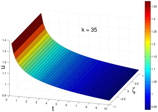
In the above, we sketch the graphs of $f(\xi )$ in Equations (24) and (26) and 3D-plot of $u(x,t)$ in Equations (23)–(26) under initial conditions $f(0)=\frac{3}{2},f(1)=1,f^{\prime }(0)=0$. Please refer to Figure 1, Figure 2, Figure 3, Figure 4, Figure 5 and Figure 6.

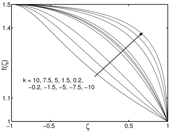
Figure 1. The graph of $f(\xi )$ given by Equation (24) as k near 0.

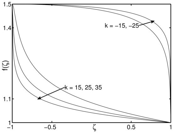
Figure 2. The graph of $f(\xi )$ given by Equation (24) as k approaching $-\infty$ and $+\infty$.

Figure 3. The graph of $u(x,t)$ given by Equations (23) and (24) for $k=0.5$.

Figure 4. The graph of $u(x,t)$ given by Equations (23) and (24) for $k=2$.

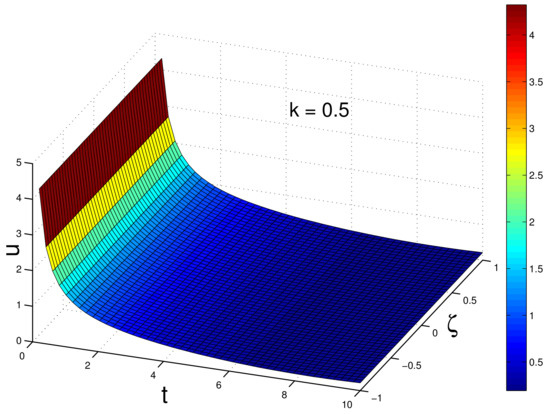
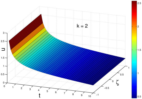
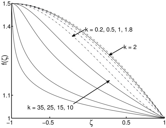
Figure 5. The graph of $f(\xi )$ given by Equation (26) as k near 0.

Figure 6. The graph of $u(x,t)$ given by Equations (25) and (26) for $k=35$.

4. Nonlinear Self-Adjointness and Conservation Law

For given PDEs

$$R^{\beta }(x,u,u_{(1)},\cdots ,u_{(k)})=0,$$

(29)

define the Euler–Lagrange operator

$$\frac{\delta }{\delta u^{\alpha }}\equiv \frac{\partial }{\partial u^{\alpha }}+\sum _{j=1}^{\infty }{(-1)}^j{D}_{i_1}\cdots D_{i_j}\frac{\partial }{\partial u_{i_1\cdots i_j}^{\alpha }},\alpha =1,2,\cdots ,m,$$

(30)

and the formal Lagrangian

$$\mathcal{L}=\sum _{\beta =1}^m{v}^{\beta }{R}^{\beta }(x,u,u_{(1)},\cdots ,u_{(k)}).$$

(31)

The adjoint equations is given by

$${(R^{\alpha })}^{\ast }(x,u,u_{(1)},\cdots ,u_{(k)})=\frac{\delta \mathcal{L}}{\delta u^{\alpha }}=0,\alpha =1,2,\cdots ,m,v=v(x).$$

(32)

Theorem 2.

The differential Equation (2) is self-adjoining if and only if $k\ne 1$.

Proof. 

It is obvious that $\alpha =1$ and $R^{\alpha }(x,u,u_{(1)},\cdots ,u_{(k)})=\Delta (x,t,u,u_t,u_x,u_{xx},u_{xxx})$. The formal Lagrangian is

$$\mathcal{L}=v\left(u_t+\frac{k(k-1)(k-2)}{2}{u}^{k-1}{u}_x^3+\frac{3k(k-1)}{2}{u}^k{u}_x{u}_{xx}+\frac{k}{2}{u}^{k+1}{u}_{xxx}-\frac{k}{2}{u}^{k+1}{u}_x\right).$$

(33)

Substituting it into $\frac{\delta }{\delta u}=0$, we have the adjoint equation of Equation (2)

$$\begin{array}{c}k(k-1)(k-2)u^{k-2}v{u}_x^3-\frac{k}{2}{u}^{k+1}{v}_{xxx}-3k{u}^{k-1}{v}_x{u}_x^2+3k(k-2)u^{k-1}v{u}_x{u}_{xx}\hfill \\ +\frac{k}{2}{u}^{k+1}{v}_x-3k{u}^k{v}_{xx}{u}_x-3k{u}^k{v}_x{u}_{xx}-v_t=0.\hfill \end{array}$$

(34)

By means of

$$\begin{array}{c}[k(k-1)(k-2)u^{k-2}v{u}_x^3-\frac{k}{2}{u}^{k+1}{v}_{xxx}-3k{u}^{k-1}{v}_x{u}_x^2+3k(k-2)u^{k-1}v{u}_x{u}_{xx}\hfill \\ +\frac{k}{2}{u}^{k+1}{v}_x-3k{u}^k{v}_{xx}{u}_x-3k{u}^k{v}_x{u}_{xx}-v_t{]|}_{v=\phi (x,t,u)}=\lambda \Delta ,\hfill \end{array}$$

we have

$$\phi =\left\{\begin{array}{c}(c_1{e}^x+c_2{e}^{-x}+c_3)u^{-2},\mathrm{if}k\ne 1,\hfill \\ 0,\mathrm{if}k=1,\hfill \end{array}\right.$$

(35)

which completes the proof. □

We will now investigate the conservation law for Equation (2) by multiplier. For the differential Equation (29) with $\beta =1$, we suppose $\mathsf{\Lambda }=\mathsf{\Lambda }(x,u)$ is its multiplier and $T^i$’s are its conserve vectors, then $\mathsf{\Lambda }$ satisfies the property

$$D_i{T}^i=\mathsf{\Lambda }E.$$

(36)

By (35) and (36), we have

$$\begin{array}{c}\left[(c_1{e}^x+c_2{e}^{-x}+c_3)u^{-2}\right][u_t+\frac{k(k-1)(k-2)}{2}{u}^{k-1}{u}_x^3+\frac{3k(k-1)}{2}{u}^k{u}_x{u}_{xx}\hfill \\ +\frac{k}{2}{u}^{k+1}{u}_{xxx}-\frac{k}{2}{u}^{k+1}{u}_x]\hfill \\ =D_x[c_1\left(\frac{k(k-1)}{2}{u}^{k-2}{e}^x{u}_x^2+\frac{k}{2}{u}^{k-1}{e}^x{u}_{xx}-\frac{k}{2}{u}^{k-1}{e}^x{u}_x\right)\hfill \\ +c_2\left(\frac{k(k-1)}{2}{u}^{k-2}{e}^{-x}{u}_x^2+\frac{k}{2}{u}^{k-1}{e}^{-x}{u}_{xx}+\frac{k}{2}{u}^{k-1}{e}^{-x}{u}_x\right)\hfill \\ +c_3\left(\frac{k(k-1)}{2}{u}^{k-2}{u}_x^2+\frac{k}{2}{u}^{k-1}{u}_{xx}-\frac{1}{2}{u}^k\right)]\hfill \\ +D_t\left[-\left(c_1{e}^x+c_2{e}^{-x}+c_3\right)u^{-1}\right].\hfill \end{array}$$

Therefore the conserved vectors for Equation (2) are

$$\begin{array}{c}{T}_1^x=\frac{k(k-1)}{2}{u}^{k-2}{e}^x{u}_x^2+\frac{k}{2}{u}^{k-1}{e}^x{u}_{xx}-\frac{k}{2}{u}^{k-1}{e}^x{u}_x,T_1^t=-e^x{u}^{-1},\hfill \\ T_2^x=\frac{k(k-1)}{2}{u}^{k-2}{e}^{-x}{u}_x^2+\frac{k}{2}{u}^{k-1}{e}^{-x}{u}_{xx}+\frac{k}{2}{u}^{k-1}{e}^{-x}{u}_x,T_2^t=-e^{-x}{u}^{-1},\hfill \\ T_3^x=\frac{k(k-1)}{2}{u}^{k-2}{u}_x^2+\frac{k}{2}{u}^{k-1}{u}_{xx}-\frac{1}{2}{u}^k,T_3^t=-u^{-1}.\hfill \end{array}$$

5. Discussion

We suggest a more general PDE:

$$m_t=c{\left(\frac{1}{m^k}\right)}_{xxx}-a{\left(\frac{1}{m}\right)}_x-b{\left(\frac{1}{m^k}\right)}_x,$$

(37)

with $k\in \mathbb{R}$ and $bc\ne 0$. If ${\displaystyle a=0,b=c=\frac{1}{2}}$, it becomes Equation (2). The Lie symmetry and similarity reductions and the soliton solutions can be researched in the near future.

6. Conclusions

$1.$ In this paper, the vector fields which make the equation under consideration symmetry are obtained. The Lie algebras and Lie transformation groups are performed. Moreover, it is pointed out that the vector fields supply a representation of the Lie algebra.

$2.$ By the similarity reductions the equation under consideration is transferred to ODEs.

$3.$ It is shown that the equation under consideration is nonlinear adjoint if and only if $k\ne 1$. The conserved vectors are obtained by multiplier method.

$4.$ The vector fields generate the equation under consideration supply a representation of a Lie algebra. However, for a given finitely dimensional Lie algebra, such as nine types of simply Lie algebras, how to get its representation via vector fields? If we have already obtained the vector fields, can we get the differential equation which generates the vector field? If the differential equation is obtained, is it unique? All of them are the aims that we will study in the near future.

References

- Ovsiannikov, L.V. Group Analysis of Differential Equations; Elsevier: Cambridge, MA, USA, 1982. [Google Scholar]
- Ibragimov, N.H. Transformation Groups Applied to Mathematical Physics; Reidel Publishing Company: Dort, NL, USA, 1985. [Google Scholar]
- Olver, P.J. Applications of Lie Groups to Differential Equations; Grauate Texts in Mathematics; Springer: New York, NY, USA, 1993; Volume 107. [Google Scholar]
- Bluman, G.W.; Kumei, S. Symmetries and Differential Equations; World Publishing Corp.: New York, NY, USA, 1989. [Google Scholar]
- Bluman, G.W.; Anco, S.C. Symmetry and Integration Methods for Differential Equations; Applied Mathematical Sciences; Springer: New York, NY, USA, 2002; Volume 154. [Google Scholar]
- Kannan, R.; Wang, Z.J. A high order spectral volume solution to the Burgers equation using the Hopf—Cole transformation. Int. J. Numer. Meth. Fluids 2012, 69, 781–801. [Google Scholar] [CrossRef]
- Kannan, R. A High Order Spectral Volume Formulation for Solving Equations Containing Higher Spatial Derivative Terms II: Improving the Third Derivative Spatial Discretization Using the LDG2 Method. Commun. Comput. Phys. 2012, 12, 767–788. [Google Scholar] [CrossRef]
- Noether, E. Invariante Variationsprobleme, Königliche Gesellschaft der Wissenschaften zu Göttingen, Nachrichten. Mathematisch-Physikalische Klasse 1918, 2, 235–257, English transl.: Transp. Theory Statist. Phys. 1971, 1, 186–207. [Google Scholar]
- Ibragimov, N.H. A new conservation theorem. J. Math. Anal. Appl. 2007, 333, 311–328. [Google Scholar] [CrossRef]
- Ma, W.X. Conservation laws by symmetries and adjoint symmetries. Discrete Cont. Dyn.-A 2018, 11, 707–721. [Google Scholar] [CrossRef]
- Kozlov, R. Lie point symmetries of Stratonovich stochastic differential equations. J. Phys. A-Math. Theor. 2018, 5. [Google Scholar] [CrossRef]
- Liu, H.Z.; Li, J.B. Lie symmetry analysis and exact solutions for the short pulse equation. Nonlinear Anal.-Theor. 2009, 71, 2126–2133. [Google Scholar] [CrossRef]
- Liu, H.Z.; Li, J.B.; Liu, L. Lie group classifications and exact solutions for twovariable-coefficient equations. Appl. Math. Comput. 2009, 215, 2927–2935. [Google Scholar]
- Liu, H.Z.; Li, J.B. Lie Symmetries, Conservation Laws and Exact Solutions for Two Rod Equations. Acta Appl. Math. 2010, 110, 573–587. [Google Scholar] [CrossRef]
- Liu, H.Z.; Li, J.B.; Liu, L. Lie symmetry analysis, optimal systems and exact solutions to the fifth-order KdV types of equations. J. Math. Anal. Appl. 2010, 368, 551–558. [Google Scholar] [CrossRef]
- Liu, H.Z.; Li, J.B.; Liu, L. Group Classifications, Symmetry Reductions and Exact Solutions to the Nonlinear Elastic Rod Equations. Adv. Appl. Cliffor. Algebr. 2012, 22, 107–122. [Google Scholar] [CrossRef]
- Nadjafikhah, M.; Ahangari, F. Symmetry Analysis and Conservation Laws for the Hunter—Saxton Equation. Commun. Theor. Phys. 2013, 59, 335–348. [Google Scholar] [CrossRef]
- Qin, C.Y.; Tian, S.F.; Zou, L.; Zhang, T.T. Lie Symmetry Analysis, Conservation Laws and Exact Solutions of Fourth-order Time Fractional Burgers Equation. J. Appl. Anal. Comput. 2018, 8, 1727–1746. [Google Scholar]
- Rashidi, S.; Hejazi, S.R. Lie symmetry approach for the Vlasov-Maxwell system of equations. J. Geom. Phys. 2018, 132, 1–12. [Google Scholar] [CrossRef]
- Zhang, Z.Y.; Yong, X.L.; Chen, Y.F. Symmetry analysis for Whitham-Broer-Kaup equations. J. Nonlinear Math. Phys. 2008, 15, 383–397. [Google Scholar] [CrossRef]
- Zhang, Y.F.; Mei, J.Q.; Zhang, X.Z. Symmetry properties and explicit solutions of some nonlinear differential and fractional equations. Appl. Math. Comput. 2018, 337, 408–418. [Google Scholar] [CrossRef]
- Zhao, Z.L.; Han, B. On optimal system, exact solutions and conservation laws of the Broer-Kaup system. Eur. Phys. J. Plus 2015, 130, 223. [Google Scholar] [CrossRef]
- Zhao, Z.L.; Han, B. Lie symmetry analysis of the Heisenberg equation. Commun. Nonlinear Sci. Numer. Simulat. 2017, 45, 220–234. [Google Scholar] [CrossRef]
- Qiao, Z.J. New integrable hierarchy, its parametric solutions, cuspons, one-peak solitons, and M/W-shape peak solitons. J. Math. Phys. 2007, 48, 082701. [Google Scholar] [CrossRef]
- Qiao, Z.J.; Liu, L.P. A new integrable equation with no smooth solitons. Chaos Soliton Fractals 2009, 41, 587–593. [Google Scholar] [CrossRef]
- Sakovich, S. Smooth soliton solutions of a new integrable equation by Qiao. J. Math. Phys. 2011, 52. [Google Scholar] [CrossRef]
- Humphreys, J.E. Introduction to Lie Algebras and Representation Theory; Springer: New York, NY, USA, 1972. [Google Scholar]
Publisher’s Note: MDPI stays neutral with regard to jurisdictional claims in published maps and institutional affiliations. |
© 2021 by the authors. Licensee MDPI, Basel, Switzerland. This article is an open access article distributed under the terms and conditions of the Creative Commons Attribution (CC BY) license (https://creativecommons.org/licenses/by/4.0/).