Article

Advances in the Approximation of the Matrix Hyperbolic Tangent

1
Instituto de Instrumentación para Imagen Molecular, Universitat Politècnica de València, Av. dels Tarongers, 14, 46011 Valencia, Spain
2
Instituto de Telecomunicación y Aplicaciones Multimedia, Universitat Politècnica de València, Ed. 8G, Camino de Vera s/n, 46022 Valencia, Spain
3
Instituto de Matemática Multidisciplinar, Universitat Politècnica de València, Ed. 8G, Camino de Vera s/n, 46022 Valencia, Spain
4
Department of Computer Systems and Computation, Universitat Politècnica de València, Ed. 1F, Camino de Vera s/n, 46022 Valencia, Spain
*
Author to whom correspondence should be addressed.
Mathematics 2021, 9(11), 1219; https://doi.org/10.3390/math9111219
Submission received: 23 March 2021 / Revised: 17 May 2021 / Accepted: 20 May 2021 / Published: 27 May 2021
(This article belongs to the Special Issue Mathematical Methods, Modelling and Applications)

Abstract

:
In this paper, we introduce two approaches to compute the matrix hyperbolic tangent. While one of them is based on its own definition and uses the matrix exponential, the other one is focused on the expansion of its Taylor series. For this second approximation, we analyse two different alternatives to evaluate the corresponding matrix polynomials. This resulted in three stable and accurate codes, which we implemented in MATLAB and numerically and computationally compared by means of a battery of tests composed of distinct state-of-the-art matrices. Our results show that the Taylor series-based methods were more accurate, although somewhat more computationally expensive, compared with the approach based on the exponential matrix. To avoid this drawback, we propose the use of a set of formulas that allows us to evaluate polynomials in a more efficient way compared with that of the traditional Paterson–Stockmeyer method, thus, substantially reducing the number of matrix products (practically equal in number to the approach based on the matrix exponential), without penalising the accuracy of the result.

1. Introduction and Notation

Matrix functions have been an increasing focus of attention due to their applications to new and interesting problems related, e.g., to statistics [1], Lie theory [2], differential equations (the matrix exponential function e A t can be considered as a classical example for its application in the solution of first order differential systems Y ( t ) = A Y ( t ) with A C n × n and for its use in the development of exponential integrators for nonlinear ODEs and PDEs, see [3] for example), approximation theory, and many other areas of science and engineering [4].
There are different ways to define the notion of the function f ( A ) of a square matrix A. The most common are via the Jordan canonical form, via the Hermite interpolation, and via the Cauchy integral formula. The equivalence among the different definitions of a matrix function can be found in [5]. Several general methods have been proposed for evaluating matrix functions, among which, we can highlight the Taylor or Padé approximations and methods based on the Schur form of a matrix [4].
Among the most well-known matrix functions, we have the matrix hyperbolic cosine and the matrix hyperbolic sine functions, respectively defined in terms of the matrix exponential function e A by means of the following expressions:
cosh ( A ) = 1 2 e A + e A , sinh ( A ) = 1 2 e A e A .
These matrix functions are applied, e.g., in the study of the communicability analysis in complex networks [6], or to construct the exact series solution of coupled hyperbolic systems [7]. Precisely due to their applicability, the numerical computation of these functions has received remarkable and growing attention in recent years. A set of state-of-the-art algorithms to calculate these functions developed by the authors can be found in [8,9,10,11].
On the other hand, we have the matrix hyperbolic tangent function, defined as
tanh ( A ) = sinh ( A ) cosh ( A ) 1 = cosh ( A ) 1 sinh ( A ) ,
and used, for instance, to give an analytical solution of the radiative transfer equation [12], in the heat transference field [13,14], in the study of symplectic systems [15,16], in graph theory [17], and in the development of special types of exponential integrators [18,19].
In this work, we propose and study two different implementations that compute the matrix hyperbolic tangent function: the first uses the matrix exponential function whereas the second is based on its Taylor series expansion. In addition, for the second approach, we use and compare two different alternatives to evaluate the matrix polynomials involved in the series expansion.

1.1. The Matrix Exponential Function-Based Approach

This first option is derived from the matrix hyperbolic tangent function definition as expressed in Equations (1) and (2), from which the following matrix rational expression is immediately deduced:
tanh ( A ) = e 2 A I e 2 A + I 1 = e 2 A + I 1 e 2 A I ,
where I denotes the identity matrix with the same order as A. Equation (3) reduces the approximation of the matrix hyperbolic tangent function to the computation of the matrix exponential  e 2 A .
There exists profuse literature (see e.g., [4,20]) about the approximation of the matrix exponential function and the inconveniences that its calculation leads to [21]. The most competitive methods used in practice are either those based on polynomial approximations or those based on Padé rational approaches, with the former, in general, being more accurate and with lower computational costs [22].
In recent years, different polynomial approaches to the matrix exponential function have been proposed, depending on the type of matrix polynomial used. For example, some approximations use the Hermite matrix polynomials [23], while others derived from on Taylor polynomials [22,24]. More recently, a new method based on Bernoulli matrix polynomials was also proposed in [25].
All these methods use the scaling and squaring method based on the identity
e A = e 2 s A 2 s ,
which satisfies the matrix exponential. In the scaling phase, an integer scaling factor s is taken, and the approximation of e 2 s A is computed using any of the proposed methods so that the required precision is obtained with the lowest possible computational cost. In the squaring phase, we obtain e A by s repeated squaring operations.

1.2. The Taylor Series-Based Approach

The other possibility for computing the matrix hyperbolic tangent function is to use its Taylor series expansion
tanh ( z ) = k 1 2 2 k ( 2 2 k 1 ) B 2 k ( 2 k ) ! z 2 k 1 , | z | < π 2 ,
where B 2 k are the Bernoulli’s numbers.
As in the case of the matrix exponential, it is highly recommended to use the scaling and squaring technique to reduce the norm of the matrix to be computed and, thus, to obtain a good approximation of the matrix hyperbolic tangent with an acceptable computational cost. Due to the double angle formula for the matrix hyperbolic tangent function
tanh ( 2 A ) = 2 I + tanh 2 ( A ) 1 tanh ( A ) ,
which is derived from the scalar one
tanh ( 2 z ) = 2 tanh ( z ) 1 + tanh 2 ( z ) ,
it is possible to compute T s = tanh ( A ) by using the following recurrence:
T 0 = tanh ( 2 s A ) , T i = 2 I + T i 1 2 ( A ) 1 T i 1 ( A ) , i = 1 , , s .
Throughout this paper we will denote by σ ( A ) the set of eigenvalues of matrix A C n × n and by I n (or I) the matrix identity of order n. In addition, ρ ( A ) refers to the spectral radius of A, defined as
ρ ( A ) = max | λ | ; λ σ ( A ) .
With x , we denote the value obtained by rounding x to the nearest integer greater than or equal to x, and x is the value obtained rounding x to the nearest integer less than or equal to x. The matrix norm | | · | | will stand for any subordinate matrix norm and, in particular, | | · | | 1 denotes the 1-norm.
This work is organised as follows. First, Section 2 incorporates the algorithms corresponding to the different approaches previously described for approximating the matrix hyperbolic tangent and for computing the scaling parameter and the order of the Taylor polynomials. Next, Section 3 details the experiments carried out to compare the numerical properties of the codes to be evaluated. Finally, in Section 4, we present our conclusions.

2. Algorithms for Computing the Matrix Hyperbolic Tangent Function

2.1. The Matrix Exponential Function-Based Algorithm

The first algorithm designed, called Algorithm 1, computes the matrix hyperbolic tangent by means of the matrix exponential according to Formula (3). In Steps 1 and 2, Algorithm 2 from [26] is responsible for computing e 2 s B by means of the Taylor approximation of order m k , being B = 2 A . In Step 3, T tanh ( 2 s B ) is worked out using Formula (3). In this phase, T is computed by solving a system of linear equations, with e 2 s B + I being the coefficient matrix and e 2 s B I being the right hand side term. Finally, through Steps 4–8, tanh ( A ) is recovered from T by using the squaring technique and the double angle Formula (5).
Algorithm 1: Given a matrix A C n × n , this algorithm computes T = tanh ( A ) by means of the matrix exponential function.
1 B = 2 A
2 Calculate the scaling factor s N 0 , the order of Taylor polynomial
  m k { 2 , 4 , 6 , 9 , 12 , 16 , 20 , 25 , 30 } and compute e 2 s B by using the Taylor
 approximation /* ( Phase I (see Algorithm 2 from [26]) ( */
3 T = e 2 s B + I 1 e 2 s B I /* ( Phase II: Work out tanh ( 2 s B ) by (3) ( */
4 for  i = 1  to s do /* ( Phase III: Recover tanh ( A ) by (5) ( */  (
5 B = I + T 2
6 Solve for X the system of linear equations B X = 2 T
7 T = X
8 end (
Algorithm 2: Given a matrix A C n × n , this algorithm computes T = tanh(A) by means of the Taylor approximation Equation (8) and the Paterson–Stockmeyer method.
1 Calculate the scaling factor s N 0 , the order of Taylor approximation   m k 2 , 4 , 6 , 9 , 12 , 16 , 20 , 25 , 30 , 2 s A and the required matrix powers of 4 s B  /* ( Phase I (Algorithm 4) ( */
2 T = 2 s A P m k ( 4 s B ) /* ( Phase II: Compute Equation (8) ( */
3 for  i = 1  to s do  /* ( Phase III: Recover tanh ( A ) by Equation (5) ( */  (
4 B = I + T 2
5 Solve for X the system of linear equations B X = 2 T >
6 T = X
7 end (

2.2. Taylor Approximation-Based Algorithms

Let
f ( z ) = n 1 2 2 n ( 2 2 n 1 ) B 2 n ( 2 n ) ! z 2 n 1
be the Taylor series expansion of the hyperbolic tangent function, with the radius of convergence r = π / 2 , where B 2 n are the Bernoulli’s numbers, defined by the recursive expression
B 0 = 1 , B k = i = 0 k 1 k i B i k + 1 i , k 1 .
The following proposition is easily obtained:
Proposition 1.
Let A C n × n be a matrix satisfying ρ ( A ) < π / 2 . Then, the matrix hyperbolic tangent tanh ( A ) can be defined for A as the Taylor series
tanh ( A ) = f ( A ) = n 1 2 2 n ( 2 2 n 1 ) B 2 n ( 2 n ) ! A 2 n 1 .
From [4] Theorem 4.7, this series in Equation (7) converges if the distinct eigenvalues λ 1 , λ 2 , , λ t of A satisfy one of these conditions:
  • | λ i | < π / 2 .
  • | λ i | = π / 2 and the series f ( n i 1 ) ( λ ) , where f ( z ) is given by Equation (6) and n i is the index of λ i , is convergent at the point λ = λ i , i = 1 , , t .
To simplify the notation, we denote with
tanh ( A ) = k 0 q 2 k + 1 A 2 k + 1 ,
the Taylor series (7), and with
T 2 m + 1 ( A ) = k = 0 m q 2 k + 1 A 2 k + 1 = A k = 0 m p k B k = A P m ( B ) ,
the Taylor approximation of order 2 m + 1 of tanh ( A ) , where B = A 2 .
There exist several alternatives that can be applied to obtain P m ( B ) , such as the Paterson–Stockmeyer method [27] or the Sastre formulas [28], with the latter being more efficient, in terms of matrix products, compared with the former.
Algorithm 2 works out tanh ( A ) by means of the Taylor approximation of the scaled matrix 4 s B Equation (8). In addition, it uses the Paterson–Stockmeyer method for the matrix polynomial evaluation, and finally it applies the recurrence Equation (5) for recovering tanh ( A ) .
Phase I of Algorithm 2 is in charge of estimating the integers m and s so that the Taylor approximation of the scaled matrix B is computed accurately and efficiently. Then, in Phase II, once the integer m k has been chosen from the set
M = 2 , 4 , 6 , 9 , 12 , 16 , 20 , 25 , 30 , ,
and powers B i , 2 i q are calculated, with q = m k or q = m k as an integer divisor of m k , the Paterson–Stockmeyer method computes P m k ( B ) with the necessary accuracy and with a minimal computational cost as
P m k ( B ) = ( ( ( p m k B q + p m k 1 B q 1 + p m k 2 B q 2 + + p m k q + 1 B + p m k q I ) B q + p m k q 1 B q 1 + p m k q 2 B q 2 + + p m k 2 q + 1 B + p m k 2 q I ) B q + p m k 2 q 1 B q 1 + p m k 2 q 2 B q 2 + + p m k 3 q + 1 B + p m k 3 q I ) B q + p q 1 B q 1 + p q 2 B q 2 + + p 1 B + p 0 I .
Taking into account Equation (9), the computational cost of Algorithm 2 is O 2 k + 4 + 8 s 3 n 3 flops.
Finally, in Phase III, the matrix hyperbolic tangent of matrix A is recovered by squaring and repeatedly solving a system of linear equations equivalent to Equation (4).
With the purpose of evaluating P m ( B ) in Equation (8) in a more efficient way compared with that offered by the Paterson–Stockmeyer method, as stated in the Phase II of Algorithm 2, the formulas provided in [28] were taken into consideration into the design of Algorithm 3. Concretely, we use the evaluation formulas for Taylor-based matrix polynomial approximations of orders m = 8 , 14 + , and  21 + in a similar way to the evaluation described in [22] (Section 3.1–3.3) for the matrix exponential function. Nevertheless, the Paterson–Stockmeyer method is still being used for orders equal to m = 2 and m = 4 .
Following the notation given in [22] (Section 4) for an order m, the suffix “+” in m = 14 + and m = 21 + means that these Taylor approximations are more accurate than those approximations of order m = 14 and m = 21 , respectively, since the former will be composed of a few more polynomial terms. The coefficients of these additional terms will be similar but not identical to the corresponding traditional Taylor approximation ones. It is convenient to clarify that we have used the order m = 14 + , instead of the order m = 15 + , because we have not found a real solution for the coefficients of the corresponding evaluation formula with order m = 15 + .
The evaluation formulas for the order m = 8 that comprise the system of non-linear equations to be solved for determining the unknown coefficients c i , i = 1 , , 6 , are:
B = A 2 , B 2 = B 2 , y 0 ( B ) = B 2 ( c 1 B 2 + c 2 B ) , y 1 ( B ) = A ( ( y 0 ( B ) + c 3 B 2 + c 4 B ) ( y 0 ( B ) + c 5 B 2 ) + c 6 y 0 ( B ) + 2 B 2 / 15 + B / 3 + I ) ,
where
y 1 ( B ) = T 17 ( A ) = A P 8 ( B ) ,
and T 17 ( A ) , or A P 8 ( B ) , refers to the Taylor polynomial of order 17 of function tanh ( A ) given by Equation (8).
Algorithm 3: Given a matrix A C n × n , this algorithm computes T = tanh ( A ) by means of the Taylor approximation Equation (8) and the Sastre formulas.
1 Calculate the scaling factor s N 0 , the order of Taylor approximation   m k 2 , 4 , 8 , 14 , 21 , 2 s A and the required matrix powers of 4 s B /* ( Phase I  (Algorithm 5) ( */
2 T = 2 s A P m k ( 4 s B ) /* ( Phase II: Compute Equation (8) ( */
3 for  i = 1  to s do/* ( Phase III: Recover tanh ( A ) by Equation (5) ( */  (
4 B = I + T 2
5 Solve for X the system of linear equations B X = 2 T
6 T = X
7 end (
Regarding the non-linear equations for order m = 14 + and its unknown coefficients c i , i = 1 , , 13 , we have
y 0 ( B ) = B 2 ( c 1 B 2 + c 2 B ) , y 1 ( B ) = ( y 0 ( B ) + c 3 B 2 + c 4 B ) ( y 0 ( B ) + c 5 B 2 ) + c 6 y 0 ( B ) , y 2 ( B ) = A ( ( y 1 ( B ) + c 7 y 0 ( B ) + c 8 B 2 + c 9 B ) ( y 1 ( B ) + c 10 B 2 + c 11 B ) + c 12 y 1 + c 13 B 2 + B / 3 + I ) ,
where
y 2 ( B ) = A ( P 14 + b 15 B 15 + b 16 B 16 ) ,
and A P 14 represents the Taylor polynomial of order 29 of function tanh ( A ) given by Equation (8). If we denote as p 15 and p 16 the Taylor polynomial coefficients corresponding to the powers B 15 and B 16 , respectively, the relative error of coefficients b 15 and b 16 with respect to them, with two decimal digits, are:
| ( b 15 p 15 ) / p 15 | = 0.38 , | ( b 16 p 16 ) / p 16 | = 0.85 .
Taking
B 3 = B 2 B ,
the evaluation formulas related to the system of non-linear equations for order m = 21 + with the coefficients c i , i = 1 , , 21 to be determined are
y 0 ( B ) = B 3 ( c 1 B 3 + c 2 B 2 + c 3 B ) , y 1 ( B ) = ( y 0 ( B ) + c 4 B 3 + c 5 B 2 + c 6 B ) ( y 0 ( B ) + c 7 B 3 + c 8 B 2 ) + c 9 y 0 ( B ) + c 10 B 3 , y 2 ( B ) = A ( ( y 1 ( B ) + c 11 B 3 + c 12 B 2 + c 13 B ) ( y 1 ( B ) + c 14 y 0 ( B ) + c 15 B 3 + c 16 B 2 + c 17 B ) + c 18 y 1 + c 19 y 0 ( B ) + c 20 B 3 + c 21 B 2 + B / 3 + I ) ,
where
y 2 ( B ) = A ( P 21 + b 22 B 22 + b 23 B 23 + b 24 B 24 ) ,
and A P 21 stands for the Taylor polynomial of order 43 of the function tanh ( A ) given by Equation (8). With two decimal digits of accuracy, the relative error made by the coefficients b 22 , b 23 , and b 24 with respect to their corresponding Taylor polynomial coefficients p 22 , p 23 , and p 24 that accompany their respective powers B 22 , B 23 , and B 24 , are the following:
| ( b 22 p 22 ) / p 22 | = 0.69 , | ( b 23 p 23 ) / p 23 | = 0.69 , | ( b 24 p 24 ) / p 24 | = 0.70 .
Similarly to [22] (Section 3.1–3.3), we obtained different sets of solutions for the coefficients in Equations (10)–(12) using the vpasolve function (https://es.mathworks.com/help/symbolic/vpasolve.html, accessed on 7 March 2020) from the MATLAB Symbolic Computation Toolbox with variable precision arithmetic. For the case of m = 21 + , the random option of vpasolve has been used, which allowed us to obtain different solutions for the coefficients, after running it 1000 times. From all the sets of real solutions provided, we selected the most stable ones according to the stability check proposed in [28] (Ex. 3.2).

2.3. Polynomial Order m and Scaling Value s Calculation

The computation of m and s from Phase I in Algorithms 2 and 3 is based on the relative forward error of approximating tanh ( A ) by means of the Taylor approximation Equation (8). This error, defined as E f = tanh ( A ) 1 I T 2 m + 1 , can be expressed as
E f = k 2 m + 2 c k A k ,
and it can be bounded as (see Theorem 1.1 from [29]):
E f = k 2 m + 2 c k A k = k m + 1 c ¯ k B k k m + 1 c ¯ k β m k h m ( β m ) ,
where β m = max | | B k | | 1 / k : k m + 1 , c ¯ m + 1 0 .
Let Θ m be
Θ m = max θ 0 : k m + 1 c k ¯ θ k u ,
where u = 2 53 is the unit roundoff in IEEE double precision arithmetic. The values of Θ m can be computed with any given precision by using symbolic computations as is shown in Table 1 and Table 2, depending on the polynomial evaluation alternative selected.
Algorithm 4 provides the Taylor approximation order m k M , l o w e r k u p p e r , where m l o w e r and m u p p e r are, respectively, the minimum and maximum order used, the scaling factor s, together with 2 s A , and the necessary powers of 4 s B for computing T in Phase II of Algorithm 2. To simplify reading this algorithm, we use the following aliases: β k β m k and Θ k Θ m k .
Algorithm 4: Given a matrix A C n × n , the values Θ from Table 1, a minimum order m l o w e r M , a maximum order m u p p e r M , with M = 2 , 4 , 6 , 9 , 12 , 16 , 20 , 25 , 30 , and a tolerance t o l , this algorithm computes the order of Taylor approximation m M , m l o w e r m k m u p p e r , and the scaling factor s, together with 2 s A and the necessary powers of 4 s B for computing P m k ( 4 s B ) from (9).
1 B 1 = A 2 ; k = l o w e r ; q = m k ; f = 0
2for  j = 2 toqdo
3 B j = B j 1 B 1
4end (
5 Compute β k B m k + 1 1 / ( m k + 1 ) from B 1 and B q ; /* see [30] ( */
6 while  f = 0  and  k < u p p e r  do
7 k = k + 1
8if  mod ( k , 2 ) = 1  then
9    q = m k
10    B q = B q 1 B 1
11end (
12 Compute β k B m k + 1 1 / ( m k + 1 ) from B 1 and B q ; /* see [30] ( */
13if  | β k β k 1 | < t o l  and  β k < Θ k  then (
14    f = 1
15end (
16 end (
17 s = max 0 , 1 2 log 2 ( β k / Θ k )
18 if  s > 0  then (
19 s 0 = max 0 , 1 2 log 2 ( β k 1 / Θ k 1 )
20if  s 0 = s  then (
21    k = k 1
22    q = m k
23end (
24 A = 2 s A
25for  j = 1  toq do
26    B j = 4 s j B j
27end (
28 end (
29 m = m k
In Steps 1–4 of Algorithm 4, the required powers of B for working out P m k ( B ) are computed. Then, in Step 5, β k is obtained by using Algorithm 1 from [30].
As lim t | | B t | | 1 / t = ρ ( B ) , where ρ is the spectral radius of matrix B, then lim m | β m β m 1 | = 0 . Hence, given a small tolerance value t o l , Steps 6–16 test if there is a value β k such that β k β k 1 < t o l and β k < Θ k . In addition, the necessary powers of B for computing P m k ( B ) are calculated. Next, the scaling factor s 0 is provided in Step 17:
s = max 0 , 1 2 log 2 β k Θ k .
With those values of m k and s, we guarantee that:
E f ( 2 s A ) h m k ( 4 s β k ) < h m k ( Θ k ) < u ,
i.e., the relative forward error of T 2 m k + 1 ( 2 s A ) is lower than the unit roundoff u.
Step 18 checks whether the matrices A and B should be scaled or not. If so, the algorithm analyses the possibility of reducing the order of the Taylor polynomial, but at the same time ensuring that Equation (13) is verified (Steps 19–23). For this purpose, the scaling value corresponding to the order of the Taylor polynomial immediately below the one previously obtained is calculated as well. If both values are identical, the polynomial order reduction is performed. Once the optimal scaling parameter s has been determined, the matrices A and B are scaled (Steps 24–27).
Algorithm 5 is an adaptation of Algorithm 4, where the orders in the set M = 2 , 4 , 8 , 14 , 21 are used. Steps 1–15 of Algorithm 5 are equivalent to Steps 1–16 of Algorithm 4. Both values β 1 and β 2 are computed in the same way in both algorithms while values β 3 , β 4 , and β 5 are worked out in Algorithm 5 for the polynomial orders m 3 = 8 , m 4 = 14 , and m 5 = 21 , respectively. Steps 16–31 of Algorithm 5 correspond to Steps 17–29 of Algorithm 4.
Algorithm 5: Given a matrix A C n × n , the values Θ from Table 2, M = 2 , 4 , 8 , 14 , 21 and a tolerance t o l , this algorithm computes the order of Taylor approximation m k M and the scaling factor s, together with 2 s A and the necessary powers of 4 s B for computing 2 s A P m k ( 4 s B ) from (10), (11) or (12).
1 B 1 = A 2 ; B 2 = B 1 2
2 Compute β 1 B 3 1 / 3 from B 1 and B 2
3 f = 0 ; k = 1
4 while  f = 0  and  k < 5  do
5 k = k + 1
6if  k < 5  then (
7  Compute β k B m k + 1 1 / ( m k + 1 ) from B 1 and B 2
8else (
9    B 3 = B 1 B 2
10  Compute β 5 B 22 1 / 22 from B 1 and B 3
11end (
12if  | β k β k 1 | < t o l and  β k < Θ k  then (
13    f = 1 ; s = 0
14end (
15 end (
16 if  f = 0  then (
17 s = max 0 , 1 2 log 2 ( β k / Θ k )
18 end (
19 if  s > 0  then (
20 s 0 = max 0 , 1 2 log 2 ( β k 1 / Θ k 1 )
21if  s 0 = s  then (
22    k = k 1
23end (
24 A = 2 s A
25 B 1 = 4 s B 1
26 B 2 = 16 s B 2
27if  k = 5  then (
28    B 3 = 64 s B 3
29end (
30 end (
31 m = m k

3. Numerical Experiments

The following codes have been implemented in MATLAB to test the accuracy and the efficiency of the different algorithms proposed:
  • tanh_expm: this code corresponds to the implementation of Algorithm 1. For obtaining m 2 , 4 , 6 , 9 , 12 , 16 , 20 , 25 , 30 and s and computing e 2 A , it uses function exptaynsv3 (see [26]).
  • tanh_tayps: this development, based on Algorithm 2, incorporates Algorithm 4 for computing m and s, where m takes values in the same set than the tanh_expm code. The Paterson–Stockmeyer method is considered to evaluate the Taylor matrix polynomials.
  • tanh_pol: this function, corresponding to Algorithm 3, employs Algorithm 5 in the m and s calculation, where m 2 , 4 , 8 , 14 , 21 . The Taylor matrix polynomials are evaluated by means of Sastre formulas.
Three types of matrices with distinct features were used to build a battery of tests that enabled us to compare the numerical performance of these codes. The MATLAB Symbolic Math Toolbox with 256 digits of precision was used to compute the “exact” matrix hyperbolic tangent function using the vpa (variable-precision floating-point arithmetic) function. The test battery featured the following three sets:
(a)
Diagonalizable complex matrices: one hundred diagonalizable 128 × 128 complex matrices obtained as the result of A = V · D · V 1 , where D is a diagonal matrix (with real and complex eigenvalues) and matrix V is an orthogonal matrix, V = H / n , being H a Hadamard matrix and n is the matrix order. As 1-norm, we have that 2.56 A 1 256 . The matrix hyperbolic tangent was calculated “exactly” as tanh ( A ) = V · tanh ( D ) · V T using the vpa function.
(b)
Non-diagonalizable complex matrices: one hundred non-diagonalizable 128 × 128 complex matrices computed as A = V · J · V 1 , where J is a Jordan matrix with complex eigenvalues whose modules are less than 5 and the algebraic multiplicity is randomly generated between 1 and 4. V is an orthogonal random matrix with elements in the interval [ 0.5 , 0.5 ] . As 1-norm, we obtained that 45.13 A 1 51.18 . The “exact” matrix hyperbolic tangent was computed as tanh ( A ) = V · tanh ( J ) · V 1 by means of the vpa function.
(c)
Matrices from the Matrix Computation Toolbox (MCT) [31] and from the Eigtool MATLAB Package (EMP) [32]: fifty-three matrices with a dimension lower than or equal to 128 were chosen because of their highly different and significant characteristics from each other. We decided to scale these matrices so that they had 1-norm not exceeding 512. As a result, we obtained that 1 A 1 489.3 . The “exact” matrix hyperbolic tangent was calculated by using the two following methods together and the vpa function:
  • Find a matrix V and a diagonal matrix D so that A = V D V 1 by using the MATLAB function eig. In this case, T 1 = V tanh ( D ) V 1 .
  • Compute the Taylor approximation of the hyperbolic tangent function ( T 2 ), with different polynomial orders (m) and scaling parameters (s). This procedure is finished when the obtained result is the same for the distinct values of m and s in IEEE double precision.
The “exact” matrix hyperbolic tangent is considered only if
T 1 T 2 T 1 < u .
Although MCT and EMP are really comprised of 72 matrices, only 53 matrices of them, 42 from MCT and 11 from EMP, were considered for our purposes. On the one hand, matrix 6 from MCT and matrix 10 from EMP were rejected because the relative error made by some of the codes to be evaluated was greater or equal to unity. This was due to the ill-conditioning of these matrices for the hyperbolic tangent function. On the other hand, matrices 4, 12, 17, 18, 23, 35, 40, 46, and 51 from MCT and matrices 7, 9, 16, and 17 from EMP were not generated because they did not satisfy the described criterion to obtain the “exact” matrix hyperbolic tangent. Finally, matrices 8, 13, 15, and 18 from EMP were refused as they are also part of MCT.
For each of the three previously mentioned sets of matrices, one test was respectively and independently carried out, which indeed corresponds to an experiment to analyse the numerical properties and to account for the computational cost of the different implemented codes. All these experiments were run on an HP Pavilion dv8 Notebook PC with an Intel Core i7 CPU Q720 @1.60 Ghz processor and 6 GB of RAM, using MATLAB R2020b. First, Table 3 shows the percentage of cases in which the normwise relative errors of tanh_expm are lower than, greater than, or equal to those of tanh_tayps and tanh_pol. These normwise relative errors were obtained as
E r = tanh ( A ) tanh ˜ ( A ) 1 tanh ( A ) 1 ,
where tanh ( A ) represents the exact solution and tanh ˜ ( A ) stands for the approximate one.
As we can appreciate, from the point of view of the accuracy of the results, tanh_tayps outperformed tanh_expm in 68% of the matrices for Test 1 and 100% and 77.36% of them for Tests 2 and 3. On the other hand, tanh_pol obtained slightly more modest results with improvement percentages equal to 56%, 100%, and 69.81% for Tests 1, 2, and 3, respectively.
Table 4 reports the computational complexity of the algorithms. This complexity was expressed as the number of matrix products required to calculate the hyperbolic tangent of the different matrices that make up each of the test cases. This number of products includes the number of matrix multiplications and the cost of the systems of linear equations that were solved in the recovering phase, by all the codes, together with one more in Step 2 of Algorithm 1 by tanh_expm.
The cost of each system of linear equations with n right-hand side vectors, where n denotes the size of the square coefficient matrices, was taken as 4/3 matrix products. The cost of other arithmetic operations, such as the sum of matrices or the product of a matrix by a vector, was not taken into consideration. As can be seen, the lowest computational cost corresponded to tanh_expm, followed by tanh_pol and tanh_tayps. For example, tanh_expm demanded 1810 matrix products to compute the matrices belonging to Test 1, compared to 1847 by tanh_pol and 2180 by tanh_tayps.
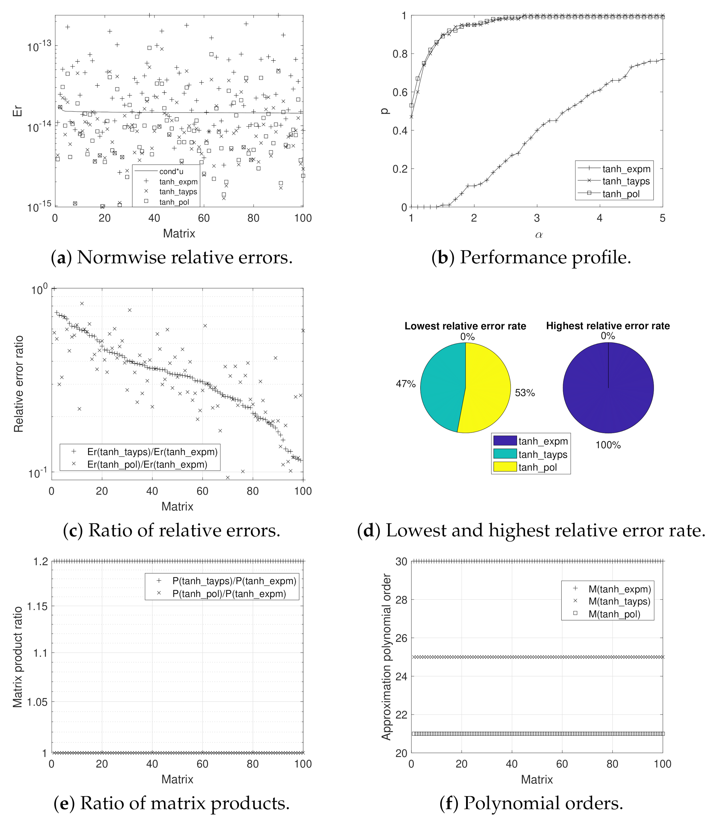
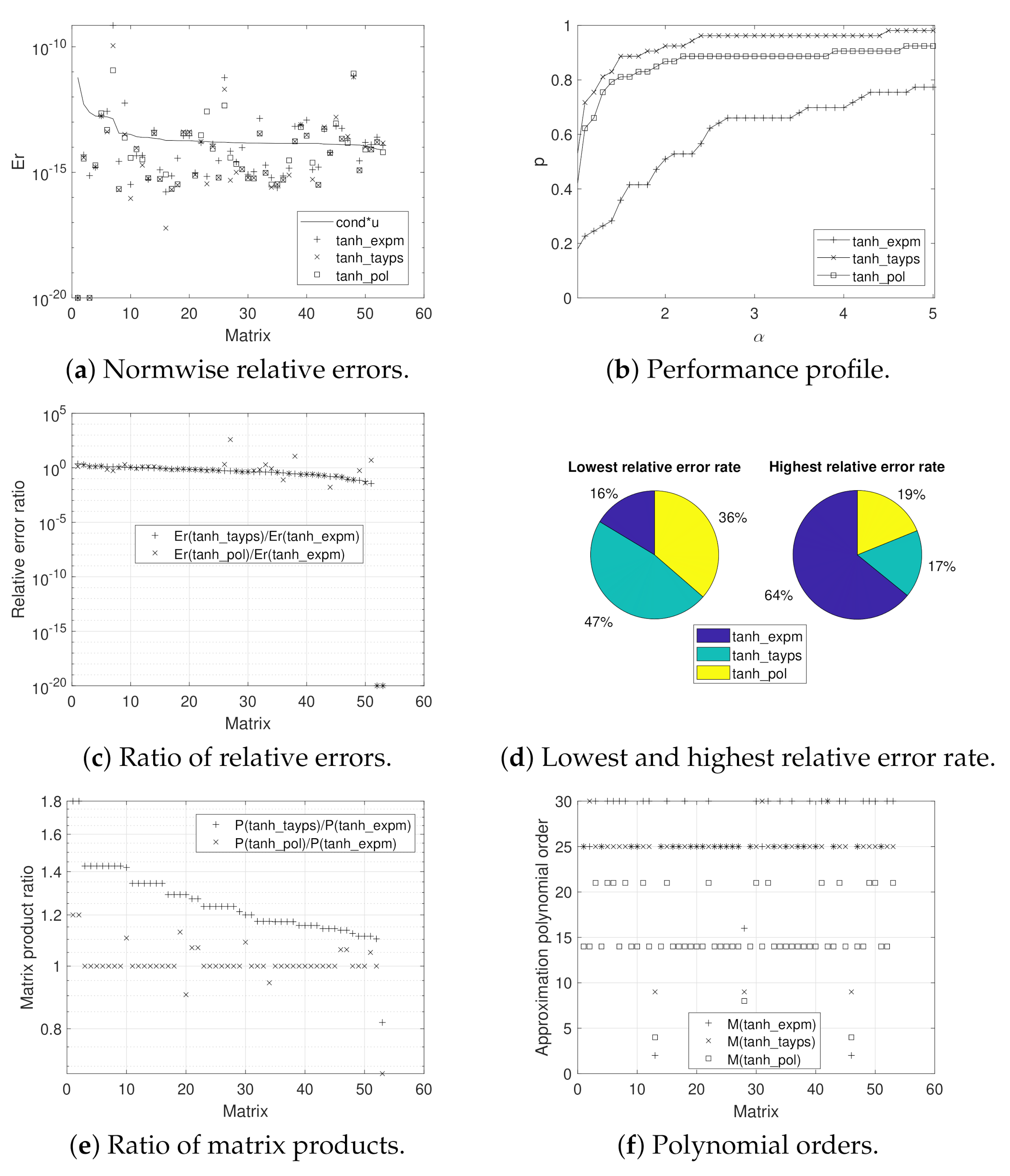
Respectively, for the three experiments, Figure 1, Figure 2 and Figure 3 illustrate the normwise relative errors (a), the performance profiles (b), the ratio of the relative errors (c), the lowest and highest relative error rate (d), the ratio of the matrix products (e), and the polynomial orders (f) for our three codes to be evaluated.
Figure 1a, Figure 2a and Figure 3a correspond to the normwise relative error. As they reveal, the three methods under evaluation were numerically stable for all the matrices that were computed, and all of them provided very accurate results, where the relative errors incurred were always less than 10 11 . The solid line that appears in these figures traces the function k tanh u , where k tanh (or c o n d ) stands for the condition number of the matrix hyperbolic tangent function [4] (Chapter 3), and u represents the unit roundoff.
It is clear that the errors incurred by all the codes were usually quite close to this line for the three experiments and even below it, as was largely the case for Tests 1 and 3. For the sake of readability in the graphs, normwise relative errors lower than 10 20 were plotted with that value in the figures. Notwithstanding, their original quantities were maintained for the rest of the results.
Figure 1b, Figure 2b and Figure 3b depict the performance profile of the codes. In them, the α coordinate on the x-axis ranges from 1 to 5 in steps equal to 0.1. For a concrete α value, the p coordinate on the y-axis indicates the probability that the considered algorithm has a relative error lower than or equal to α -times the smallest relative error over all the methods on the given test.
The implementation of tanh_tayps always achieved the results with the highest accuracy, followed closely by tanh_pol. For Tests 1 and 2, Figure 1b and Figure 2b indicate that the results provided by them are very similar, although the difference in favour of tanh_tayps is more remarkable in Test 3. As expected from the percentages given in Table 3, tanh_expm computed the hyperbolic tangent function with the worst accuracy, most notably for the matrices from Tests 2 and 3.
Precisely, the relationship among the normwise relative errors incurred by the codes to be examined is displayed in Figure 1c, Figure 2c and Figure 3c. All these ratios are presented in decreasing order with respect to Er(tanh_tayps)/Er(tanh_expm). This factor is less than 1 for the great majority of the matrices, which indicates that tanh_tayps and tanh_pol are more accurate codes than tanh_expm for estimating the hyperbolic tangent function.
These data are further corroborated by the results shown in Figure 1d, Figure 2d and Figure 3d. These graphs report the percentages of the matrices, for each of the tests, in which each code resulted in the lowest or highest normwise relative error among the errors provided by all of them. Thus, tanh_tayps exhibited the smallest relative error in 44% of the matrices for Test 1 and in 47% of them for Test 3, followed by tanh_pol in 29% and 36% of the cases, respectively. For all the other cases, tanh_expm was the most reliable method. For Test 2, tanh_pol was the most accurate code in 53% of the matrices, and tanh_tayps was the most accurate in 47% of them. In line with these results, tanh_expm was found to be the approach that led to the largest relative errors in 51% of the cases in Test 1, in 100% of them in Test 2, and in 64% for Test 3.
In contrast, although tanh_expm proved to be the most inaccurate code, it is also evident that its computational cost was usually the lowest one, as Table 4 and Figure 1e, Figure 2e and Figure 3e reported. The ratio between the number of tanh_tayps and tanh_expm matrix products ranged from 0.82 to 1.43 for Test 1, was equal to 1.20 for Test 2, and ranged from 0.82 to 1.8 for Test 3. Regarding tanh_pol and tanh_expm, this quotient varied from 0.82 to 1.13 for Test 1, from 0.68 to 1.2 for Test 3, and was equal to 1 for Test 2.
Table 5 lists, in order for Tests 1, 2, and 3, the minimum, maximum, and average values of the degree of the Taylor polynomials m and the scaling parameter s employed by the three codes. Additionally, and in a more detailed way, Figure 1f, Figure 2f and Figure 3f illustrate the order of the polynomial used in the calculation of each of the matrices that compose the testbed. The value of m allowed to be chosen was between 2 and 30 for tanh_expm and tanh_tayps and between 2 and 21 for tanh_pol. As we can see, the average value of m that was typically used varied from 25 and 30 for tanh_expm. It was around 25 for tanh_tayps, and it ranged from 14 to 21 for tanh_pol.
Having concluded the first part of the experimental results, we continue by comparing tanh_tayps and tanh_pol, the Taylor series-based codes that returned the best accuracy in the results. Table 6 presents the percentage of cases in which tanh_tayps gave place to relative errors that were lower than, greater than, or equal to those of tanh_pol. According to the exposed values, both methods provided very similar results, and the percentage of cases in which each method was more accurate than the other was approximately equal to 50% for the different tests.
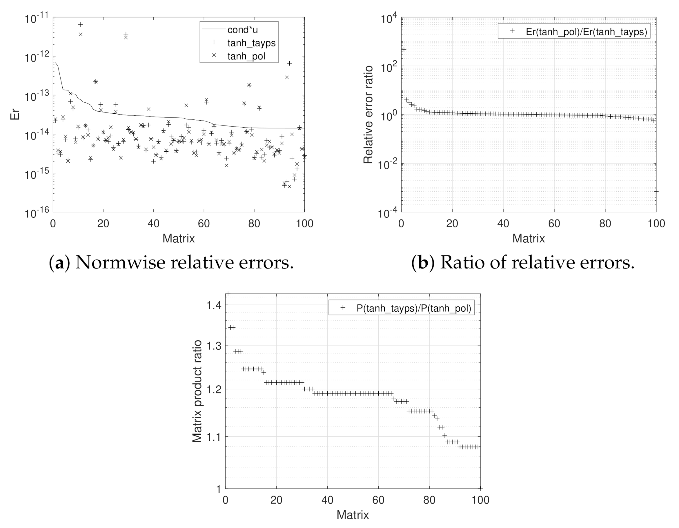
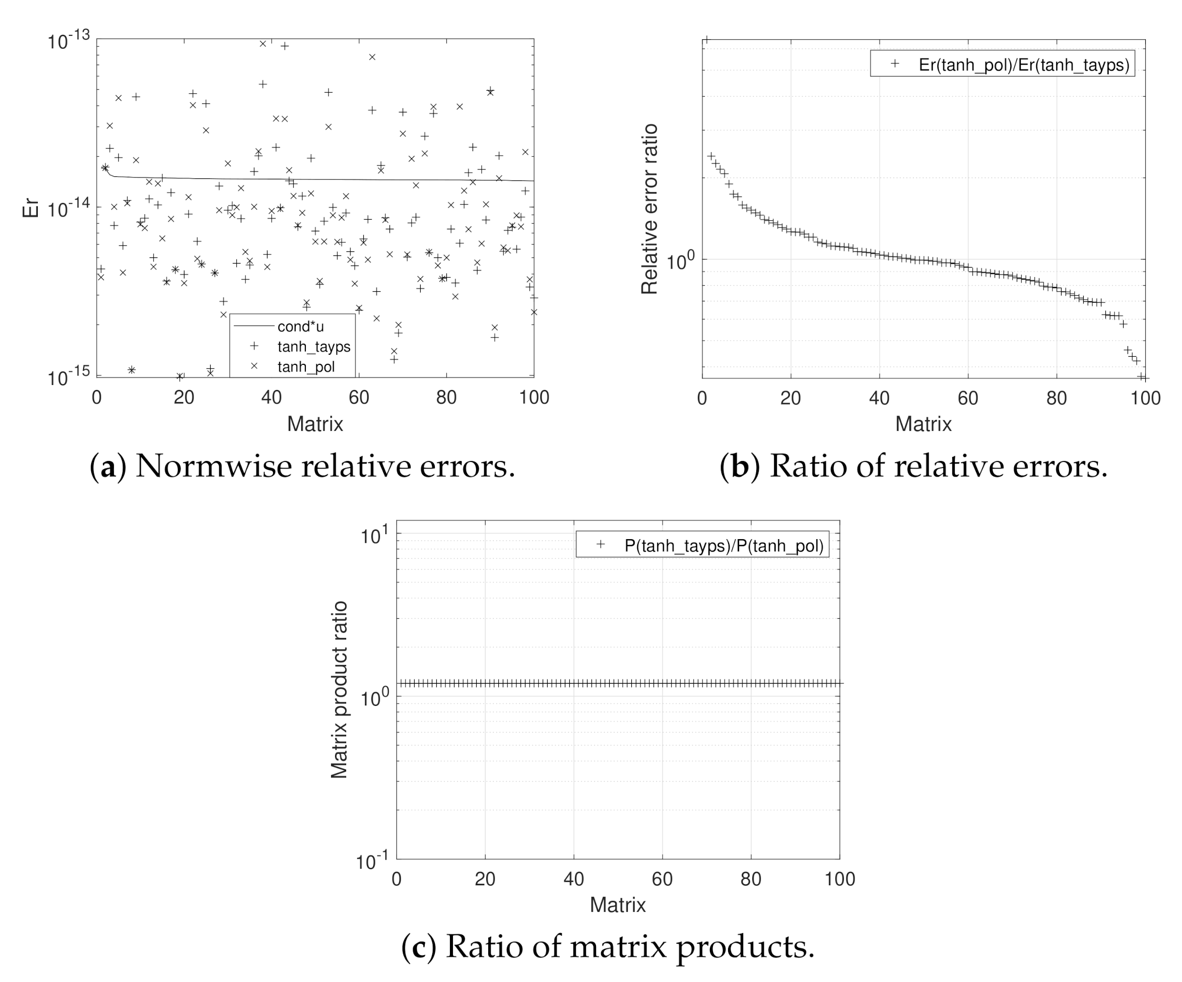
Figure 4, Figure 5 and Figure 6 incorporate the normwise relative errors (a), the ratio of relative errors (b), and the ratio of matrix products (c) between tanh_tayps and tanh_pol. The graphs corresponding to the performance profiles and the polynomial orders are not included now since the results match with those already shown in the previous figures. All this information is also complemented by Table 7, which collects, respectively for each test, the minimum, maximum, and average relative errors incurred by both methods to be analysed, together with the standard deviation.
As Table 6 details, for Tests 1 and 3, tanh_tayps slightly improved on tanh_pol in the percentage of matrices in which the relative error committed was lower, although it is true that the difference between the results provided by the two methods was small in most cases. However, when such a difference occurred, it was more often in favour of tanh_tayps than the other way around, in quantitative terms.
With all this, we can also appreciate that the mean relative error and the standard deviation incurred by tanh_pol were lower than those of tanh_tayps. For matrices that were part of Test 2, the numerical results achieved by both methods were almost identical, and the differences between them were not significant.
To conclude the analysis and with regard to the computational cost of both codes, such as depicted in Figure 4c, Figure 5c and Figure 6c, it simply remains to note that tanh_tayps performed between 1 and 1.43 more matrix products compared with tanh_pol for Test 1, 1.2 more for Test 2, and between 1.06 and 1.5 more for Test 3. Therefore, tanh_pol computed the matrix tangent function with a very similar accuracy in the results compared to tanh_tayps but with a considerably lower computational cost.

4. Conclusions

Two alternative methods to approximate the matrix hyperbolic tangent were addressed in this work. The first was derived from its own definition and reduced to the computation of a matrix exponential. The second method deals with its Taylor series expansion. In this latter approach, two alternatives were developed and differed on how the evaluation of the matrix polynomials was performed. In addition, we provided algorithms to determine the scaling factor and the order of the polynomial. As a result, we dealt with a total of three MATLAB codes (tanh_expm, tanh_tayps, and tanh_pol), which were evaluated on a complete testbed populated with matrices of three different types.
The Taylor series-based codes reached the most accurate results in the tests, a fact that is in line with the recommendation suggested in [33] of using a Taylor development against other alternatives whenever possible. However, codes based on Taylor series can be computationally expensive if the Paterson–Stockmeyer method is employed to evaluate the polynomial, as we confirmed with the tanh_tayps implementation. One idea to reduce this problem is to use Sastre formulas, as we did in our tanh_pol code, resulting in an efficient alternative that significantly reduced the number of matrix operations without affecting the accuracy.
The results found in this paper demonstrated that the three codes were stable and provided acceptable accuracy. However, and without underestimating the other two codes, the tanh_pol implementation proposed here offered the best ratio of accuracy/computational cost and proved to be an excellent method for the computation of the matrix hyperbolic tangent.

Author Contributions

Conceptualization, E.D.; methodology, E.D., J.I., J.M.A. and J.S.; software, J.I., J.M.A. and J.S.; validation, J.M.A.; formal analysis, J.I. and J.S.; investigation, E.D., J.I., J.M.A. and J.S.; writing—original draft preparation, E.D., J.I., J.M.A. and J.S.; writing—review and editing, P.A.-J. All authors have read and agreed to the published version of the manuscript.

Funding

This research was funded by the Spanish Ministerio de Ciencia e Innovación under grant number TIN2017-89314-P.

Institutional Review Board Statement

Not applicable.

Informed Consent Statement

Not applicable.

Data Availability Statement

Not applicable.

Conflicts of Interest

The authors declare no conflict of interest.

References

  1. Constantine, A.; Muirhead, R. Partial differential equations for hypergeometric functions of two argument matrices. J. Multivar. Anal. 1972, 2, 332–338. [Google Scholar] [CrossRef] [Green Version]
  2. James, A.T. Special functions of matrix and single argument in statistics. In Theory and Application of Special Functions; Academic Press: Cambridge, MA, USA, 1975; pp. 497–520. [Google Scholar]
  3. Hochbruck, M.; Ostermann, A. Exponential integrators. Acta Numer. 2010, 19, 209–286. [Google Scholar] [CrossRef] [Green Version]
  4. Higham, N.J. Functions of Matrices: Theory and Computation; Society for Industrial and Applied Mathematics: Philadelphia, PA, USA, 2008; p. 425. [Google Scholar]
  5. Rinehart, R. The Equivalence of Definitions of a Matrix Function. Am. Math. Mon. 1955, 62, 395–414. [Google Scholar] [CrossRef]
  6. Estrada, E.; Higham, D.J.; Hatano, N. Communicability and multipartite structures in complex networks at negative absolute temperatures. Phys. Rev. E 2008, 78, 026102. [Google Scholar] [CrossRef] [PubMed] [Green Version]
  7. Jódar, L.; Navarro, E.; Posso, A.; Casabán, M. Constructive solution of strongly coupled continuous hyperbolic mixed problems. Appl. Numer. Math. 2003, 47, 477–492. [Google Scholar] [CrossRef]
  8. Defez, E.; Sastre, J.; Ibáñez, J.; Peinado, J.; Tung, M.M. A method to approximate the hyperbolic sine of a matrix. Int. J. Complex Syst. Sci. 2014, 4, 41–45. [Google Scholar]
  9. Defez, E.; Sastre, J.; Ibáñez, J.; Peinado, J. Solving engineering models using hyperbolic matrix functions. Appl. Math. Model. 2016, 40, 2837–2844. [Google Scholar] [CrossRef]
  10. Defez, E.; Sastre, J.; Ibáñez, J.; Ruiz, P. Computing hyperbolic matrix functions using orthogonal matrix polynomials. In Progress in Industrial Mathematics at ECMI 2012; Springer: Berlin/Heidelberg, Germany, 2014; pp. 403–407. [Google Scholar]
  11. Defez, E.; Sastre, J.; Ibánez, J.; Peinado, J.; Tung, M.M. On the computation of the hyperbolic sine and cosine matrix functions. Model. Eng. Hum. Behav. 2013, 1, 46–59. [Google Scholar]
  12. Efimov, G.V.; Von Waldenfels, W.; Wehrse, R. Analytical solution of the non-discretized radiative transfer equation for a slab of finite optical depth. J. Quant. Spectrosc. Radiat. Transf. 1995, 53, 59–74. [Google Scholar] [CrossRef]
  13. Lehtinen, A. Analytical Treatment of Heat Sinks Cooled by Forced Convection. Ph.D. Thesis, Tampere University of Technology, Tampere, Finland, 2005. [Google Scholar]
  14. Lampio, K. Optimization of Fin Arrays Cooled by Forced or Natural Convection. Ph.D. Thesis, Tampere University of Technology, Tampere, Finland, 2018. [Google Scholar]
  15. Hilscher, R.; Zemánek, P. Trigonometric and hyperbolic systems on time scales. Dyn. Syst. Appl. 2009, 18, 483. [Google Scholar]
  16. Zemánek, P. New Results in Theory of Symplectic Systems on Time Scales. Ph.D. Thesis, Masarykova Univerzita, Brno, Czech Republic, 2011. [Google Scholar]
  17. Estrada, E.; Silver, G. Accounting for the role of long walks on networks via a new matrix function. J. Math. Anal. Appl. 2017, 449, 1581–1600. [Google Scholar] [CrossRef] [Green Version]
  18. Cieśliński, J.L. Locally exact modifications of numerical schemes. Comput. Math. Appl. 2013, 65, 1920–1938. [Google Scholar] [CrossRef]
  19. Cieśliński, J.L.; Kobus, A. Locally Exact Integrators for the Duffing Equation. Mathematics 2020, 8, 231. [Google Scholar] [CrossRef] [Green Version]
  20. Golub, G.H.; Loan, C.V. Matrix Computations, 3rd ed.; Johns Hopkins Studies in Mathematical Sciences; The Johns Hopkins University Press: Baltimore, MD, USA, 1996. [Google Scholar]
  21. Moler, C.; Van Loan, C. Nineteen Dubious Ways to Compute the Exponential of a Matrix, Twenty-Five Years Later. SIAM Rev. 2003, 45, 3–49. [Google Scholar] [CrossRef]
  22. Sastre, J.; Ibáñez, J.; Defez, E. Boosting the computation of the matrix exponential. Appl. Math. Comput. 2019, 340, 206–220. [Google Scholar] [CrossRef]
  23. Sastre, J.; Ibáñez, J.; Defez, E.; Ruiz, P. Efficient orthogonal matrix polynomial based method for computing matrix exponential. Appl. Math. Comput. 2011, 217, 6451–6463. [Google Scholar] [CrossRef] [Green Version]
  24. Sastre, J.; Ibáñez, J.; Defez, E.; Ruiz, P. New scaling-squaring Taylor algorithms for computing the matrix exponential. SIAM J. Sci. Comput. 2015, 37, A439–A455. [Google Scholar] [CrossRef]
  25. Defez, E.; Ibánez, J.; Alonso-Jordá, P.; Alonso, J.; Peinado, J. On Bernoulli matrix polynomials and matrix exponential approximation. J. Comput. Appl. Math. 2020, 113207. [Google Scholar] [CrossRef]
  26. Ruiz, P.; Sastre, J.; Ibáñez, J.; Defez, E. High perfomance computing of the matrix exponential. J. Comput. Appl. Math. 2016, 291, 370–379. [Google Scholar] [CrossRef]
  27. Paterson, M.S.; Stockmeyer, L.J. On the Number of Nonscalar Multiplications Necessary to Evaluate Polynomials. SIAM J. Comput. 1973, 2, 60–66. [Google Scholar] [CrossRef] [Green Version]
  28. Sastre, J. Efficient evaluation of matrix polynomials. Linear Algebra Appl. 2018, 539, 229–250. [Google Scholar] [CrossRef]
  29. Al-Mohy, A.H.; Higham, N.J. A New Scaling and Squaring Algorithm for the Matrix Exponential. SIAM J. Matrix Anal. Appl. 2009, 31, 970–989. [Google Scholar] [CrossRef] [Green Version]
  30. Higham, N.J. FORTRAN Codes for Estimating the One-norm of a Real or Complex Matrix, with Applications to Condition Estimation. ACM Trans. Math. Softw. 1988, 14, 381–396. [Google Scholar] [CrossRef]
  31. Higham, N.J. The Matrix Computation Toolbox. 2002. Available online: http://www.ma.man.ac.uk/~higham/mctoolbox (accessed on 7 March 2020).
  32. Wright, T.G. Eigtool, Version 2.1. 2009. Available online: http://www.comlab.ox.ac.uk/pseudospectra/eigtool (accessed on 7 March 2020).
  33. Corwell, J.; Blair, W.D. Industry Tip: Quick and Easy Matrix Exponentials. IEEE Aerosp. Electron. Syst. Mag. 2020, 35, 49–52. [Google Scholar] [CrossRef]
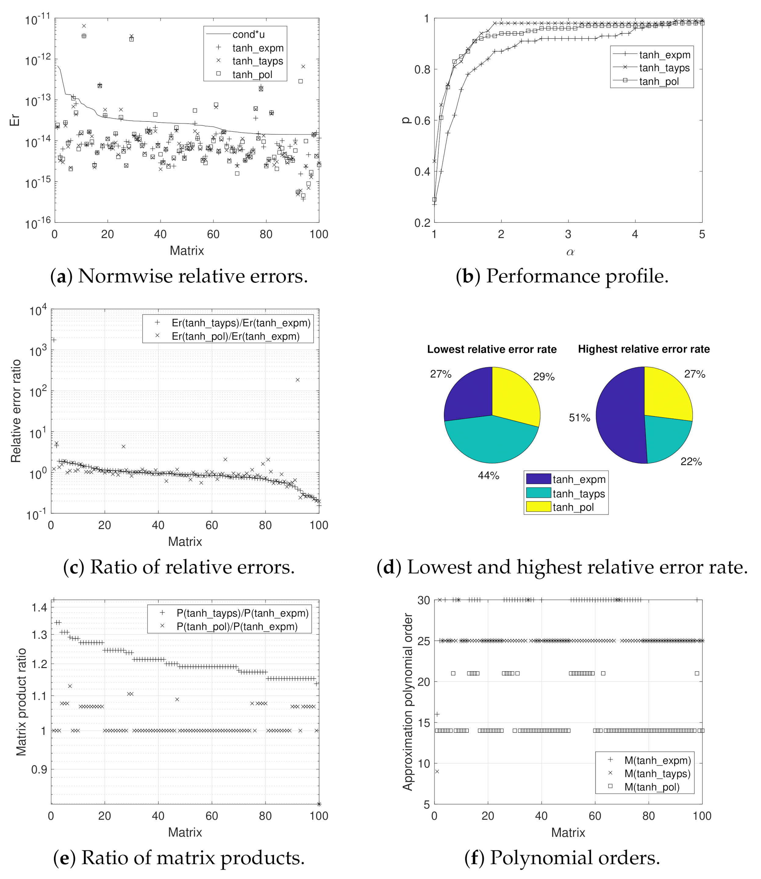
Figure 1. Experimental results for Test 1.
Mathematics 09 01219 g001
Figure 2. Experimental results for Test 2.
Mathematics 09 01219 g002
Figure 3. Experimental results for Test 3.
Mathematics 09 01219 g003
Figure 4. Experimental results for Test 1.
Mathematics 09 01219 g004
Figure 5. Experimental results for Test 2.
Mathematics 09 01219 g005
Figure 6. Experimental results for Test 3.
Mathematics 09 01219 g006
Table 1. Values of Θ m k , 1 k 9 , for polynomial evaluation by means of the Paterson–Stockmeyer method.
m 1 = 2 1.1551925093100 × 10 3
m 2 = 4 2.8530558816082 × 10 2
m 3 = 6 9.7931623314428 × 10 2
m 4 = 9 2.3519926145338 × 10 1
m 5 = 12 3.7089935615781 × 10 1
m 6 = 16 5.2612365603423 × 10 1
m 7 = 20 6.5111831924355 × 10 1
m 8 = 25 7.73638541973549 × 10 1
m 9 = 30 8.68708923627294 × 10 1
Table 2. Values of Θ m k , 1 k 5 , for polynomial evaluation using the Sastre formulas.
m 1 = 2 1.1551925093100 × 10 3
m 2 = 4 2.8530558816082 × 10 2
m 3 = 8 1.88126704493647 × 10 1
m 4 = 14 + 4.65700446893510 × 10 1
m 5 = 21 + 6.84669656651721 × 10 1
Table 3. The relative error comparison, for the three tests, between tanh_expm vs. tanh_tayps and tanh_expm vs tanh_pol.
Test 1Test 2Test 3
Er(tanh_expm)<Er(tanh_tayps)32%0%22.64%
Er(tanh_expm)>Er(tanh_tayps)68%100%77.36%
Er(tanh_expm)=Er(tanh_tayps)0%0%0%
Er(tanh_expm)<Er(tanh_pol)44%0%30.19%
Er(tanh_expm)>Er(tanh_pol)56%100%69.81%
Er(tanh_expm)=Er(tanh_pol)0%0%0%
Table 4. Matrix products (P) corresponding to the tanh_expm, tanh_tayps, and tanh_pol functions for Tests 1–3.
Test 1Test 2Test 3
P(tanh_expm)18101500848
P(tanh_tayps)218018001030
P(tanh_pol)18471500855
Table 5. The minimum, maximum, and average parameters m and s employed for Tests 1–3, respectively.
m s
Min.Max.AverageMin.Max.Average
tanh_expm163027.41053.55
tanh_tayps93025.09064.65
tanh_pol142115.47064.83
tanh_expm303030.00222.00
tanh_tayps252525.00333.00
tanh_pol212121.00333.00
tanh_expm23026.23082.77
tanh_tayps93024.38093.74
tanh_pol42115.36093.87
Table 6. The relative error comparison for the three tests between tanh_tayps vs. tanh_pol.
Test 1Test 2Test 3
Er(tanh_tayps)<Er(tanh_pol)56%47%50.94%
Er(tanh_tayps)>Er(tanh_pol)44%53%45.28%
Er(tanh_tayps)=Er(tanh_pol)0%0%3.77%
Table 7. The minimum, maximum, and average values and the standard deviation of the relative errors committed by tanh_tayps and tanh_pol for Tests 1–3.
MinimumMaximumAverageStandard Deviation
tanh_tayps 4.84 × 10 16 6.45 × 10 12 1.22 × 10 13 7.40 × 10 13
tanh_pol 4.55 × 10 16 3.64 × 10 12 8.48 × 10 14 4.69 × 10 13
tanh_tayps 9.71 × 10 16 9.06 × 10 14 1.25 × 10 14 1.41 × 10 14
tanh_pol 9.92 × 10 16 9.35 × 10 14 1.26 × 10 14 1.47 × 10 14
tanh_tayps 1.09 × 10 254 1.10 × 10 10 2.26 × 10 12 1.52 × 10 11
tanh_pol 1.09 × 10 254 1.16 × 10 11 4.10 × 10 13 1.96 × 10 12
Publisher’s Note: MDPI stays neutral with regard to jurisdictional claims in published maps and institutional affiliations.