
Cliques Are Bricks for k-CT Graphs


Abstract
1. Introduction
2. Terminology and Notation
3. Composition of k—CT Graphs from Cliques
- 1.
- if and , then ,
- 2.
- for every .
3.1. Closed Trail Distance in an Undirected Graph
3.2. Construction of Graphs
- when ,
- when ,
- when .
- 1.
- for ,
- 2.
- for ,
- 3.
- for and .
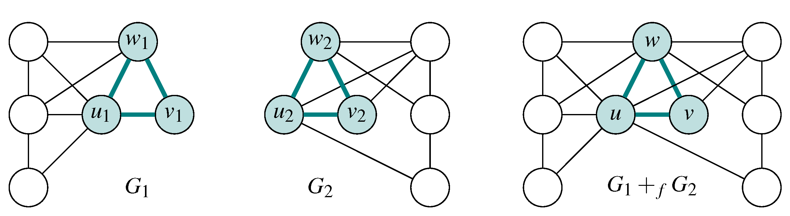
- According to Lemma 1 , , , and . We consider the following situations in the glued graph :
- (a)
- if , then ;
- (b)
- if both vertices or , then ;
- (c)
- if , , and is glued with via v, then .
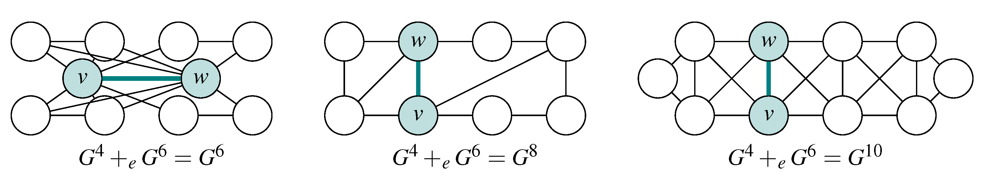
From these situations, it follows that . - The gluing occurs via the edge , where and .
- (a)
- If or , then .
- (b)
- If both vertices or , then .
- (c)
- If and , then exists for all , and exists for all , . From the existence of two cycles with lengths equal to three that share a common edge follows the existence of , where the edge is the chord of cycle and .
From these situations, it follows that . - The proof is similar to the previous situation where the graphs are glued via with .
- (a)
- If both vertices , then .
- (b)
- If both vertices or , then .
- (c)
- If and , then, where .
From these situations, it follows that .
- 1.
- for ,
- 2.
- for ,
- 3.
- for , and
- 4.
- for .
- It follows from Definition 3 of k-CT graphs that the CT distance between two different vertices of the cycle is k and . The cycle is the sparsest k-CT graph.
- When we glue and cycle graphs so that they share one vertex v, then, from the properties of the cycles, it follows that: , and , . The CT distance in the glued graph is for all vertices in and for all vertices in . Therefore, .
- When we glue the and cycles so that they share one edge , the resulting graph is a cycle with the chord e, and it has vertices. The CT distance is for all vertices in , where , and for all vertices in , where . Other CT distances in the glued graph are smaller than , and the glued graph is from the set .
- When we glue the clique and cycle so that they share one edge , then the resulting graph contains cycles with chord e and vertices. The CT distance is for all vertices in , where , and for all vertices in , where . Other CT distances in the glued graph are smaller than , and the glued graph is from the set .
- If , then;
- If , thenconsists of or , the edge e, and the rest of or . In this situation: where .
- 1.
- , where for and for ;
- 2.
- , where for and for .
- The lower estimate of r:
- (a)
- Proof by contradiction. Let for and . There exist and , such that and . From the assumption, it follows that , which is in contradiction with the CT distance between and , which is longer than or equal to 6, which follows from Theorem 2 part 1.
- (b)
- It is obvious that for , is true.
The upper estimate of r follows from Theorem 3 part 2. - The lower estimate of r:
- (a)
- It is obvious that for . It follows from Theorem 2 part 2.
- (b)
- The situation with is obvious. The CT distance in a glued graph cannot be shorter than the CT distance in the part of the glued graph.
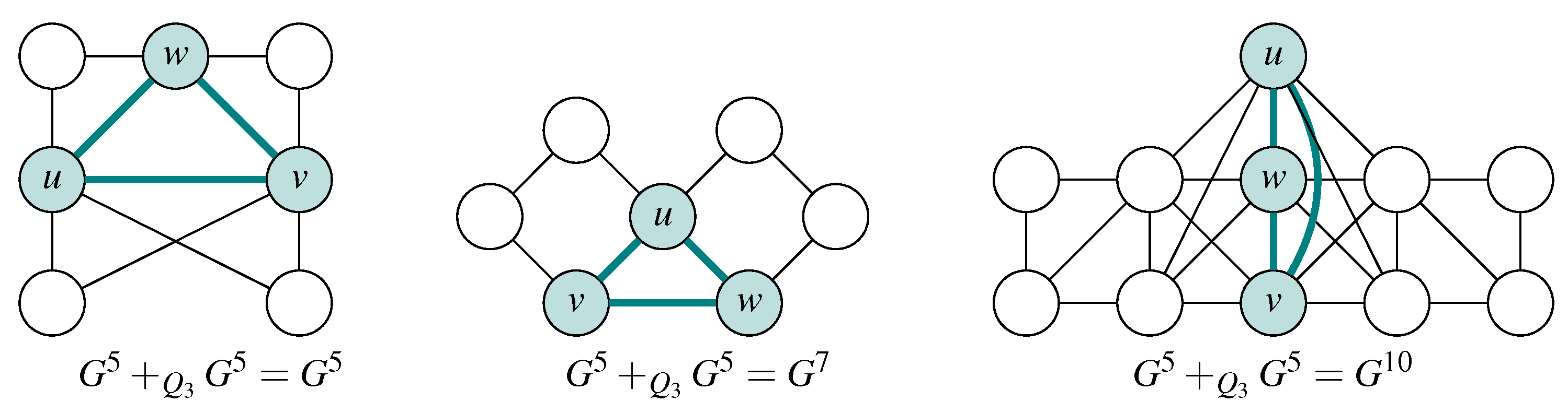
The upper estimate of r follows from Lemma 3 and Theorem 3 part 3. An example of this situation is shown by the last image in Figure 5.
- 1.
- , where for each ;
- 2.
- , where for each [( and ) or ( and )].
- The lower estimate of r: A glued graph via the vertex v has the vertex v as an articulation. From Lemma 4, it follows that the with cannot contain articulation. The smallest r for the glued graph via the vertex v is 6. The upper estimate of r follows from Theorem 3 part 2.
- The lower estimate of r: From Definition 3 and Definition 6, it follows that it is impossible to obtain a glued graph with and . The upper estimate of r follows from Theorem 3 part 2.
4. Conclusions
Author Contributions
Funding
Institutional Review Board Statement
Informed Consent Statement
Data Availability Statement
Conflicts of Interest
References
- Yin, H.; Benson, A.R.; Leskovec, J. Higher-order clustering in networks. Phys. Rev. E 2018, 97, 052306. [Google Scholar] [CrossRef] [PubMed]
- Prokop, P.; Snášel, V.; Dráždilová, P.; Platoš, J. Clustering and Closure Coefficient Based on k–CT Components. IEEE Access 2020, 8, 101145–101152. [Google Scholar] [CrossRef]
- Torres, L.; Blevins, A.S.; Bassett, D.S.; Eliassi-Rad, T. The why, how, and when of representations for complex systems. arXiv 2020, arXiv:2006.02870. [Google Scholar]
- Iacopini, I.; Petri, G.; Barrat, A.; Latora, V. Simplicial models of social contagion. Nat. Commun. 2019, 10, 2485. [Google Scholar] [CrossRef]
- Xia, K.; Wei, G.W. A review of geometric, topological and graph theory apparatuses for the modeling and analysis of biomolecular data. arXiv 2016, arXiv:1612.01735. [Google Scholar]
- Snášel, V.; Nowaková, J.; Xhafa, F.; Barolli, L. Geometrical and topological approaches to Big Data. Future Gener. Comput. Syst. 2017, 67, 286–296. [Google Scholar] [CrossRef]
- Serrano, D.H.; Gómez, D.S. Centrality measures in simplicial complexes: Applications of topological data analysis to network science. Appl. Math. Comput. 2020, 382, 125331. [Google Scholar]
- Leskovec, J.; Lang, K.J.; Dasgupta, A.; Mahoney, M.W. Community structure in large networks: Natural cluster sizes and the absence of large well-defined clusters. Internet Math. 2009, 6, 29–123. [Google Scholar] [CrossRef]
- Borůvka, O. O jistém problému minimálním [About a certain minimal problem]. In Práce Moravské Přírodovědecké Společnosti v Brně III; 1926; pp. 37–58. Available online: http://hdl.handle.net/10338.dmlcz/500114 (accessed on 20 May 2021).
- Nešetřil, J.; Milková, E.; Nešetřilová, H. Otakar Borůvka on minimum spanning tree problem translation of both the 1926 papers, comments, history. Discret. Math. 2001, 233, 3–36. [Google Scholar] [CrossRef]
- Carlsson, G. Topology and data. Bull. Am. Math. Soc. 2009, 46, 255–308. [Google Scholar] [CrossRef]
- Carlsson, G. Topological pattern recognition for point cloud data. Acta Numer. 2014, 23, 289. [Google Scholar] [CrossRef]
- De Silva, V.; Ghrist, R. Homological sensor networks. Not. Am. Math. Soc. 2007, 54, 10–17. [Google Scholar]
- De Silva, V.; Ghrist, R.; Muhammad, A. Blind Swarms for Coverage in 2D. In Proceedings of the Robotics: Science and Systems 2005, Cambridge, MA, USA, 8–11 June 2005; pp. 335–342. [Google Scholar]
- Schwerdtfeger, P.; Wirz, L.N.; Avery, J. The topology of fullerenes. Wiley Interdiscip. Rev. Comput. Mol. Sci. 2015, 5, 96–145. [Google Scholar] [CrossRef]
- Vázquez, A.; Oliveira, J.G.; Barabási, A.L. In homogeneous evolution of subgraphs and cycles in complex networks. Phys. Rev. E 2005, 71, 025103. [Google Scholar] [CrossRef] [PubMed]
- Ashrafi, A.R.; Diudea, M.V. Distance, Symmetry, and Topology in Carbon Nanomaterials; Springer: Cham, Switzerland, 2016; Volume 9. [Google Scholar]
- Goddard, W.; Oellermann, O.R. Distance in graphs. In Structural Analysis of Complex Networks; Springer: Cham, Switzerland, 2011; pp. 49–72. [Google Scholar]
- Chebotarev, P. The walk distances in graphs. Discret. Appl. Math. 2012, 160, 1484–1500. [Google Scholar] [CrossRef]
- Deza, M.M.; Deza, E. Encyclopedia of distances. In Encyclopedia of Distances; Springer: Cham, Switzerland, 2009; pp. 1–583. [Google Scholar]
- Estrada, E. The communicability distance in graphs. Linear Algebra Its Appl. 2012, 436, 4317–4328. [Google Scholar] [CrossRef]
- Luxburg, U.V.; Radl, A.; Hein, M. Getting lost in space: Large sample analysis of the resistance distance. Adv. Neural Inf. Process. Syst. 2010, 23, 2622–2630. [Google Scholar]
- Snášel, V.; Dráždilová, P.; Platoš, J. Closed trail distance in a biconnected graph. PLoS ONE 2018, 13, e0202181. [Google Scholar] [CrossRef]
- Gross, J.L.; Yellen, J. Handbook of Graph Theory; CRC Press: Abingdon, UK, 2004; p. 1155. [Google Scholar]
- Scoville, N.A. Discrete Morse Theory; American Mathematical Soc.: Providence, RI, USA, 2019; Volume 90. [Google Scholar]
- Nešetřil, J. Amalgamation of graphs and its application. Ann. N. Y. Acad. Sci. 2006, 319, 415–428. [Google Scholar] [CrossRef]
- Heckel, R.; Taentzer, G. Graph Transformation, Specifications, and Nets; Springer: Cham, Switzerland, 2018. [Google Scholar]
- Pimpasalee, W.; Uiyyasathian, C. Clique Coverings of Glued Graphs at Complete Clones. Int. Math. Forum 2010, 5, 1155–1166. [Google Scholar]
- Lovász, L. Graph minor theory. Bull. Am. Math. Soc. 2006, 43, 75–86. [Google Scholar] [CrossRef]


Publisher’s Note: MDPI stays neutral with regard to jurisdictional claims in published maps and institutional affiliations. |
© 2021 by the authors. Licensee MDPI, Basel, Switzerland. This article is an open access article distributed under the terms and conditions of the Creative Commons Attribution (CC BY) license (https://creativecommons.org/licenses/by/4.0/).
Share and Cite
Snášel, V.; Dráždilová, P.; Platoš, J. Cliques Are Bricks for k-CT Graphs. Mathematics 2021, 9, 1160. https://doi.org/10.3390/math9111160
Snášel V, Dráždilová P, Platoš J. Cliques Are Bricks for k-CT Graphs. Mathematics. 2021; 9(11):1160. https://doi.org/10.3390/math9111160
Chicago/Turabian StyleSnášel, Václav, Pavla Dráždilová, and Jan Platoš. 2021. "Cliques Are Bricks for k-CT Graphs" Mathematics 9, no. 11: 1160. https://doi.org/10.3390/math9111160
APA StyleSnášel, V., Dráždilová, P., & Platoš, J. (2021). Cliques Are Bricks for k-CT Graphs. Mathematics, 9(11), 1160. https://doi.org/10.3390/math9111160