Hermite Interpolation Based Interval Shannon-Cosine Wavelet and Its Application in Sparse Representation of Curve

Abstract

Using the wavelet transform defined in the infinite domain to process the signal defined in finite interval, the wavelet transform coefficients at the boundary are usually very large. It will bring severe boundary effect, which reduces the calculation accuracy. The construction of interval wavelet is the most common method to reduce the boundary effect. By studying the properties of Shannon-Cosine interpolation wavelet, an improved version of the wavelet function is proposed, and the corresponding interval interpolation wavelet based on Hermite interpolation extension and variational principle is designed, which possesses almost all of the excellent properties such as interpolation, smoothness, compact support and normalization. Then, the multi-scale interpolation operator is constructed, which can be applied to select the sparse feature points and reconstruct signal based on these sparse points adaptively. To validate the effectiveness of the proposed method, we compare the proposed method with Shannon-Cosine interpolation wavelet method, Akima method, Bezier method and cubic spline method by taking infinitesimal derivable function $cos\left(x\right)$ and irregular piecewise function as an example. In the reconstruction of $cos\left(x\right)$ and piecewise function, the proposed method reduces the boundary effect at the endpoints. When the interpolation points are the same, the maximum error, average absolute error, mean square error and running time are $1.20$ × 10${}^{-4}$, $2.52$ × 10${}^{-3}$, $2.76$ × 10${}^{-5}$, $1.68$ × 10${}^{-2}$ and $4.02$ × 10${}^{-3}$, $4.94$ × 10${}^{-4}$, $1.11$ × 10${}^{-3}$, $9.27$ × 10${}^{-3}$, respectively. The four indicators mentioned above are all lower than the other three methods. When reconstructing an infinitely derivable function, the curve reconstructed by our method is smoother, and it satisfies $C^2$ and $G^2$ continuity. Therefore, the proposed method can better realize the reconstruction of smooth curves, improve the reconstruction efficiency and provide new ideas to the curve reconstruction method.

1. Introduction

In modern industrial manufacturing technology, curve and surface modeling technology is one of the very important technologies, and its plays an important role in numerical fitting and approximation; computer vision; streamlined design of crafts, outline design of aircraft, automobiles and ships; restoration of cultural relics; geological surface interpolation [1]; reverse engineering [2,3]; and other fields. Besides, it is the core of computer-aided geometric design (CAGD) [4].

In practical applications, interpolation techniques [5,6] are often used to reconstruct signals accurately on some interpolation points. The common interpolation methods include Bezier method [7], B-Spline method [8,9] and non-uniform rational B-Spline (NURBS) method [10,11]. Some other methods are based on these classical methods: interpolation basis function method [12,13], interpolation geometry iteration method [14], interpolation subdivision method [15], etc. The subdivision method is applicable for any topology structure, but unfortunately it is difficult to obtain the analytical expression of the curve. Subdivision method is a subdivision iterative process from coarse to fine. This process generates a multi-level sequence of the model, that is, the model is transformed from low resolution to high resolution, which is similar to multi-resolution analysis [16,17]. In fact, wavelet analysis is an important way to realize multi-resolution analysis. There have been many studies using wavelet analysis theory [18,19] with interpolation characteristics for approximation of different smoothness curves, which have made effective progress in effectively suppressing the boundary effect brought by wavelet transform and further in improving the approximation accuracy.

Shannon-Cosine wavelet [20,21,22] has been proposed recently, it not only has excellent properties such as normalization, interpolation, double scale, compact support, smoothness and analytical expression, but also the support interval and smoothness of wavelet function can be controlled through iterative parameters adaptively. The excellence of Shannon-Cosine interpolation wavelet has been verified in the solution of fractional partial differential equations [20].

However, wavelet transform is defined on an infinite interval and the signals are defined on a finite interval; direct use of wavelet transform will produce a large-scale boundary effect [23,24]. Constructing interval wavelet is the most common method to solve the boundary effect. Interval wavelet based on generalized variational principle is constructed based on boundary extension, that is, the extension is mapped into wavelet function by generalized variational principle. Common extension methods [25,26] include symmetric extension [27,28], zero extension [29], periodic extension and mirror extension [30]. Each method has its applicable scope, for example, periodic extension is only suitable for periodic functions and mirror extension is only suitable for signals with Neumman boundary conditions.

There exist several common methods for constructing interval interpolation wavelets on bounded intervals, such as extrapolation [31], spline interpolation [32,33,34], Newton interpolation, polynomial method [35,36,37] and central affine change method. Lagrange extrapolation method [38] is the most commonly used method for constructing interval wavelets. However, when the gradient of approximation function is large, interpolation points need to be added, and the resulting Gibbs phenomenon [39] will also cause errors. Chebyshev-polynomial wavelets [35] require weights in their scalar products, which may lead to difficulties in balancing the relative significance of their coefficients. Mei et al. [24] constructed a dynamic interval wavelet based on the Newton interpolation method, which can dynamically select the extrapolation points in the interval wavelet and limit the boundary effect without increasing calculation amount. Bin and Michelle [28] constructed a interval wavelet based on symmetry on interval $[0,1]$. Wei et al. [40,41] constructed the interval wavelet based on central affine transformation extension method. This extension method ensures smooth and continuous at the extension boundary, and the smoothness of the extension function in the extension interval is consistent with the original signal. However, it does not decay to zero in the extension interval and the signal boundary may also contain high-frequency signals, which is equivalent to moving the boundary effect in the effective interval into the extension interval. To avoid the boundary effect from backing to the effective interval of the signal again, the extension interval scope needs to be increased, which leads to a large increase in calculation amount and a decrease in efficiency. Therefore, our paper constructs an interval wavelet based on Hermite interpolation, so that it attenuates to zero in the extension interval, and essentially reduces the influence of boundary effects.

The purpose of this research is to construct a novel algorithm for the reconstruction of curves by the means of the Shannon-Cosine interpolation wavelet and Hermite interpolation extension. In this scheme, the Shannon-Cosine interpolation wavelet possesses many excellent numerical properties such as the interpolation, the compact support, symmetry, smoothness analytical expression and so on. The Hermite interpolation extension can eliminate the boundary effect as it is smooth in the interval $[-\infty ,\infty ]$. This paper is organized as follows. We review the properties of Shannon-Cosine wavelet first. Then, we construct the interval Shannon-Cosine interpolation wavelet based on Hermite interpolation and variational principle. Third, we design a multi-scale interpolation operator based on interval Shannon-Cosine interpolation wavelet and some properties are proved. Finally, we perform some numerical examples in reconstructing curves.

2. Shannon-Cosine Interpolation Wavelet

Shannon-like wavelet possesses almost all the excellent numerical properties such as interpolation, smoothness, continuity, orthogonality, fast calculation speed and infinite differentiability, except the compact support domain, which limits its applications greatly.

To make use of the excellent properties of Shannon wavelet, researchers proposed many methods to improve it. The methods are usually used to improve the compact support by introducing windows functions [42,43], such as Meyer window [44], Nuttall window, Blackman window [45], Gauss window [46,47], etc. Similar to windowed Fourier transform, windowing function accelerates the delay speed of Shannon wavelet function, but it also destroys the normalization characteristic of Shannon function. Hoffman and Wei constructed Shannon–Gabor wavelet [48] by introducing Gauss window to Shannon wavelet, which is called quasi-wavelet because it does not satisfy compact support characteristic and normalization characteristic. When approximating the signal, the original signal will be amplified or reduced, which leads to the limited application scope of Shannon–Gabor wavelet. Therefore, windowing is not recommended [20,21].

To satisfy the normalization condition and improve the compact support of Shannon wavelet, we take the linear combination of the cosine functions instead of Gaussian to improve the compact support property Shannon. The Shannon-Cosine wavelet scale function used in this paper can be expressed as follows

$$S_c\left(x\right)={\displaystyle \frac{sin\left(\pi x\right)}{\pi x}}{T}_N^m\left(x\right)R_N\left(x\right)$$

(1)

where

$$T_N^m\left(x\right)={\displaystyle \frac{1}{2^{m-1}}}{\left(cos\left({\displaystyle \frac{\pi x}{N}}\right)\right)}^{2m}$$

(2)

$$R_N\left(x\right)=\chi (x+{\displaystyle \frac{N}{2}})-\chi (x-{\displaystyle \frac{N}{2}})$$

(3)

where $R_N\left(x\right)$ is a rectangular pulse function on the interval $[-{\displaystyle \frac{N}{2}},{\displaystyle \frac{N}{2}}]$, N is a constant related to the support interval, $S_c\left(x\right)$ is a Shannon-Cosine wavelet function, $T_N^m\left(x\right)$ is a linear combination of cosine functions, $a_n$ is a linear combination coefficient controlling the smoothness of the function and $\chi \left(x\right)$ is a Heaviside function, defined as follows

$$\chi \left(x\right)=\left\{\begin{array}{cc}0,\hfill & \mathrm{x}<0\hfill \\ {\displaystyle \frac{1}{2}}\hfill & \mathrm{x}=0\hfill \\ 1,\hfill & \mathrm{x}>0\hfill \end{array}\right.$$

(4)

It should be pointed out that the Shannon-Cosine wavelet function is different from one proposed in Reference [20], in which the parameter $a_n$ should be used to control the smoothness of $S_c\left(x\right)$. $S_c\left(x\right)$ in Reference [20] is a continuous differentiable function in the interval $\left(-{\displaystyle \frac{N}{2}},{\displaystyle \frac{N}{2}}\right)$, but it is not always continuous at the endpoints of the interval. To satisfy the continuity at the end points $x=\pm N/2$, let

$$\frac{{\mathrm{d}}^n}{\mathrm{d}{x}^n}{S}_c\left(x\right)\left|{}_{x=\frac{N}{2}}\right.=0,n=0,1,\dots ,m+1$$

(5)

Since $\sin \mathrm{c}\left(x\right)$ is infinitely differentiable, $R_N\left(x\right)$ is just a truncated function, and Equation (5) is equivalent to the following equation

$$\frac{{\mathrm{d}}^n}{\mathrm{d}{x}^n}{T}_N^m\left(x\right)\left|{}_{x=\frac{N}{2}}\right.=0,n=0,1,\dots ,m+1$$

(6)

As an interpolation function, it satisfies

$$S_c\left(0\right)=1$$

(7)

Substituting $x=N/2$ (or $x=-N/2$) and $x=0$ into Equations (1) and (6), we can get the linear algebraic equations about parameter $a_i(i=0,1,\cdots ,m)$. Mei and Gao [20] gave the recurrence formula of $a_n$ in detail

$$a_n=\frac{{(-1)}^n{\displaystyle \prod _{i=1}^{n-1}}{i}^2{a}_0-{\displaystyle \sum _{k=n+1}^m}\left({(-1)}^k{\displaystyle \prod _{i=1}^{n-1}}(k^2-i^2)a_k\right)}{{(-1)}^n{\displaystyle \prod _{i=1}^{n-1}}(n^2-i^2)}$$

(8)

where $a_0$ can be obtained by solving equation ${\displaystyle \sum _{i=0}^m}{a}_i=1$, and the value of $a_i(i=1,2,\dots )$ is related to the value of m, which is given in

Table 1. Value of $a_i$$(i=i,2,\dots$).

m	${\mathit{a}}_0$	${\mathit{a}}_1$	${\mathit{a}}_2$	${\mathit{a}}_3$	${\mathit{a}}_4$	${\mathit{a}}_5$	${\mathit{a}}_6$	${\mathit{a}}_7$
000	1
100	1/2	1/2
200	3/8	1/2	1/8
300	5/16	15/32	3/16	1/32
400	35/128	7/16	7/32	1/16	1/128
500	63/256	105/256	15/64	45/512	5/256	1/512
600	231/1024	99/256	495/2048	55/512	33/1024	3/512	1/2048
700	429/2048	3003/8192	1001/4096	1001/8192	91/2048	91/8192	7/4096	1/8192

.

It is obvious that the wavelet function $S_c\left(x\right)$ is equvilent with one proposed in Reference [20] as the parameter $m\le 3$. Generally, when $m=3$, the smoothness of the curve can be guaranteed. We select $m=3$ in our experiment.

Theorem 1.

The Shannon-Cosine wavelet scaling function (1) (as shown in Equations (1)) is a smooth function in the tight support interval $\left[-{\displaystyle \frac{N}{2}},{\displaystyle \frac{N}{2}}\right]$.

Proof of Theorem 1.

According to the definition of the smooth function, which refers to an infinitely differentiable function, we only need to prove that $S_c\left(x\right)$ is infinitely differentiable.

Let $f\left(x\right)={\displaystyle \frac{sin\left(\pi x\right)}{\pi x}}$, $g\left(x\right)={\displaystyle \frac{1}{2^{m-1}}}{\left(cos\left({\displaystyle \frac{\pi x}{N}}\right)\right)}^{2m}$. Obviously, $f\left(x\right)$ and $g\left(x\right)$ are infinitely differentiable functions.

In the interval $\left(-\frac{N}{2},\frac{N}{2}\right)$, $R_N\left(x\right)=1$. $S_c\left(x\right)$ can be described as

$$S_c\left(x\right)={\displaystyle \frac{sin\left(\pi x\right)}{\pi x}}{\displaystyle \frac{1}{2^{m-1}}}{\left(cos\left({\displaystyle \frac{\pi x}{N}}\right)\right)}^{2m}$$

(9)

According to the definition of Leibniz formula, we know that

$$\begin{array}{ccc}\hfill & {(f\left(x\right)\pm g\left(x\right))}^{\left(n\right)}=f{\left(x\right)}^{\left(n\right)}\pm g{\left(x\right)}^{\left(n\right)}\hfill & \\ \hfill & {\left(f\left(x\right)g\left(x\right)\right)}^{\left(n\right)}=\sum _{k=0}^{\left(n\right)}{C}_n^{k}f{\left(x\right)}^{(n-k)}g{\left(x\right)}^{\left(k\right)}\hfill & \end{array}$$

(10)

where, $C_n^k={\displaystyle \frac{n!}{k!(n-k)!}}$, $u^{\left(0\right)}=u$, $v^{\left(0\right)}=v$.

It can be proved that $S_c\left(x\right)$ is a smooth function in the interval $\left(-{\displaystyle \frac{N}{2}},{\displaystyle \frac{N}{2}}\right)$.

Then, we prove the continuity of the functions $S_c\left(x\right)$ at the endpoints $x=\pm N/2$. To the Equation (2) proposed in this paper is obvious. To the function $S_c\left(x\right)$ in Reference [20], we also give its proof as follows.

It is known that when m = 3, $a_0={\displaystyle \frac{5}{16}}$, $a_1={\displaystyle \frac{15}{32}}$, $a_2={\displaystyle \frac{3}{16}}$, $a_3={\displaystyle \frac{1}{32}}$. $S_c\left(x\right)$ can be described as

$$S_c\left(x\right)={\displaystyle \frac{sin\left(\pi x\right)}{\pi x}}\left({\displaystyle \frac{5}{16}}cos0+{\displaystyle \frac{15}{32}}cos{\displaystyle \frac{2\pi x}{N}}+{\displaystyle \frac{3}{16}}cos{\displaystyle \frac{4\pi x}{N}}+{\displaystyle \frac{1}{32}}cos{\displaystyle \frac{6\pi x}{N}}\right)R_N\left(x\right)$$

(11)

When $x=N/2$, $S_c\left({\displaystyle \frac{N}{2}}\right)=0\times {\displaystyle \frac{1}{2}}=0$.

When $x\to N/2^{-}$, ${lim}_{x\to N/2^{-}}{S}_c\left(x\right)=0\times 1=0=S_c\left({\displaystyle \frac{N}{2}}\right)$.

Thus, $S_c\left(x\right)$ is continuous at $x=N/2$, and similarly we can prove that $S_c\left(x\right)$ is continuous at $x=-N/2$. It can be proved that $S_c\left(x\right)$ is a smooth function in the support interval $\left[-{\displaystyle \frac{N}{2}},{\displaystyle \frac{N}{2}}\right]$.

This completes the proof. □

Figure 1 is a comparison between Shannon scale function and Shannon-Cosine interpolation wavelet scale function. We can see from the diagram that Shannon-Cosine interpolation wavelet is a real compact support function, not a quasi-wavelet as Shannon–Gabor.

3. Construction of Interval Shannon-Cosine Interpolation Wavelet Based on Hermite Interpolation Extension

The wavelet transform is defined by convolution operation and the wavelet basis function appears as a smooth function. When the signal and the wavelet function perform a convolution operation, if the end of the signal is not zero, then one side has a value and the other side is zero in the support interval of the wavelet, which will produce high frequency information and cause boundary effect. In this paper, we construct interval interpolation wavelet based on Hermite interpolation extension and variational principle. We assume that the first-order derivative value and function value at the left end of the extension interval are all zero, and the first-order derivative value and the function value at the right end of the extension interval are equal to the function value and first-order derivative value of the signal. Then, a smooth function is obtained by using two-point cubic piecewise Hermite interpolation, which can keep the signals in the extension interval and the effective interval smooth and continuous at the boundary and decay to zero smoothly in the extension interval, thus the boundary effect is reduced by wavelet transform greatly.

3.1. Extension Method Based on Hermite Interpolation

Piecewise cubic Hermite interpolation is a basic method for function fitting and interpolation. For a series of given $n+1$ at interpolation points $x_0<x_1<\dots <x_n$, the function value $y_0,y_1,\dots ,y_n$ and derivative value $m_0,m_1,\dots ,m_2$ of the function $f\left(x\right)$ on these interpolation points, for any $i=0,1,2,\dots ,n$, constructing interpolation polynomials with a degree not exceeding three times in the interval $[x_i,x_{i+1}]$, with $H\left(x_i\right)=y_i$ and $H^{{}^{\prime }}\left(x_i\right)=m_i$. The function $H\left(x\right)$ is the piecewise cubic Hermite interpolation function at the interpolation points $(x_0,y_0),(x_1,y_1),\dots ,(x_n,y_n)$.

Theorem 2.

A continuous and derivable curve $H\left(x\right)$ is defined in the interval $\left[a-c,a\right]$. Given the function value and derivative value of the curve at endpoints, there must be a section of Hermite interpolation function $H\left(x\right)$

$$\begin{array}{c}\hfill H\left(x\right)=H(a-c)\left(1+2\frac{x-a+c}{c}\right){\left(\frac{x-a}{c}\right)}^2+H\left(a\right)\left(1+2\frac{x-a}{-c}\right){\left(\frac{x-a+c}{c}\right)}^2\\ \hfill +H^{\prime }(a-c)(x-a+c){\left(\frac{x-a}{c}\right)}^2+H^{\prime }(a-c)(x-a){\left(\frac{x-a+c}{c}\right)}^2\end{array}$$

(12)

where c is the size of the extension interval, $H\left(a\right)=f\left(a\right),H^{\prime }\left(a\right)=f^{\prime }\left(a\right)$, $f\left(a\right)$ and $f^{\prime }\left(a\right)$ are the function value and derivative value at the left end of the interval of the approximated function. $H(a-c)=0$, $H^{\prime }(a-c)=0$, because we need to ensure that the continuation function is smooth and decays to zero in the continuation interval. According to the known conditions, Equation (12) can be simplified as

$$H\left(x\right)=(-2x+1+2a){\left(\frac{x-a+c}{c}\right)}^{2}f\left(a\right)+(x-a){\left(\frac{x-a+c}{2}\right)}^2{f}^{\prime }\left(a\right)$$

(13)

The extension function at the other end can be found in the same way.

To evaluate the generality of the proposed method, we find three cases: the first-order derivative values of the signal which are needed to be processed at the boundary are positive, zero and negative, respectively. The blue curve represents the original signal and the red represents the continuation function. The results are illustrated in Figure 2.

As illustrated in Figure 2, this extension method makes the signal smoother at the boundary in the three conditions. Moreover, it can make the signals at both ends of the curve smoothly decay to zero, which can effectively reduce the boundary effect.

3.2. Multi-Scale Interpolation Wavelet

Let $\varphi \left(x\right)$ be the basis function of the interpolation wavelet; the scale function sequence can be defined as

$${\varphi }_{j,k}\left(x\right)=\varphi (2^{j}x-k),k=0,1,2,\dots ,2^j$$

(14)

By means of the definition of the basis function, we construct the subspace sequence of $L^2(0,1)$ as follows

$$V_j=span\langle {\varphi }_{j,k},k=0,1,2,\dots ,2^j\rangle \subset L^2(0,1)$$

(15)

Because the scale function $\varphi \left(x\right)$ has the interpolation property, we obtain ${\varphi }_{j,k}\left(n{2}^{-j}\right)={\delta }_{n,k}$. The interpolation operator can be defined as follows

$$I_{j}f=\sum _{k=0}^{2^j}f\left(x_{jk}\right){\varphi }_{jk},x_{jk}=k{2}^{-j}$$

(16)

By means of the definition of $V_j$, wavelet function space $W_j\subset V_{j+1}$ can be defined as

$$W_j=span\langle {\psi }_{jk},k=0,1,2,\dots ,2^j-1\rangle$$

(17)

where ${\psi }_{jk}={\varphi }_{j+1,2k+1}$.

Let $y_{jk}=x_{j+1,2k+1}$, then, we can easily obtain the expression of wavelet function ${\psi }_{jk}$ as follows

$${\psi }_{jk}\left(y_{jn}\right)={\delta }_{kn},{\psi }_{j,k}\left(y_{j^{{}^{\prime }}n}\right)=0,\forall j^{{}^{\prime }}<j$$

(18)

Obviously, $V_{j+1}=V_j⨁W_j$, $V_j$ constitutes a multi-resolution analysis.

For any function $f\left(x\right)\in L^2(0,1)$, we can always find a large enough J to make $f_J\in V_J$ infinitely approximating to $f\left(x\right)$. Assuming the coefficients of wavelet function and scale function are ${\alpha }_{j,k}$ and ${\beta }_{j_0,k}$, respectively, we obtain

$$f_J\left(x\right)=\sum _{k=0}^{2^{j_0}}{\beta }_{j_0,k}{\varphi }_{j_0,k}\left(x\right)+\sum _{j=j_0}^{J-1}\sum _{k=0}^{2^j-1}{\alpha }_{j,k}{\psi }_{j,k}\left(x\right)$$

(19)

where ${\beta }_{j_0,k}={\delta }_{j_0,k}f\left(x_{j_0,k}\right)=f\left(x_{j_0,k}\right)$, $x_{j_0,k}$ is the feature point of wavelet on layer $j_0$ and the Wavelet coefficients ${\alpha }_{j,k}$ can be expressed as

$${\alpha }_{j,k}=f\left(y_{j,k}\right)-Q_{j}f(y_j,k)$$

(20)

where $y_{j,k}=x_{j+1,2k+1}$ and $Q_j$ represents the wavelet interpolation operator on the j layer.

According to Equation (20), we know the interpolated wavelet coefficients ${\alpha }_{j,k}$ have intuitive geometric meaning: it is the error between the actual value and the reconstructed value at $y_{j,k}$.

Theorem 3.

The multi-scale interpolative wavelet transform matrix based on Shannon-Cosine wavelet can be defined as

$$C_{k,n}^{j,J}=R_{2k+1,n}^{j+1,J}-\sum _{k_0=0}^{2^{j_0}}{R}_{k_0,n}^{j_0,J}{\varphi }_{j_0,k_0}\left(x_{j+1,2k+1}\right)-\sum _{j_1=j_0}^{j-1}\sum _{k_1=0}^{2^{j_1}-1}{C}_{k_1=0}^{j_1,J}{\psi }_{j_1,k_1}\left(x_{j+1,2k+1}\right)$$

(21)

When $j=j_0$, we have

$$C_{k,n}^{j_0,J}=R_{2k+1,n}^{j_0,J}-\sum _{k_0=0}^{2^{j_0}}{R}_{k_0,n}^{j_0,J}{\varphi }_{j_0,k_0}\left(x_{j_0+1,2k+1}\right)$$

(22)

where $0\le j_0\le J-1$,$j_0\in Z$, $△x_J={\displaystyle \frac{x_{max}-x_{min}}{2^J}},x_{J,n}=x_{min}+n$

Proof of Theorem 3.

Let $C_{k,n}^{j,J}$ denote the multi-scale interpolative wavelet transform matrix; the wavelet transform coefficient can be expressed as

$${\alpha }_{j,k}=\sum _{n=0}^{2^J}{C}_{k,n}^{j,J}f\left(x_{J,n}\right)$$

(23)

According to Equations (19) and (20), we obtain the calculation formula of interpolation wavelet coefficient expression as follows

$${\alpha }_{j,k}=f\left(y_{j,k}\right)-[\sum _{k_0=0}^{2^{j_0}}f(x_{j_0,k_0}{\varphi }_{j_0,k_0}\left(y_{j,k}\right)+\sum _{j_1=j_0}^{j-1}\sum _{k_1=0}^{2^{j_1-1}}{\alpha }_{j_1,k_1}{\psi }_{j_1,k_1}\left(y_{j,k}\right)$$

(24)

To construct a uniform multi-level interpolation wavelet operator, the coefficient ${\alpha }_{j,k}$ of the interpolation wavelet needs to be expressed in the form of a weighted sum for the wavelet features on the J layer, so a restriction operator [49] needs to be introduced, which can be expressed as follows [50]

$$R_{k,n}^{j,J}=\left\{\begin{array}{cc}1,\hfill & x_{j,k}=x_{J,n}\hfill \\ 0,\hfill & others\hfill \end{array}\right.$$

(25)

By means of the definition of the restricted operation, we have

$$\left\{\begin{array}{cc}\hfill f\left(y_{j,k}\right)& =\sum _{n=0}^{2^J}{R}_{2k+1,n}^{j+1,J}f(x_J,n)\hfill \\ \hfill f\left(y_{j_0,k_0}\right)& =\sum _{n=0}^{2^J}{R}_{k_0,n}^{j_0,J}f\left(x_{J,n}\right)\hfill \end{array}\right.$$

(26)

Substituting Equation (26) into Equation (24), we obtain

$${\alpha }_{j,k}=\sum _{n=0}^{2^J}[R_{2k+1,n}^{j+1,J}-\sum _{k_0=0}^{2^{j_0}}{\varphi }_{j_0,k_0}\left(x_{j+1,2k+1}\right)]f\left(x_{J,n}\right)-\sum _{n=0}^{2^J}\sum _{j_1=j_0}^{j-1}\sum _{k_1}^{2^{j1}-1}{\alpha }_{j_1,k_1}{\psi }_{j_1,k_1}\left(x_{j+1,2k+1}\right)$$

(27)

where $k,n\in 0,1,2,\dots ,2^j,0\le j\le J-1$.

Substituting Equation (23) into Equation (27), we obtain

$$\begin{array}{cc}\hfill \sum _{n=0}^K{C}_{k,n}^{j,J}f\left(x_{J,n}\right)& =\sum _{n=0}^{2^J}[R_{2k+1,n}^{j+1,J}-\sum _{k_0=0}^{2^{j_0}}{\varphi }_{j_0,k_0}\left(x_{j+1,2k+1}\right)]f\left(x_{J,n}\right)-\sum _{n=0}^{2^J}\sum _{j_1=j_0}^{j-1}\sum _{k_1}^{2^{j1}-1}{\alpha }_{j_1,k_1}{\psi }_{j_1,k_1}\left(x_{j+1,2k+1}\right)\hfill \\ \hfill & =\sum _{n=0}^{2^j}[R_{2k+1,n}^{j+1,J}-\sum _{k_0=0}^{2^{j_0}}{R}_{k_0,n}^{j_0,J}{\varphi }_{j_0,k_0}-\sum _{j_1=j_0}^{j-1}\sum _{k_1=0}^{2^{j_1}-1}{\alpha }_{j_1,k_1}{\psi }_{j_1,k_1}]f\left(x_{J,n}\right)\hfill \end{array}$$

(28)

Obviously, taking off the sum operator $f(x_J,n)$ on both sides of Equation (28), Equation (21) is obtained. This completes the proof. □

Theorem 4.

The multi-scale interpolative operator based on Shannon-Cosine interpolation wavelet can be defined as

$$Q_J=\sum _{k_0=0}^{2^{j_0}}{R}_{k,n}^{j_0,J}{\varphi }_{j_0,k}\left(x\right)+\sum _{j=j_0}^{j-1}\sum _{k=0}^{2^j-1}{C}_{k,n}^{j,J}{\psi }_{j,k}\left(x\right)$$

(29)

Proof of Theorem 4.

According to Equation (20), we know that

$${\alpha }_{j,k}=f\left(y_{j,k}\right)-Q_{j}f\left(y_{j,k}\right)$$

(30)

Substituting Equations (23) and (26) into Equation (19), we obtain

$$f_J\left(x\right)=\sum _{n=0}^{2^j}[\sum _{k_0=0}^{2^{j_0}}{R}_{k,n}^{j_0,J}{\varphi }_{j_0,k}+\sum _{j=j_0}^{j-1}\sum _{k=0}^{2^j-1}{C}_{k,n}^{j,J}{\psi }_{j,k}]f\left(x_{J,n}\right)$$

(31)

The expression of approximating function on the jth layer can be regarded as the result of the operation of the wavelet collocation points according to the interpolation operator on this layer. We have

$$f_J\left(x\right)=\sum _{n=0}^{2^j}{Q}_J\left(x\right)f\left(x_{J,n}\right)$$

(32)

According to Equations (31) and (32), we have

$$\begin{array}{cc}\hfill f_J\left(x\right)& =\sum _{n=0}^{2^j}[\sum _{k_0=0}^{2^{j_0}}{R}_{k,n}^{j_0,J}{\varphi }_{j_0,k}+\sum _{j=j_0}^{j-1}\sum _{k=0}^{2^j-1}{C}_{k,n}^{j,J}{\psi }_{j,k}]f\left(x_{J,n}\right)\hfill \\ \hfill & =\sum _{n=0}^{2^j}{Q}^J\left(x\right)f\left(x_{J,n}\right)\hfill \end{array}$$

(33)

Obviously, through taking off the same operator of both sides of Equation (33), we obtain Equation (29). This completes the proof. □

3.3. Construction of Interval Interpolation Wavelet

Shannon-Cosine interpolation wavelet has excellent compact support property, so we can obtain interpolation basis functions as follows

$$\phi \left(x\right)={\displaystyle \frac{sin{\displaystyle \frac{\pi }{\Delta }}(x-x_n)}{{\displaystyle \frac{\pi }{\Delta }}(x-x_n)}}{\displaystyle \frac{1}{2^{m-1}}}{\left(cos\left({\displaystyle \frac{\pi }{N}}(x-x_n)\right)\right)}^{2m}·\left[\chi (x-x_n+{\displaystyle \frac{N}{2}}-\chi ((x-x_n)-{\displaystyle \frac{N}{2}}))\right]$$

(34)

Assuming the approximating function as $f\left(x\right)$, the solution domain as $[a,b]$, take $R=2^j+1(j\in Z)$ discrete points $x_0,x_1,\dots ,x_{2^j}$ in the given interval, and take L extension points $x_{-L-1},x_{-L},\dots ,x_{-1}$ and $x_R,x_{R+1},\dots ,x_{R+L}$ on both sides of the boundary. We can obtain the interpolation basis function as follows

$$w_{jk}\left(x\right)=\left\{\begin{array}{cc}\varphi (2^{j}x-k)+{\displaystyle \sum _{n=-L+1}^{-1}}{a}_{nk}\varphi (2^{j}x-n),\hfill & k=0,\dots ,L\hfill \\ \varphi (2^{j}x-k),\hfill & k=L+1,\dots ,2^j-L-1\hfill \\ \varphi (2^{j}x-k)+{\displaystyle \sum _{n=2^j+1}^{n=2^j+L-1}}{b}_{nk}\varphi (2^{j}x-n),\hfill & k=2^j-L,\dots ,2^j\hfill \end{array}\right.$$

(35)

In Equation (35), $a_{nk}$ is a vector composed of the approximate value of the unknown function $f\left(x\right)$ at discrete points x and $b_{nk}$ is a vector composed of the extension points on both sides of the boundary of the function $f\left(x\right)$. We have

$$\begin{array}{c}\hfill a_{nk}\prod _{\begin{array}{c}i=L-1\\ i\ne k\end{array}}^{-1}{\displaystyle \frac{x_{j,n}-x_{j,i}}{x_{j,k}-x_{j,i}}},b_{nk}=\prod _{\begin{array}{c}i=2^j+1\\ i\ne k\end{array}}^{2^j+1+L}{\displaystyle \frac{x_{j,n}-x_{j,i}}{x_{j,k}-x_{j,i}}}\\ \hfill x_{j,k}=k{\displaystyle \frac{x_{max}-x_{xin}}{2^j}},k\in Z\end{array}$$

(36)

$\varphi \left(x\right)$ is an auto-correlative function, and its expression is $\varphi \left(x\right)={\int }_{-\infty }^{\infty }\varphi \left(y\right)\varphi (y-x)dy$. $\varphi \left(y\right)$ is a scaling function. Therefore, the approximate function expression $f\left(x\right)$ of interpolation wavelet can be expressed as follows

$$\begin{array}{c}\hfill f_j\left(X\right)={\displaystyle \sum _{n=-L}^{-1}}H{S}_L\left(x_n\right)w(2^{j}x-n)+{\displaystyle \sum _{n=0}^{2^j}}{f}_j\left(x_k\right)w(2^{j}x-n)+{\displaystyle \sum _{n=2^j+1}^{2^j+L}}H{S}_R\left(x_n\right)w(2^{j}x-n)\end{array}$$

(37)

where

$$H{S}_R=(1+2{\displaystyle \frac{x_n-x_{2^j}}{x_{R+L}-x_{2^j}}}){\left({\displaystyle \frac{x_n-x_{R+L}}{x_{2^j}-x_{R+L}}}\right)}^{2}f\left(x_{2^j}\right)+(x_n-x_{2^j}){\left({\displaystyle \frac{x_n-x_{R+L}}{x_{2^j}-x_{R+L}}}\right)}^{2}f{\left(x_{2^j}\right)}^{{}^{\prime }}$$

(38)

$$H{S}_L=(1+2{\displaystyle \frac{x_n-x_0}{x_{-L-1}-x_0}}){\left({\displaystyle \frac{x_n-x_{-L-1}}{x_0-x_{-L-1}}}\right)}^{2}f\left(x_0\right)+(x_n-x_0){\left({\displaystyle \frac{x_n-x_{-L-1}}{x_0-x_{-L-1}}}\right)}^{2}f{\left(x_0\right)}^{{}^{\prime }}$$

(39)

The interval wavelet function schematic diagram is shown in Figure 3, in which curve I represents the original signal, $I_1$ represents the left extension interval wavelet function and $I_2$ represents the right extension interval wavelet function. It can be observed that the interval Shannon-Cosine interpolation wavelet makes the original signal continuous and smooth at the boundary and smoothly decay to zero.

The error estimation formula can be expressed as follows

$$R_L={\displaystyle \frac{1}{4!}}{f}^{\left(4\right)}\left(\xi \right){(x-x_{-L-1})}^2{(x-x_0)}^2,\xi \in (x_{-L-1},x_0)$$

(40)

$$R_R={\displaystyle \frac{1}{4!}}{f}^{\left(4\right)}\left(\xi \right){(x-x_R)}^2{(x-x_{R+L})}^2,\xi \in (x_{-L-1},x_0)$$

(41)

where $f_j\left(x_k\right)$ is the given value at the adaptive reservation point $x_k$ amd $H{S}_L\left(x_n\right)$ and $H{S}_R\left(x_n\right)$ correspond to the external points on the left and right sides, respectively, which are obtained by Hermite interpolation. According to the above formula, it can be concluded that the error is related to the gradient at the boundary.

4. Results and Discussion

The purpose of the proposed method is to construct a novel sparse representation method for the reconstruction of curves. Therefore, we take the infinitely differentiable smooth function $cos\left(x\right)$ and irregular piecewise function to evaluate the performance of the proposed method To fully evaluate the proposed algorithm, we take subjective evaluation methods and objective methods in this paper. Objective evaluation methods include error analysis and smoothness analysis.

To intuitively describe the error between the reconstructed curve and the original curve, we calculate the absolute value error, the average absolute error and the mean square error between the reconstructed curve and the original curve at every certain step h.

There are two different ways to evaluate the smoothness of the reconstructed curves: one is parameter continuity [51] and the other is geometric continuity [52].

Parametric continuity means that if a curve has equal left and right derivatives up to kth-order derivative at an interpolation point. Thus, it is kth-order parameter continuity at this point, which is denoted as $C^k$ continuity.

(1)

$C^0$ Continuity: The curve is continuous without breaks at the interpolation point.

(2)

$C^1$ Continuity: Two adjacent curves on both sides of the interpolation point have the same first-order derivative at the interpolation point.

(3)

$C^2$ Continuity: Two adjacent curves on both sides of the interpolation point have the same first-order derivative and second-order derivative at the interpolation point.

Geometric continuity means that, if a curve is proportional to the kth-order derivative at a certain interpolation point, then it is kth-order geometrically continuous at this point, which is recorded as $G^k$ continuity.

(1)

$G^0$ Continuity: The curve is continuous without breakpoints at interpolation points, which means that $G^0$ continuity is consistent with $C^0$ continuity.

(2)

$G^1$ Continuity: Two adjacent curves on both sides of the interpolation point have the same unit tangent at that point.

(3)

$G^2$ Continuity: Two adjacent curves on both sides of the interpolation point have a common unit tangent vector and a common curvature vector at the point.

The calculation of curvature is $K={\displaystyle \frac{\mid f{\left(x\right)}^{{}^{″}}\mid }{{(1+f{\left(x\right)}^{{}^{\prime }2})}^{{\displaystyle \frac{3}{2}}}}}$

4.1. Selection of Interval Wavelet

If we directly use the Shannon-Cosine interpolation wavelet and the Shannon-Gabor wavelet to reconstruct the curve with non-zero function values at the endpoints, large errors will be generated at the endpoints and transmitted to the interval when doing interpolation wavelet transformation, which will be transmitted to the interval, and the effect is not ideal. All the above are illustrated in Figure 4.

Indeed, if we use the interval Shannon-Cosine wavelet and the interval Shannon-Gabor wavelet to reconstruct the smooth curve, we can obtain better results, as shown in Figure 5.

As shown in Figure 5, the effect of interval Shannon-Gabor wavelet is much better, but the curve is only the first-order derivative continuous and the curvature has a breakpoint at the boundary, so it only satisfies $C^2$ continuity. The first-order derivative and curvature of the curve constructed by the proposed method are both continuous, and so it satisfies $C^2$ continuity and $G^2$ continuity, the reconstructed curve is also smoother, indicating that the proposed method is indeed feasible.

4.2. Adaptive Selection of Extension Intervals and Interpolation Points

The size of the extension interval directly affects the accuracy and speed of curve reconstruction. If the extension interval is too small, the boundary effect cannot be solved well; if the extension interval is too large, the calculation amount will increase greatly and the efficiency will decrease. Therefore, appropriate selection of the extension interval can improve the accuracy and speed of curve reconstruction.

At different extension intervals, the multi-scale interpolation operator can automatically adjust the scale according to the change of the gradient. As is known, wavelet transform has the function of singularity detection, that is, when the wavelet transform operation is performed on a singular function, the wavelet transform coefficients obtained at the singular point are very large. Because wavelet has localized characteristics, it can check the position of singularity. Wavelet adaptive sampling is automatically encrypted configuration points near singularities and sparse configuration points at smooth areas. The specific algorithm mainly sets the wavelet coefficient threshold $\epsilon$, and the configuration points with wavelet coefficient less than the threshold $\epsilon$ can be discarded.

For the convenience of description, we change Equation (19) as follows

$$f_J\left(x\right)=f_{\ge }^J\left(x\right)+f_{<}^J\left(x\right)$$

(42)

where $f_{\ge }^J\left(x\right)={\displaystyle \sum _{k=0}^{2^{j_0}}}{\beta }_{j_0,k}{\varphi }_{j_0,k}\left(x\right)+{\displaystyle \sum _{j=j_0}^J}\sum _{k\in Z^J}^{}{\alpha }_{j,k}{\psi }_{j,k}\left(x\right),\left|{\alpha }_{j,k}\right|\ge \epsilon$; $f_{<}^J\left(x\right)={\displaystyle \sum _{j=j_0}^J}{\displaystyle \sum _{k\in Z^J}^{}}{\alpha }_{j,k}{\psi }_{j,k}\left(x\right),\left|{\alpha }_{j,k}\right|<\epsilon$.

Theorem 5

([53]). For any ε, there is a positive integer $\tilde{C}$ that satisfies ${∥f_J\left(x\right)-f_{\ge }^J\left(x\right)∥}_{L^2(\Omega )}\le \epsilon \tilde{C}$.

Theorem 5 shows that, in approximating Equation (42), the part where the wavelet coefficient is less than the threshold can be omitted, that is, the wavelet whose wavelet coefficient satisfies the following formula, the formula is as follows

$$|{\alpha }_{j,k}|\ge a_j^{1/2}\epsilon$$

(43)

where a represents the scale number, which is normally taken as $a=2$. By omitting wavelets whose wavelet coefficients are less than the threshold, the configuration points corresponding to these wavelets are also omitted.

According to Theorem 5, the wavelet multi-scale interpolation operator can densely take points in places with large gradients changes and sparsely take points in places with small gradients changes, as illustrated in Figure 6.

As shown in Figure 6a, when the extension interval is 1, the number of adaptive interpolation points is 64; as shown in Figure 6b, when the extension interval is 2, the number of adaptive partition points is 34; as shown in Figure 6c, when the extension interval is 3, the number of adaptive interpolation points is 21; and as shown in Figure 6d, when the extension interval is 4, the number of adaptive partition points is 22. We can obtain that the wavelet multi-scale interpolation operator can construct a smooth curve with as few points as possible, and the points are more reasonable.

4.3. Numerical Examples

To validate the effectiveness of the proposed method, we conducted two numerical examples and compared the numerical results with three classical curve construction methods: Akima method, Bezier method and cubic spline method under the experimental conditions (OS: Windows; CPU: Inter(R) Core(TM) i5-1035G1 [email protected] GHz 1.19 GHz, Memory: 16 GB, MATLAB with version 9.4.0.813654 (R2018a)).

Example 1.

Infinitely differentiable smooth function, $f\left(x\right)=cos\left(x\right)$, $x\in \left[0,2\pi \right]$.

The reconstruction of infinitely differentiable smooth function by the general interpolation method usually results in serious boundary effects. In this paper, we use four different methods for reconstruction. Visually, when the interpolation points of the four methods are 21 and 34, respectively, the reconstructed curves are smooth and continuous without obvious difference with origin curve. Due to the slight difference in visual effects, it is not easy to analyze the effectiveness of the proposed method. Besides, we compare the four methods more intuitively from the perspective of numerical error. The results are shown in Figure 7.

Figure 7 shows the comparison of the errors between the four reconstruction curves with the original curve. Figure 7a shows the comparison of the errors between the reconstruction curve and the original curve when interpolation points is 21 and Figure 7b shows the reconstruction curve errors when interpolation points of the other three methods are 34. When the number of interpolation points is 21, at the boundary, the proposed method has the smallest error compared with the other three methods, which effectively reduces the boundary effect. When interpolation points number is increased to 34, the accuracy of the other three methods improved, but the error is still higher than that of the proposed method at the boundary. To accurately evaluate the performance of the proposed method, we set the step length $h=0.01$ to take the points, calculate the maximum error, average absolute error, mean square error of the reconstructed curve and the original curve, in the interval $\left[0,2\pi \right]$, and calculate the running time. The experimental results are shown in

Table 2. When interpolation points number is 21, the comparison of errors between the proposed method and other methods.

Errors Check Point	The Proposed Method	Akima Method Model	Bezier Method	Cubic Spline Method
maximum error	$1.20$ × 10${}^{-4}$	$4.11$ × 10${}^{-3}$	$7.90$ × 10${}^{-3}$	$1.08$ × 10${}^{-3}$
average absolute error	$2.52$ × 10${}^{-3}$	$1.22$ × 10${}^{-3}$	$1.64$ × 10${}^{-3}$	$1.67$ × 10${}^{-4}$
mean square error	$2.76$ × 10${}^{-5}$	$1.23$ × 10${}^{-3}$	$2.00$ × 10${}^{-3}$	$3.07$ × 10${}^{-4}$
running time/second	$1.68$ × 10${}^{-2}$	$8.00$ × 10${}^{-2}$	$3.03$ × 10${}^{-2}$	$1.05$ × 10${}^{-1}$

and

Table 3. When interpolation points number of other methods is 34, the comparison of error value between the proposed method and other methods.

Errors Check Point	The Proposed Method	Akima Method Model	Bezier Method	Cubic Spline Method
maximum error	$1.20$ × 10${}^{-4}$	$4.23$ × 10${}^{-4}$	$1.75$ × 10${}^{-3}$	$1.22$ × 10${}^{-4}$
average absolute error	$2.52$ × 10${}^{-3}$	$1.04$ × 10${}^{-4}$	$5.06$ × 10${}^{-5}$	$3.22$ × 10${}^{-6}$
mean square error	$2.76$ × 10${}^{-5}$	$8.69$ × 10${}^{-5}$	$2.99$ × 10${}^{-4}$	$8.98$ × 10${}^{-6}$
running time/second	$1.68$ × 10${}^{-2}$	$8.14$ × 10${}^{-2}$	$7.64$ × 10${}^{-2}$	$1.40$ × 10${}^{-1}$

.

Table 2 and Table 3 show the numerical errors and running time of the four curve reconstruction methods. When interpolation points number is 21, the maximum value, mean absolute error and mean square error of the reconstructed curve are smaller than those of the other methods. When the interpolation points of the other three methods are increased to 34, although the precision of Akima method and Bezier method are improved, it is still lower than that of the proposed method. The reconstruction accuracy of cubic spline method is slightly higher than that of the proposed method. Moreover, the increase of interpolation points leads to the increased computation and longer running time. To evaluate the smoothness of the reconstructed curve, we compare the smoothness of the curve reconstructed by the four methods through parameter and geometric continuity. The results are shown in Figure 8 and Figure 9.

As shown in Figure 8 and Figure 9, when interpolation points number is 21, the first derivative of the curve reconstructed by the Akima method shows strong volatility, resulting in discontinuity of the curve. Thus, it is unpractical because of the lowest smoothness of the reconstructed curve. The first derivative of the curve reconstructed by Bezier method is relatively smooth, but the second derivative of it is discontinuous. The Bezier method requires inverse calculation of the control vertex to pass through the interpolation points, which increases the amount of calculation and results in a low speed of operation. The first and second derivatives of the curve reconstructed by cubic spline method are relatively smooth, but the middle part of the second derivative and curvature are still not completely smooth. When interpolation points number of the other method is increased to 34, the first derivative of the curve reconstructed by Akima method is relatively smooth, but the second derivative of the curve is not. The first and second derivatives of the curve reconstructed by cubic spline method are relatively smooth, but the calculation amount increases with the increase of interpolation points, and the running speed is reduced. Compared with the other three methods, the first derivative, second derivative and curvature of the curve reconstructed by the proposed method are smooth. Therefore, the reconstructed curve satisfies $C^2$ and $G^2$.

In summary, compared with the other three methods, the proposed method has the lowest error, shorter running time and meets the requirements of $C^2$ and $G^2$. Therefore, the proposed method is more suitable for reconstructing infinitely differentiable smooth functions.

Example 2.

Irregular piecewise function, $f\left(x\right)=\left\{\begin{array}{cc}x& -0.5\le x\le 0\\ 0.125x& 0<x\le 0.5\end{array}\right.$.

Irregular piecewise functions are continuous but derivable, and the general method will produce serious boundary effects at the end and rough points. In this paper, we use four different methods for reconstruction. Visually, when the interpolation points of the four methods are 9 and 17, respectively, there is no significant difference between the reconstructed and original curve. Due to the slight difference in visual effects, it is not easy to analyze the effectiveness of the proposed method. Besides, we compare the four methods more intuitively from the perspective of numerical error. The results are shown in Figure 10.

Figure 10 shows the comparison of the errors between the four reconstruction curves and the original curve. Figure 10a shows the comparison of the errors between the reconstructed curve and the original curve when interpolation points number is 9. Figure 10b shows the difference between the reconstructed curve and the original curve when interpolation points number is 17. When the number of interpolation points is 9 and 17, the error of the proposed method is less than that of the other three methods at the boundary and rough points. To evaluate the total error of the method, we set the step length $h=0.01$ to take the points, calculate the maximum error, average absolute error, mean square error of the reconstructed curve and the original curve, in interval $\left[-0.5,0.5\right]$, so as to accurately evaluate the accuracy of the proposed method. The experimental results are shown in

Table 4. When interpolation points are nine, the comparison of error value between the proposed method and other methods.

Errors Check Point	The Proposed Method	Akima Method Model	Bezier Method	Cubic Spline Method
maximum error	$4.02$ × 10${}^{-3}$	$1.62$ × 10${}^{-2}$	$9.28$ × 10${}^{-3}$	$9.29$ × 10${}^{-3}$
average absolute error	$4.94$ × 10${}^{-4}$	$1.12$ × 10${}^{-3}$	$1.95$ × 10${}^{-3}$	$1.03$ × 10${}^{-3}$
mean square error	$1.11$ × 10${}^{-3}$	$3.58$ × 10${}^{-3}$	$2.74$ × 10${}^{-3}$	$3.21$ × 10${}^{-3}$
running time/second	$9.27$ × 10${}^{-3}$	$2.38$ × 10${}^{-2}$	$2.77$ × 10${}^{-2}$	$9.90$ × 10${}^{-3}$

and

Table 5. When interpolation points of other method are 17, the comparison of error value between the proposed method and other methods.

Errors Check Point	The Proposed Method	Akima Method Model	Bezier Method	Cubic Spline Method
maximum error	$4.02$ × 10${}^{-3}$	$8.09$ × 10${}^{-3}$	$4.64$ × 10${}^{-3}$	$4.56$ × 10${}^{-3}$
average absolute error	$4.94$ × 10${}^{-4}$	$2.75$ × 10${}^{-4}$	$4.88$ × 10${}^{-4}$	$4.82$ × 10${}^{-3}$
mean square error	$1.11$ × 10${}^{-3}$	$1.30$ × 10${}^{-3}$	$1.08$ × 10${}^{-3}$	$1.13$ × 10${}^{-3}$
running time/second	$9.27$ × 10${}^{-3}$	$3.01$ × 10${}^{-2}$	$2.77$ × 10${}^{-2}$	$1.39$ × 10${}^{-2}$

.

Table 4 and Table 5 show the numerical errors of the four curve reconstruction methods. When the interpolation points number is 9, the maximum value, mean absolute error and mean square error of the reconstructed curve are smaller than those of other methods. When interpolation points number of other methods is increased to 17, although the errors produced by the four methods are very close, the running time of the proposed method is lower than the other methods.Thus, it can be seen that the proposed method has the smaller error and shorter running time for reconstruction of irregular curves.

In summary, compared with the other three methods, the proposed method has the smaller error and shorter running time, so it is more suitable for reconstruction of irregular curves.

Synthesizing Numerical Examples 1 and 2, we can see that the proposed method is not only suitable for infinitely derivable smooth functions, but also for irregular functions. The proposed method has less error, shorter running time and better flexibility when reconstructing the curve.

5. Conclusions

In this paper, we propose an interval Shannon-Cosine interpolation wavelet based on Hermite interpolation for sparse reconstruction of curve. First, we construct the interval Shannon-Cosine interpolation wavelet based on the Hermite interpolation extension and variational principle. Second, we construct a multi-scale interpolation operator based on the interval wavelet to reconstruct curve accurately and sparsely. Compared with the typical curve reconstruction methods, the proposed method can better realize the curve reconstruction. According to numerical experiment results, we can draw the following conclusions:

(1)

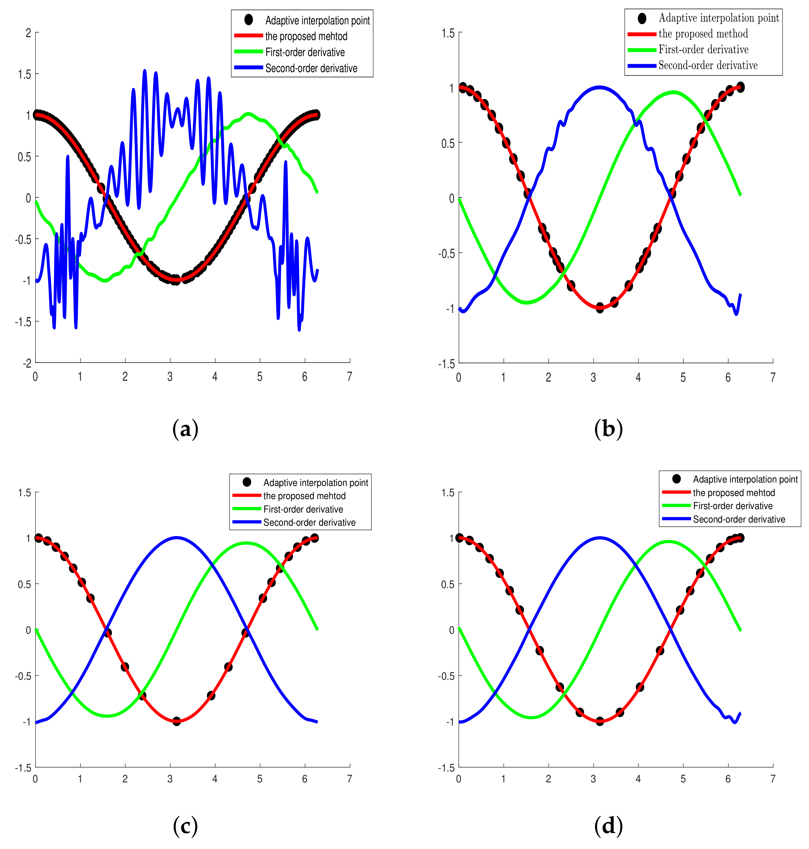
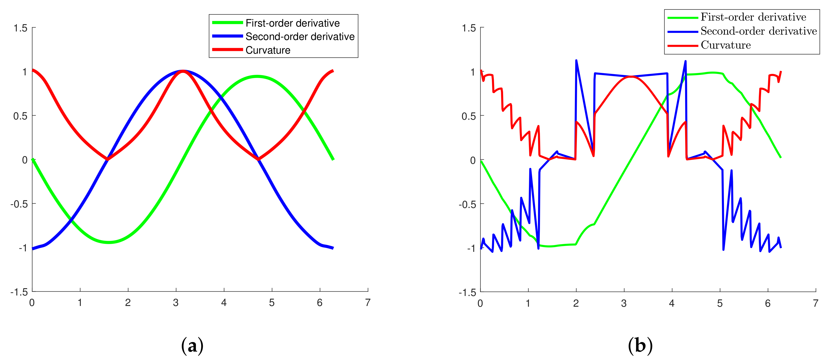
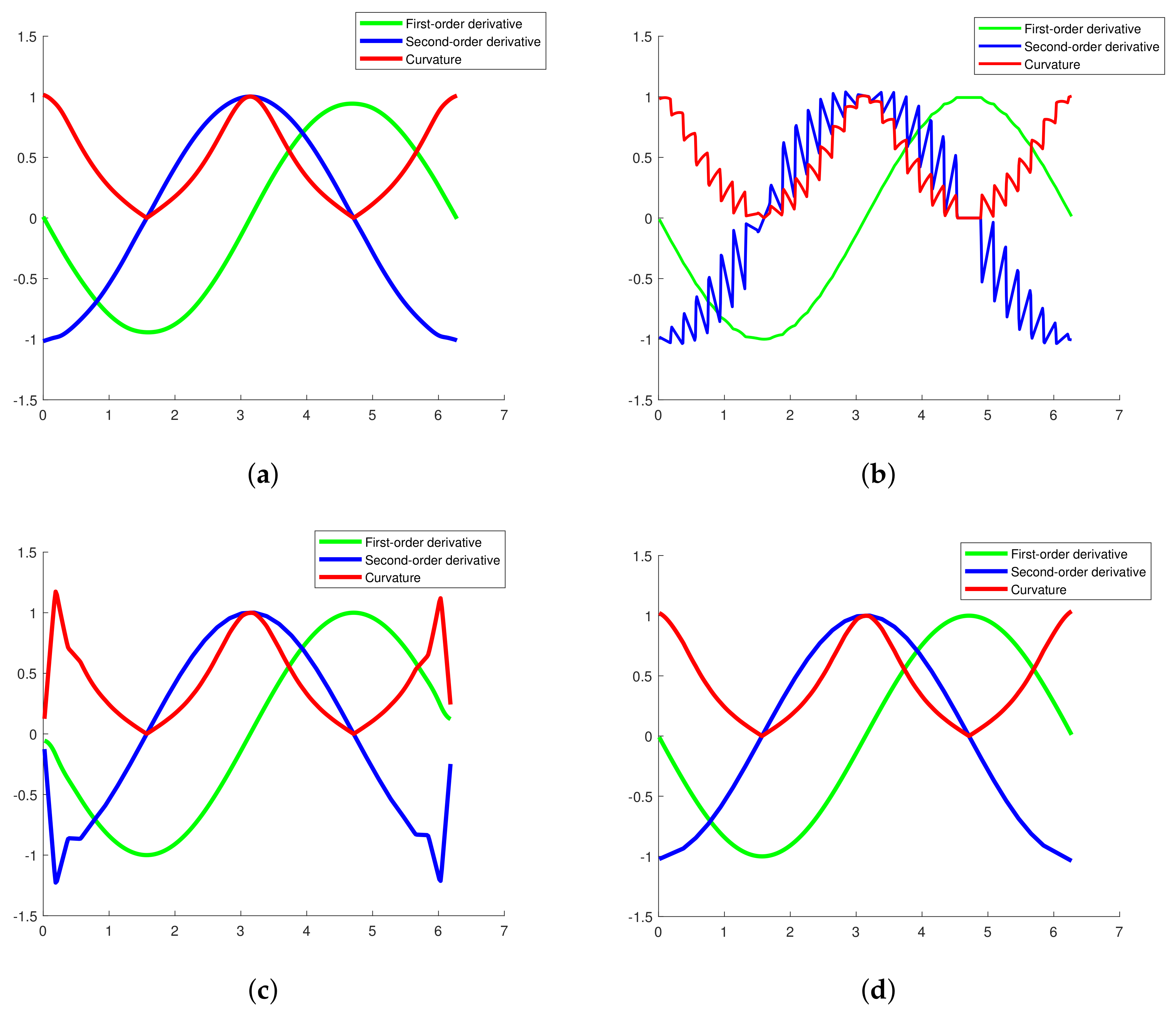
Compared with Shannon-Cosine interpolation wavelet method, the interval wavelet constructed in this paper reduces the boundary effect and avoids the phenomenon of infinite oscillation.

(2)

The wavelet multi-scale interpolation operator constructed in this paper is sensitive to the change of the gradient. According to this character, sparse feature interpolation points can be obtained adaptively.

(3)

Numerical Experiments 1 and 2 show that the proposed method is suitable for the reconstruction of infinitely derivable smooth and irregular functions. When the number of interpolation points is the same, the proposed method has smaller maximum error, absolute mean error, mean square error and running time. When achieving close accuracy, the other methods need to add more interpolation points, which increases the running time. The proposed method can reconstruct smooth curve with as few points as possible, and improve the efficiency of reconstruction.

(4)

The infinitely derivable smooth function reconstructed by the proposed method is smoother and satisfies $C^2$ and $G^2$ continuity.

References

1. Deng, S.W.; Jia, Y.; Yao, X.M.; Liu, Z.N. A method of reconstructing complex stratigraphic surfaces with multitype fault constraints. Appl. Geophys. 2017, 14, 195–204. [Google Scholar] [CrossRef]
2. Kong, D.; Tian, X.; Kong, D.; Zhang, X.; Yuan, L. An Improved Method for NURBS Free-form Surface Based on Discrete Stationary Wavelet Transform. IEEE Access 2020, 8, 67015–67023. [Google Scholar] [CrossRef]
3. Fucile, P.; Papallo, I.; Improta, G.; De Santis, R.; Gloria, A.; Onofrio, I.; D’Antò, V.; Maietta, S.; Russo, T. Reverse Engineering and Additive Manufacturing towards the design of 3D advanced scaffolds for hard tissue regeneration. In Proceedings of the 2019 II Workshop on Metrology for Industry 4.0 and IoT (MetroInd4.0&IoT), Naples, Italy, 4–6 June 2019; pp. 33–37. [Google Scholar]
4. Ghaffar, A.; Iqbal, M.; Bari, M.; Muhammad Hussain, S.; Manzoor, R.; Sooppy Nisar, K.; Baleanu, D. Construction and Application of Nine-Tic B-Spline Tensor Product SS. Mathematics 2019, 7, 675. [Google Scholar] [CrossRef] [Green Version]
5. Aràndiga, F.; Donat, R.; Romani, L.; Rossini, M. On the reconstruction of discontinuous functions using multiquadric RBF–WENO local interpolation techniques. Math. Comput. Simul. 2020, 176, 4–24. [Google Scholar] [CrossRef]
6. Bhuiyan, S.M.A.; Attoh-Okine, N.O.; Barner, K.E.; Ayenu-Prah, A.Y.; Adhami, R.R. Bidimensional Empirical Mode Decomposition Using Various Interpolation Techniques. Adv. Adapt. Data Anal. 2009, 1, 309–338. [Google Scholar] [CrossRef]
7. Elhoseny, M.; Tharwat, A.; Hassanien, A.E. Bezier curve based path planning in a dynamic field using modified genetic algorithm. J. Comput. Sci. 2018, 25, 339–350. [Google Scholar] [CrossRef]
8. Penner, A. ODF Using a 5-Point B-Spline. In Fitting Splines to a Parametric Function; Springer: Berlin/Heidelberg, Germany, 2019; pp. 37–42. [Google Scholar]
9. Gavriil, K.; Schiftner, A.; Pottmann, H. Optimizing B-spline surfaces for developability and paneling architectural freeform surfaces. Comput. Aided Des. 2019, 111, 29–43. [Google Scholar] [CrossRef] [Green Version]
10. Gao, X.; Zhang, S.; Qiu, L.; Liu, X.; Wang, Z.; Wang, Y. Double B-Spline Curve-Fitting and Synchronization-Integrated Feedrate Scheduling Method for Five-Axis Linear-Segment Toolpath. Appl. Sci. 2020, 10, 3158. [Google Scholar] [CrossRef]
11. Otoguro, Y.; Takizawa, K.; Tezduyar, T.E. A general-purpose NURBS mesh generation method for complex geometries. In Frontiers in Computational Fluid-Structure Interaction and Flow Simulation; Springer: Berlin/Heidelberg, Germany, 2018; pp. 399–434. [Google Scholar]
12. Zhao, Z.; Zhang, Y.; He, L.; Chang, X.; Zhang, L. A large-scale parallel hybrid grid generation technique for realistic complex geometry. Int. J. Numer. Methods Fluids 2020, 92, 1235–1255. [Google Scholar] [CrossRef]
13. Zhang, Q.; Zhao, Y.; Levesley, J. Adaptive radial basis function interpolation using an error indicator. Numer. Algorithms 2017, 76, 441–471. [Google Scholar] [CrossRef] [Green Version]
14. Xu, S.Z.; Yu, H.L. The Interpolation-Iteration Method for Potential Field Continuation from Undulating Surface to Plane. Chin. J. Geophys. 2007, 50, 1566–1570. [Google Scholar] [CrossRef]
15. Feng, G. Research of Multiresolution Representation for Curves and Surfaces Based on Subdivision. Master’s Thesis, Northwestern Polytechnical University, Xi’an, China, 2015. [Google Scholar]
16. Harti, A. Discrete multi-resolution analysis and generalized wavelets. Appl. Numer. Math. 1993, 12, 153–192. [Google Scholar] [CrossRef]
17. Ho, D.K.; Plodpradista, P. On the use of multiresolution analysis for subsurface object detection using deep ground penetrating radar. In Detection and Sensing of Mines, Explosive Objects, and Obscured Targets XXIV; International Society for Optics and Photonics: Bellingham, WA, USA, 2019; Volume 11012, p. 1101209. [Google Scholar]
18. Matei, B.; Meignen, S. Nonlinear cell-average multiscale signal representations: Application to signal denoising. Signal Process. 2012, 92, 2738–2746. [Google Scholar] [CrossRef]
19. Bayer, F.M.; Kozakevicius, A.J.; Cintra, R.J. An iterative wavelet threshold for signal denoising. Signal Process. 2019, 162, 10–20. [Google Scholar] [CrossRef]
20. Mei, S.; Gao, W. Shannon–Cosine wavelet spectral method for solving fractional Fokker–Planck equations. Int. J. Wavel. Multiresolut. Inf. Process. 2018, 16, 1850021. [Google Scholar] [CrossRef] [Green Version]
21. Mei, S.; Liu, X.; Mei, S. Cell-filtering Based Multi-scale Shannon-Cosine Wavelet Denoising Method for Locust Slice Images. Int. J. Wavel. Multiresolut. Inf. Process. 2019, 17, 1950035. [Google Scholar] [CrossRef]
22. Xing, R.; Li, Y.; Wang, Q.; Wu, Y.; Mei, S.L. Point-Symmetric Extension-Based Interval Shannon-Cosine Spectral Method for Fractional PDEs. Discret. Dyn. Nat. Soc. 2020, 2020, 4565036. [Google Scholar] [CrossRef]
23. Lee, W.S.; Kassim, A.A. Signal and image approximation using interval wavelet transform. IEEE Trans. Image Process. 2006, 16, 46–56. [Google Scholar] [CrossRef] [Green Version]
24. Mei, S.L.; Zhu, D.H. Interval shannon wavelet collocation method for fractional fokker-planck equation. Adv. Math. Phys. 2013, 2013, 821820. [Google Scholar] [CrossRef] [Green Version]
25. Hou, Z.; Wang, C.; Yang, A. Study on symmetric extension methods in Mallat algorithm of finite length signal. In Proceedings of the 5th International Conference on Visual Information Engineering, Xi’an, China, 29 July–1 August 2009. [Google Scholar]
26. Huang, G.; Nammour, R.; Symes, W.W.; Dolliazal, M. Waveform inversion via source extension. In SEG Technical Program Expanded Abstracts 2019; Society of Exploration Geophysicists: Tulsa, OK, USA, 2019; pp. 4761–4766. [Google Scholar]
27. Ma, S.; Pan, F. Symmetric Extension of Steering Vectors and Beamforming. Prog. Electromagn. Res. 2018, 76, 19–29. [Google Scholar] [CrossRef] [Green Version]
28. Han, B.; Michelle, M. Construction of wavelets and framelets on a bounded interval. Anal. Appl. 2018, 16, 807–849. [Google Scholar] [CrossRef]
29. Reidl, F.; Wahlström, M. Parameterized Algorithms for Zero Extension and Metric Labelling Problems. arXiv 2018, arXiv:1802.06026. [Google Scholar]
30. Zhengkun, L.; Ze, Z. The improved algorithm of the EMD endpoint effect based on the mirror continuation. In Proceedings of the 2016 Eighth International Conference on Measuring Technology and Mechatronics Automation (ICMTMA), Macau, China, 11–12 March 2016; pp. 792–795. [Google Scholar]
31. Williams, J.R.; Amaratunga, K. A Discrete Wavelet Transform without edge effects using wavelet extrapolation. J. Fourier Anal. Appl. 1997, 3, 435–449. [Google Scholar] [CrossRef] [Green Version]
32. Xiang, J.; Chen, X.; He, Y.; He, Z. The construction of plane elastomechanics and Mindlin plate elements of B-spline wavelet on the interval. Finite Elem. Anal. Des. 2006, 42, 1269–1280. [Google Scholar] [CrossRef]
33. Xiang, J.; Chen, X.; Li, B.; He, Z.; He, Y. The construction of two-dimensional plane elasticity element using B-spline wavelet on the interval. In Proceedings of the 6th International Progress on Wavelet Analysis and Active Media Technology; World Scientific Publishing: Singapore, 2005. [Google Scholar]
34. Donovan, G.C.; Geronimo, J.S.; Hardin, D.P. Orthogonal polynomials and the construction of piecewise polynomial smooth wavelets. SIAM J. Math. Anal. 1999, 30, 1029–1056. [Google Scholar] [CrossRef] [Green Version]
35. Kilgore, T.; Prestin, J. Polynomial Wavelets on the Interval. Constr. Approx. 1996, 12, 95–110. [Google Scholar] [CrossRef]
36. Fröhlich, J.; Uhlmann, M. Orthonormal polynomial wavelets on the interval and applications to the analysis of turbulent fields. SIAM J. Appl. Math. 2003, 63, 1789–1830. [Google Scholar] [CrossRef]
37. Xiang, J.; Matsumoto, T.; Wang, Y.; Jiang, Z. A Hybrid of Interval Wavelets and Wavelet Finite Element Model for Damage Detection in Structures. Comput. Model. Eng. Sci. 2011, 81, 269–294. [Google Scholar]
38. Boshernitzan, M.D.; Carroll, C. An extension of Lagrange’s theorem to interval exchange transformations over quadratic fields. J. d’Anal. Math. 1997, 72, 21–44. [Google Scholar] [CrossRef]
39. Phelan, C.E.; Marazzina, D.; Fusai, G.; Germano, G. Hilbert transform, spectral filters and option pricing. Ann. Oper. Res. 2019, 282, 273–298. [Google Scholar] [CrossRef] [Green Version]
40. Zhang, Y.; Wei, Y.; Mei, S.; Zhu, M. Application of multi-scale interval interpolation wavelet in beef image of marbling segmentation. Trans. Chin. Soc. Agric. Eng. 2016, 32, 296–304. [Google Scholar]
41. Wei, Y.; Zhang, Y.; Mei, S.; Wei, S. Image dehazing method based on dark channel prior and interval interpolation wavelet transform. Trans. Chin. Soc. Agric. Eng. 2017, 33, 281–287. [Google Scholar]
42. Kumar, A.; Pooja, R.; Singh, G.K. Design and performance of closed form method for cosine modulated filter bank using different windows functions. Int. J. Speech Technol. 2014, 17, 427–441. [Google Scholar] [CrossRef]
43. Comert, Z.; Boopathi, A.M.; Velappan, S.; Yang, Z.; Kocamaz, A.F. The influences of different window functions and lengths on image-based time-frequency features of fetal heart rate signals. In Proceedings of the 2018 26th Signal Processing and Communications Applications Conference (SIU), Izmir, Turkey, 2–5 May 2018. [Google Scholar]
44. Cheng, B.; Jin, L.; Li, G. Infrared and visual image fusion using LNSST and an adaptive dual-channel PCNN with triple-linking strength. Neurocomputing 2018, 310, 135–147. [Google Scholar] [CrossRef]
45. Agarwal, P.; Singh, S.P.; Pandey, V.K. Mathematical analysis of blackman window function in fractional Fourier transform domain. In Proceedings of the International Conference on Medical Imaging, Greater Noida, India, 7–8 November 2014. [Google Scholar]
46. Dimofte, C.; Mihut, L.; Baltog, I. Gauss window for singular system analysis in granulometry. In ROMOPTO’94: Fourth Conference in Optics; International Society for Optics and Photonics: Bellingham, WA, USA, 1995. [Google Scholar]
47. Pan, S.; Han, Y.; Wei, S.; Wei, Y.; Xia, L.; Xie, L.; Kong, X.; Yu, W. A model based on Gauss Distribution for predicting window behavior in building. Build. Environ. 2019, 149, 210–219. [Google Scholar] [CrossRef]
48. Hoffman, D.; Wei, G.; Zhang, D.; Kouri, D. Shannon–Gabor wavelet distributed approximating functional. Chem. Phys. Lett. 1998, 287, 119–124. [Google Scholar] [CrossRef]
49. Shuli, M. Study on Wavelet Stochastic Finite Element Method. Ph.D. Thesis, China Agriculture University, Beijing, China, 2002. [Google Scholar]
50. Chakrabarti, D.; Sahutoglu, S. The restriction operator on Bergman spaces. J. Geom. Anal. 2020, 30, 2157–2188. [Google Scholar] [CrossRef] [Green Version]
51. Liu, P.P.; Wei, H.Z.; Chen, C.R.; Li, S.J. Continuity of Solutions for Parametric Set Optimization Problems via Scalarization Methods. J. Oper. Res. Soc. China 2018, 1–19. [Google Scholar] [CrossRef]
52. Hu, G.; Bo, C.; Qin, X. Continuity conditions for Q-Bézier curves of degree n. J. Inequal. Appl. 2017, 2017, 115. [Google Scholar] [CrossRef] [Green Version]
53. Daubechies, I. Where Do Wavelets Come From? A Personal Point of View. Proc. IEEE 1996, 84, 510–513. [Google Scholar] [CrossRef] [Green Version]
Figure 1. Comparison between Shannon wavelet scale function sinc(x) and Shannon-Cosine wavelet scale function Sc(X): (a) Shannon wavelet scale function; and (b) Shannon-Cosine wavelet scale function Sc(X), m = 3.
Mathematics 09 00001 g001aMathematics 09 00001 g001b
Figure 2. Extension diagram of Hermite method: (a) the first-order derivative is positive; (b) the first-order derivative is zero; and (c) the first derivative is negative.
Mathematics 09 00001 g002
Figure 3. Schematic diagram of segmented interval wavelet.
Mathematics 09 00001 g003
Figure 4. Schematic diagram of wavelet reconstruction curve: (a) Shannon-Gabor wavelet; and (b) Shannon-Cosine interpolation wavelet.
Mathematics 09 00001 g004
Figure 5. Schematic diagram of interval wavelet reconstruction curve: (a) interval Shannon–Gabor wavelet; and (b) interval Shannon-Cosine wavelet.
Mathematics 09 00001 g005
Figure 6. Selection of extension interval: (a) extension interval is 1; (b) extension interval is 2; (c) extension interval is 3; and (d) extension interval is 4.
Mathematics 09 00001 g006
Figure 7. Comparison of reconstruction error between the proposed method and other methods: (a) the number of interpolation points is 21; and (b) the number of interpolation points is 34.
Mathematics 09 00001 g007
Figure 8. Comparison of reconstruction curve properties between the proposed method and other methods, when the number of interpolation points is 21: (a) the proposed method; (b) akima method; (c) Bezier method; and (d) cubic spline method.
Mathematics 09 00001 g008aMathematics 09 00001 g008b
Figure 9. Comparison of reconstruction curve properties between the proposed method and other methods, when the number of interpolation points is 34: (a) the proposed method; (b) akima method; (c) Bezier method; and (d) cubic spline method.
Mathematics 09 00001 g009
Figure 10. Comparison of reconstruction error between the proposed method and other methods: (a) the number of interpolation points is 9; and (b) the number of interpolation points is 17.
Mathematics 09 00001 g010