Modeling Soil Water Redistribution under Gravity Irrigation with the Richards Equation

Abstract

Soil water movement is important in fields such as soil mechanics, irrigation, drainage, hydrology, and agriculture. The Richards equation describes the flow of water in an unsaturated porous medium, and analytical solutions exist only for simplified cases. However, numerous practical situations require a numerical solution (1D, 2D, or 3D) depending on the complexity of the studied problem. In this paper, numerical solution of the equation describing water infiltration into soil using the finite difference method is studied. The finite difference solution is made via iterative schemes of local balance, including explicit, implicit, and intermediate methods; as a special case, the Laasonen method is shown. The found solution is applied to water transfer problems during and after gravity irrigation to observe phenomena of infiltration, evaporation, transpiration, and percolation.

1. Introduction

Surface gravity irrigation consists of the supply of water at the head of a channel or inclined channel built on a plot, such as a border or a furrow, to take advantage of the gravitational field and provide the necessary amount of water for the development of cultivated plants [1,2].

In surface gravity irrigation, there are three phases—the advanced phase, the storage phase, and the recession phase—which together are studied using a variety of models to understand the phenomenon [3], ranging from empirical to physical-based models that use the Barré de Saint-Venant [4] and Richards equations [5] to model the surface movement and underground movement, respectively [2].

The differential equation that describes the water transfer in soils [5] is difficult to integrate in an analytical way for most initial and boundary conditions of practical interest, due to its highly nonlinear nature [2,3,4,5,6]. This situation leads to the use of numerical methods for their integration and application in simulations of the moisture profile evolution and of the infiltrated depth during gravity irrigation [2,7,8,9], and also in simulations of water redistribution after irrigation due to the gravitational field, water evaporation through the soil surface, and crop transpiration [7,8,9].

The general equation of water transfer in soil,

$$\frac{\partial \mathsf{\theta }}{\partial \mathrm{t}}=\nabla \cdot \left[\mathrm{K}\left(\mathsf{\psi }\right)\nabla \mathsf{\psi }\right]-\frac{\mathrm{d}\mathrm{K}}{\mathrm{d}\mathsf{\psi }}\frac{\partial \mathsf{\psi }}{\partial \mathrm{z}}-\mathsf{\Upsilon },$$

(1)

results from the combination of the continuity equation which results from the principle of conservation of mass,

$$\frac{\partial \mathsf{\theta }}{\partial \mathrm{t}}+\nabla \cdot \mathbf{q}+\mathsf{\Upsilon }=0,$$

(2)

and from Darcy’s Law [10], argued experimentally, which represents the dynamic equation resulting from the principle of the amount of momentum:

$$\mathbf{q}=-\mathrm{K}\left(\mathsf{\psi }\right)\nabla \mathrm{H},\mathrm{H}=\mathsf{\psi }-\mathrm{z}$$

(3)

where $\mathsf{\theta }$ is the volumetric water content, also known as the moisture content; q = (q_x, q_y, q_z) is the flow of water per unit area of soil or Darcy flow, with its components in the directions of space (x,y,z); t is the time; $\mathsf{\Upsilon }$ is a term of source or sink as the volume of extracted water by plants per unit volume of soil and unit of time; H is the hydraulic potential or hydraulic load, being equal to the sum of pressure potential ($\mathsf{\psi }$), which is negative in the unsaturated area of soil and positive in the saturated area, and the gravitational potential assimilated to the vertical coordinate positively oriented downward (z); and K is the hydraulic conductivity of the partially saturated soil and depends on pressure or moisture content. The relationships θ(ψ) and K(ψ) are called soil hydrodynamic characteristics.

The differential equation contains two apparently dependent variables, namely, the moisture content and water pressure, but these are related through the retention curve. With the introduction in the equation of the specific capacity, defined as the slope of the curve retention C($\mathsf{\psi }$) = $\mathrm{d}\mathsf{\theta }$/$\mathrm{d}\mathsf{\psi }$, that is,

$$\frac{\partial \mathsf{\theta }}{\partial \mathrm{t}}=\mathrm{C}\left(\mathsf{\psi }\right)\frac{\partial \mathsf{\psi }}{\partial \mathrm{t}},$$

(4)

the pressure only appears to be a dependent variable; this is known as the Richards equation [5].

As for the analytical representation of the hydrodynamic characteristics, according to [11], the combination of the hydrodynamic characteristics of Fujita [12] and Parlange [13] is used for theoretical studies, such as the construction of exact analytical solutions; in experimental studies, a combination of the retention curve proposed by van Genuchten [14] is used, considering the restriction of Burdine [15], with the curve of hydraulic conductivity proposed by Brooks and Corey [16], due to the fact that they satisfy the integral properties of infiltration and easy identification of its parameters.

In this study, we focus on solving the Richards vertical one-dimensional differential equation:

$$\mathrm{C}\left(\mathsf{\psi }\right)\frac{\partial \mathsf{\psi }}{\partial \mathrm{t}}=\frac{\partial }{\partial \mathrm{z}}\left[\mathrm{K}\left(\mathsf{\psi }\right)\left(\frac{\partial \mathsf{\psi }}{\partial \mathrm{z}}-1\right)\right]-\mathsf{\Upsilon }$$

(5)

which is a combination of the continuity equation,

$$\frac{\partial \mathsf{\theta }}{\partial \mathrm{t}}+\frac{\partial {\mathrm{q}}_{\mathrm{z}}}{\partial \mathrm{z}}=-\mathsf{\Upsilon },$$

(6)

and Darcy’s Law,

$${\mathrm{q}}_{\mathrm{z}}=\mathrm{K}\left(\mathsf{\psi }\right)-\mathrm{K}\left(\mathsf{\psi }\right)\frac{\partial \mathsf{\psi }}{\partial \mathrm{z}}.$$

(7)

2. Materials and Methods

2.1. Solution in Finite Difference by Local Balance of Mass

To build the numerical solution, a scheme proposed by Zataráin et al. [17] was used. According to the algorithm, the soil profile is divided into layers that may be non-constant, as shown in Figure 1. The interpolation parameters are introduced and defined by

$${\mathsf{\gamma }}_{\mathrm{z}}=\frac{{\mathrm{z}}_{\mathrm{i}+{\mathsf{\gamma }}_{\mathrm{z}}}-{\mathrm{z}}_{\mathrm{i}}}{{\mathrm{z}}_{\mathrm{i}+1}-{\mathrm{z}}_{\mathrm{i}}};\mathsf{\omega }=\frac{{\mathrm{t}}_{\mathrm{k}+\mathsf{\omega }}-{\mathrm{t}}_{\mathrm{k}}}{{\mathrm{t}}_{\mathrm{k}+1}-{\mathrm{t}}_{\mathrm{k}}}$$

(8)

where 0$\le$γ_z$\le$1 and $0\le \mathsf{\omega }\le 1$; $\mathrm{i}=1,2,\dots$ and $\mathrm{k}=1,2,\dots$ are the indices for space and time, respectively. The discretization of the equations assumes that the weighting factors are independent of space and time.

The pressure ψ in an intermediate node i + γ_z for all k is estimated via

$${\mathsf{\psi }}_{\mathrm{i}+{\mathsf{\gamma }}_{\mathrm{z}}}^{\mathrm{k}}=\left(1-{\mathsf{\gamma }}_{\mathrm{z}}\right){\mathsf{\psi }}_{\mathrm{i}}^{\mathrm{k}}+{\mathsf{\gamma }}_{\mathrm{z}}{\mathsf{\psi }}_{\mathrm{i}+1}^{\mathrm{k}}.$$

(9)

The pressure ${\mathsf{\psi }}_{\mathrm{i}-1+{\mathsf{\gamma }}_{\mathrm{z}}}^{\mathrm{k}}$ is deduced by replacing i with i−1 in Equation (9), and the pressure at the intermediate time k + ω for all i is estimated as

$${\mathsf{\psi }}_{\mathrm{i}}^{\mathrm{k}+\mathsf{\omega }}=\left(1-\mathsf{\omega }\right){\mathsf{\psi }}_{\mathrm{i}}^{\mathrm{k}}+\mathsf{\omega }{\mathsf{\psi }}_{\mathrm{i}}^{\mathrm{k}+1}.$$

(10)

The time derivative of Equation (6) for the ith node is calculated as follows:

$${\frac{\partial \mathsf{\theta }}{\partial \mathrm{t}}|}_{\mathrm{i}}^{\mathrm{k}+\mathsf{\omega }}={\mathrm{C}\left(\mathsf{\psi }\right)\frac{\partial \mathsf{\psi }}{\partial \mathrm{t}}|}_{\mathrm{i}}^{\mathrm{k}+\mathsf{\omega }}=\frac{{\mathrm{C}}_{\mathrm{i}}^{\mathrm{k}+\mathsf{\omega }}}{\Delta {\mathrm{t}}_{\mathrm{k}}}\left({\mathsf{\psi }}_{\mathrm{i}}^{\mathrm{k}+1}-{\mathsf{\psi }}_{\mathrm{i}}^{\mathrm{k}}\right);\Delta {\mathrm{t}}_{\mathrm{k}}={\mathrm{t}}_{\mathrm{k}+1}-{\mathrm{t}}_{\mathrm{k}}$$

(11)

where ${\mathrm{C}}_{\mathrm{i}}^{\mathrm{k}+\mathsf{\omega }}=\mathrm{C}\left({\mathsf{\psi }}_{\mathrm{i}}^{\mathrm{k}+\mathsf{\omega }}\right)$.

The discretization of the spatial derivative in Equation (6) is

$${\frac{\partial {\mathrm{q}}_{\mathrm{z}}}{\partial \mathrm{z}}|}_{\mathrm{i}}^{\mathrm{k}+\mathsf{\omega }}=\frac{{{\mathrm{q}}_{\mathrm{z}}|}_{\mathrm{i}+{\mathsf{\gamma }}_{\mathrm{z}}}^{\mathrm{k}+\mathsf{\omega }}-{{\mathrm{q}}_{\mathrm{z}}|}_{\mathrm{i}-1+{\mathsf{\gamma }}_{\mathrm{z}}}^{\mathrm{k}+\mathsf{\omega }}}{\Delta {\mathrm{z}}_{\mathrm{i}}};\Delta {\mathrm{z}}_{\mathrm{i}}=\left(1-{\mathsf{\gamma }}_{\mathrm{z}}\right)\left({\mathrm{z}}_{\mathrm{i}}-{\mathrm{z}}_{\mathrm{i}-1}\right)+{\mathsf{\gamma }}_{\mathrm{z}}\left({\mathrm{z}}_{\mathrm{i}+1}-{\mathrm{z}}_{\mathrm{i}}\right).$$

(12)

According to Equation (7),

$${{\mathrm{q}}_{\mathrm{z}}|}_{\mathrm{i}+{\mathsf{\gamma }}_{\mathrm{z}}}^{\mathrm{k}+\mathsf{\omega }}={\mathrm{K}}_{\mathrm{i}+{\mathsf{\gamma }}_{\mathrm{z}}}^{\mathrm{k}+\mathsf{\omega }}-{\mathrm{K}}_{\mathrm{i}+{\mathsf{\gamma }}_{\mathrm{z}}}^{\mathrm{k}+\mathsf{\omega }}\frac{{\mathsf{\psi }}_{\mathrm{i}+1}^{\mathrm{k}+\mathsf{\omega }}-{\mathsf{\psi }}_{\mathrm{i}}^{\mathrm{k}+\mathsf{\omega }}}{{\mathrm{z}}_{\mathrm{i}+1}-{\mathrm{z}}_{\mathrm{i}}},$$

(13)

where ${\mathrm{K}}_{\mathrm{i}+{\mathsf{\gamma }}_{\mathrm{z}}}^{\mathrm{k}+\mathsf{\omega }}=\mathrm{K}\left({\mathsf{\psi }}_{\mathrm{i}+{\mathsf{\gamma }}_{\mathrm{z}}}^{\mathrm{k}+\mathsf{\omega }}\right)$. The flow ${{\mathrm{q}}_{\mathrm{z}}|}_{\mathrm{i}-1+{\mathsf{\gamma }}_{\mathrm{z}}}^{\mathrm{k}+\mathsf{\omega }}$ is deduced by replacing i with i−1 in Equation (13).

Thus, the divergence defined by Equation (12) is as follows:

$${\frac{\partial {\mathrm{q}}_{\mathrm{z}}}{\partial \mathrm{z}}|}_{\mathrm{i}}^{\mathrm{k}+\mathsf{\omega }}=\frac{{\mathrm{K}}_{\mathrm{i}+{\mathsf{\gamma }}_{\mathrm{z}}}^{\mathrm{k}+\mathsf{\omega }}}{\Delta {\mathrm{z}}_{\mathrm{i}}}-\frac{{\mathrm{K}}_{\mathrm{i}+{\mathsf{\gamma }}_{\mathrm{z}}}^{\mathrm{k}+\mathsf{\omega }}}{\Delta {\mathrm{z}}_{\mathrm{i}}\left({\mathrm{z}}_{\mathrm{i}+1}-{\mathrm{z}}_{\mathrm{i}}\right)}\left({\mathsf{\psi }}_{\mathrm{i}+1}^{\mathrm{k}+\mathsf{\omega }}-{\mathsf{\psi }}_{\mathrm{i}}^{\mathrm{k}+\mathsf{\omega }}\right)-\frac{{\mathrm{K}}_{\mathrm{i}-1+{\mathsf{\gamma }}_{\mathrm{z}}}^{\mathrm{k}+\mathsf{\omega }}}{\Delta {\mathrm{z}}_{\mathrm{i}}}+\frac{{\mathrm{K}}_{\mathrm{i}-1+{\mathsf{\gamma }}_{\mathrm{z}}}^{\mathrm{k}+\mathsf{\omega }}}{\Delta {\mathrm{z}}_{\mathrm{i}}\left({\mathrm{z}}_{\mathrm{i}}-{\mathrm{z}}_{\mathrm{i}-1}\right)}\left({\mathsf{\psi }}_{\mathrm{i}}^{\mathrm{k}+\mathsf{\omega }}-{\mathsf{\psi }}_{\mathrm{i}-1}^{\mathrm{k}+\mathsf{\omega }}\right).$$

(14)

The dependent variable involved in the hydraulic conductivity of Equation (13) is defined as

$${\mathsf{\psi }}_{\mathrm{i}+{\mathsf{\gamma }}_{\mathrm{z}}}^{\mathrm{k}+\mathsf{\omega }}=\left(1-\mathsf{\omega }\right){\mathsf{\psi }}_{\mathrm{i}+{\mathsf{\gamma }}_{\mathrm{z}}}^{\mathrm{k}}+\mathsf{\omega }{\mathsf{\psi }}_{\mathrm{i}+{\mathsf{\gamma }}_{\mathrm{z}}}^{\mathrm{k}+1}=\left(1-\mathsf{\omega }\right)\left[\left(1-{\mathsf{\gamma }}_{\mathrm{z}}\right){\mathsf{\psi }}_{\mathrm{i}}^{\mathrm{k}}+{\mathsf{\gamma }}_{\mathrm{z}}{\mathsf{\psi }}_{\mathrm{i}+1}^{\mathrm{k}}\right]+\mathsf{\omega }\left[\left(1-{\mathsf{\gamma }}_{\mathrm{z}}\right){\mathsf{\psi }}_{\mathrm{i}}^{\mathrm{k}+1}+{\mathsf{\gamma }}_{\mathrm{z}}{\mathsf{\psi }}_{\mathrm{i}+1}^{\mathrm{k}+1}\right].$$

(15)

The pressure ${\mathsf{\psi }}_{\mathrm{i}-1+{\mathsf{\gamma }}_{\mathrm{z}}}^{\mathrm{k}+\mathsf{\omega }}$ is deduced replacing i with i−1 in Equation (15). Substituting Equation (10) into Equation (14) and this, in turn, into Equation (6) together with Equation (11) leads to the following system of algebraic equations:

$${\mathrm{A}}_{\mathrm{i}}{\mathsf{\psi }}_{\mathrm{i}-1}^{\mathrm{k}+1}+{\mathrm{B}}_{\mathrm{i}}{\mathsf{\psi }}_{\mathrm{i}}^{\mathrm{k}+1}+{\mathrm{D}}_{\mathrm{i}}{\mathsf{\psi }}_{\mathrm{i}+1}^{\mathrm{k}+1}={\mathrm{E}}_{\mathrm{i}};\mathrm{i}=2,3,\dots ,\mathrm{n}-1$$

(16)

where

$${\mathrm{A}}_{\mathrm{i}}=-\mathsf{\omega }\frac{{\mathrm{K}}_{\mathrm{i}-1+{\mathsf{\gamma }}_{\mathrm{z}}}^{\mathrm{k}+\mathsf{\omega }}}{\Delta {\mathrm{z}}_{\mathrm{i}}\left({\mathrm{z}}_{\mathrm{i}}-{\mathrm{z}}_{\mathrm{i}-1}\right)},$$

(17)

$${\mathrm{D}}_{\mathrm{i}}=-\mathsf{\omega }\frac{{\mathrm{K}}_{\mathrm{i}+{\mathsf{\gamma }}_{\mathrm{z}}}^{\mathrm{k}+\mathsf{\omega }}}{\Delta {\mathrm{z}}_{\mathrm{i}}\left({\mathrm{z}}_{\mathrm{i}+1}-{\mathrm{z}}_{\mathrm{i}}\right)},$$

(18)

$${\mathrm{B}}_{\mathrm{i}}=\frac{{\mathrm{C}}_{\mathrm{i}}^{\mathrm{k}+\mathsf{\omega }}}{\Delta {\mathrm{t}}_{\mathrm{k}}}-{\mathrm{A}}_{\mathrm{i}}-{\mathrm{D}}_{\mathrm{i}},$$

(19)

$$\begin{array}{cc}{\mathrm{E}}_{\mathrm{i}}=& \frac{\left(1-\mathsf{\omega }\right){\mathrm{K}}_{\mathrm{i}-1+{\mathsf{\gamma }}_{\mathrm{z}}}^{\mathrm{k}+\mathsf{\omega }}}{\Delta {\mathrm{z}}_{\mathrm{i}}\left({\mathrm{z}}_{\mathrm{i}}-{\mathrm{z}}_{\mathrm{i}-1}\right)}{\mathsf{\psi }}_{\mathrm{i}-1}^{\mathrm{k}}+\left\{\frac{{\mathrm{C}}_{\mathrm{i}}^{\mathrm{k}+\mathsf{\omega }}}{\Delta {\mathrm{t}}_{\mathrm{k}}}-\frac{1-\mathsf{\omega }}{\Delta {\mathrm{z}}_{\mathrm{i}}}\left[\frac{{\mathrm{K}}_{\mathrm{i}+{\mathsf{\gamma }}_{\mathrm{z}}}^{\mathrm{k}+\mathsf{\omega }}}{\left({\mathrm{z}}_{\mathrm{i}+1}-{\mathrm{z}}_{\mathrm{i}}\right)}+\frac{{\mathrm{K}}_{\mathrm{i}-1+{\mathsf{\gamma }}_{\mathrm{z}}}^{\mathrm{k}+\mathsf{\omega }}}{\left({\mathrm{z}}_{\mathrm{i}}-{\mathrm{z}}_{\mathrm{i}-1}\right)}\right]\right\}{\mathsf{\psi }}_{\mathrm{i}}^{\mathrm{k}}\hfill \\ & +\frac{\left(1-\mathsf{\omega }\right){\mathrm{K}}_{\mathrm{i}+{\mathsf{\gamma }}_{\mathrm{z}}}^{\mathrm{k}+\mathsf{\omega }}}{\Delta {\mathrm{z}}_{\mathrm{i}}\left({\mathrm{z}}_{\mathrm{i}+1}-{\mathrm{z}}_{\mathrm{i}}\right)}{\mathsf{\psi }}_{\mathrm{i}+1}^{\mathrm{k}}+\frac{{\mathrm{K}}_{\mathrm{i}-1+{\mathsf{\gamma }}_{\mathrm{z}}}^{\mathrm{k}+\mathsf{\omega }}}{\Delta {\mathrm{z}}_{\mathrm{i}}}-\frac{{\mathrm{K}}_{\mathrm{i}+{\mathsf{\gamma }}_{\mathrm{z}}}^{\mathrm{k}+\mathsf{\omega }}}{\Delta {\mathrm{z}}_{\mathrm{i}}}-{\mathsf{\Upsilon }}_{\mathrm{i}}^{\mathrm{k}+\mathsf{\omega }}\hfill \end{array}.$$

(20)

It is important to note that the system is not linear since the coefficients (17)–(20) depend on the solution itself. Therefore, the resolution for each time step is iterative. The first estimator can be obtained by the Laasonen scheme, which is the result of considering that the coefficients, specific capacity, and hydraulic conductivity are calculated in the previous time step while the hydraulic gradient is calculated at the current time. The method is partially implicit, and the resulting algorithm is no longer iterative in a time step. The coefficients of the system of equations defined by Equation (16) are defined by the following expressions deduced from Equations (17)–(20):

$${\mathrm{A}}_{\mathrm{i}}=-\frac{{\mathrm{K}}_{\mathrm{i}-1+{\mathsf{\gamma }}_{\mathrm{z}}}^{\mathrm{k}}}{\Delta {\mathrm{z}}_{\mathrm{i}}\left({\mathrm{z}}_{\mathrm{i}}-{\mathrm{z}}_{\mathrm{i}-1}\right)},$$

(21)

$${\mathrm{D}}_{\mathrm{i}}=-\frac{{\mathrm{K}}_{\mathrm{i}+{\mathsf{\gamma }}_{\mathrm{z}}}^{\mathrm{k}}}{\Delta {\mathrm{z}}_{\mathrm{i}}\left({\mathrm{z}}_{\mathrm{i}+1}-{\mathrm{z}}_{\mathrm{i}}\right)},$$

(22)

$${\mathrm{B}}_{\mathrm{i}}=\frac{{\mathrm{C}}_{\mathrm{i}}^{\mathrm{k}}}{\Delta {\mathrm{t}}_{\mathrm{k}}}-{\mathrm{A}}_{\mathrm{i}}-{\mathrm{D}}_{\mathrm{i}},$$

(23)

$${\mathrm{E}}_{\mathrm{i}}=\frac{{\mathrm{C}}_{\mathrm{i}}^{\mathrm{k}}}{\Delta {\mathrm{t}}_{\mathrm{k}}}{\mathsf{\psi }}_{\mathrm{i}}^{\mathrm{k}}+\frac{{\mathrm{K}}_{\mathrm{i}-1+{\mathsf{\gamma }}_{\mathrm{z}}}^{\mathrm{k}}}{\Delta {\mathrm{z}}_{\mathrm{i}}}-\frac{{\mathrm{K}}_{\mathrm{i}+{\mathsf{\gamma }}_{\mathrm{z}}}^{\mathrm{k}}}{\Delta {\mathrm{z}}_{\mathrm{i}}}-{\mathsf{\Upsilon }}_{\mathrm{i}}^{\mathrm{k}}.$$

(24)

The system (16) forms a tridiagonal matrix and can be solved efficiently by an algorithm of Gaussian elimination known as the Thomas algorithm or double scan. The solution of system (16) has the form

$${\mathsf{\psi }}_{\mathrm{i}}^{\mathrm{k}+1}={\mathrm{F}}_{\mathrm{i}}-{\mathrm{G}}_{\mathrm{i}}{\mathsf{\psi }}_{\mathrm{i}+1}^{\mathrm{k}+1};\mathrm{i}=1,\dots ,\mathrm{n}-1.$$

(25)

From Equation (25), ${\mathsf{\psi }}_{\mathrm{i}-1}^{\mathrm{k}+1}={\mathrm{F}}_{\mathrm{i}-1}-{\mathrm{G}}_{\mathrm{i}-1}{\mathsf{\psi }}_{\mathrm{i}}^{\mathrm{k}+1}$ can be deduced, which, substituted into Equation (16), leads to Equation (25) provided that

$${\mathrm{F}}_{\mathrm{i}}=\frac{{\mathrm{E}}_{\mathrm{i}}-{\mathrm{A}}_{\mathrm{i}}{\mathrm{F}}_{\mathrm{i}-1}}{{\mathrm{B}}_{\mathrm{i}}-{\mathrm{A}}_{\mathrm{i}}{\mathrm{G}}_{\mathrm{i}-1}};\mathrm{i}=2,\dots ,\mathrm{n}-1,$$

(26)

$${\mathrm{G}}_{\mathrm{i}}=\frac{{\mathrm{D}}_{\mathrm{i}}}{{\mathrm{B}}_{\mathrm{i}}-{\mathrm{A}}_{\mathrm{i}}{\mathrm{G}}_{\mathrm{i}-1}};\mathrm{i}=2,\dots ,\mathrm{n}-1.$$

(27)

Equations (26) and (27) require knowledge of F₁ and G₁, which are deduced from the boundary condition in z = 0; this is the forward scan, i = 2, 3, …, n−1. Subsequently, ${\mathsf{\psi }}_{\mathrm{n}}^{\mathrm{k}+1}$ is defined from the boundary condition in z = L, and ${\mathsf{\psi }}_{\mathrm{i}}^{\mathrm{k}+1}$ is calculated for i = n−1, n−2, …, 1; this is the backward scan. If the coefficients in system (16) depend on the pressure itself, they are updated and the algorithm reapplied until the next estimator of the solution t_k+1 is equal, given an error criterion, to the previous estimator. The convergence can be accelerated if second-order algorithms like Newton’s method are used to find the pressure in a given time step.

2.2. Boundary Conditions

The boundary conditions can be grouped into three types: Dirichlet (first type), Neumann (second type), and Robbins (third type). In gravity irrigation (basin irrigation, border irrigation, or furrow irrigation), the Dirichlet condition on the upper boundary (water depth over the soil surface) is one of the main components, and its characterization is fundamental for irrigation design [2,6,7,8,9]. In this condition, the value of the dependent variable of the differential equation for all time on the soil surface (pressure) is known. It is introduced into the numerical solution by defining F₁ and G₁ from Equation (25). For the upper boundary, I = 1 is used in Equation (25), resulting in the following expression:

$${\mathsf{\psi }}_1^{\mathrm{k}+1}={\mathrm{F}}_1-{\mathrm{G}}_1{\mathsf{\psi }}_2^{\mathrm{k}+1}.$$

(28)

Due to the fact that ψ₁ is the water pressure on the soil surface and is independent of ψ₂, we have

$${\mathrm{F}}_1={\mathsf{\psi }}_1^{\mathrm{k}+1};{\mathrm{G}}_1=0.$$

(29)

For the lower boundary, the length of the column must be taken into consideration. In a semi-infinite column, pressure corresponds to the initial condition. In a finite column, pressure is introduced into the base position of the column by using i = n − 1 in Equation (25):

$${\mathsf{\psi }}_{\mathrm{n}-1}^{\mathrm{k}+1}={\mathrm{F}}_{\mathrm{n}-1}-{\mathrm{G}}_{\mathrm{n}-1}{\mathsf{\psi }}_{\mathrm{n}}^{\mathrm{k}+1}.$$

(30)

With this expression, the backward scan is performed.

2.3. The Analytical Solution of Infiltration

Equation (1) can be written with the moisture content as the dependent variable by introducing hydraulic diffusivity, defined as

$$\mathrm{D}\left(\mathsf{\theta }\right)=\mathrm{K}\left(\mathsf{\theta }\right)\frac{\mathrm{d}\mathsf{\psi }}{\mathrm{d}\mathsf{\theta }}.$$

(31)

The structure of the resulting equation corresponds to a nonlinear Fokker–Planck equation. The equation for one-dimensional vertical infiltration without a sink term is

$$\frac{\partial \mathsf{\theta }}{\partial \mathrm{t}}=\frac{\partial }{\partial \mathrm{z}}\left[\mathrm{D}\left(\mathsf{\theta }\right)\frac{\partial \mathsf{\theta }}{\partial \mathrm{z}}\right]-\frac{\mathrm{d}\mathrm{K}}{\mathrm{d}\mathsf{\theta }}\frac{\partial \mathsf{\theta }}{\partial \mathrm{z}}.$$

(32)

This equation defines the function θ = θ(z,t) for each type of initial and boundary conditions. Solutions can be built more or less simply considering that there is an implicit function z = z(θ,t), as in the case of infiltration in a semi-infinite column with a constant initial moisture content (θ₀) and constant humidity condition in the upper part of the column, generally equal to the moisture content at saturation (θ_s). From these considerations, the total differentials dθ = (∂θ/∂z)_t dz + (∂θ/∂t)_z dt and dz = (∂z/∂θ)_t dθ + (∂z/∂t)_θ are deduced, where the subscripts are the variables that remain constant in the differentiation. Substituting the first into the second, we have [(∂z/∂θ)_t(∂θ/∂t)_z + ((∂z/∂t)] dt = 0. The identity (∂z/∂θ)_t (∂θ/∂t)_z = −(∂z/∂t)_θ is then deduced, which allows us to write Equation (32) as follows:

$$\frac{\partial \mathrm{z}}{\partial \mathrm{t}}+\frac{\partial }{\partial \mathsf{\theta }}\left[\frac{\mathrm{D}\left(\mathsf{\theta }\right)}{\partial \mathrm{z}/\partial \mathsf{\theta }}\right]=\frac{\mathrm{d}\mathrm{K}}{\mathrm{d}\mathsf{\theta }}.$$

(33)

A first integration with the initial condition provides

$${\displaystyle \underset{{\mathsf{\theta }}_{\mathrm{o}}}{\overset{\mathsf{\theta }}{\int }}\frac{\partial \mathrm{z}}{\partial \mathrm{t}}\mathrm{d}\tilde{\mathsf{\theta }}}+\frac{\mathrm{D}\left(\mathsf{\theta }\right)}{\partial \mathrm{z}/\partial \mathsf{\theta }}=\mathrm{K}\left(\mathsf{\theta }\right)-{\mathrm{K}}_{\mathrm{o}}$$

(34)

where ${\mathrm{K}}_{\mathrm{o}}=\mathrm{K}\left({\mathsf{\theta }}_{\mathrm{o}}\right)$ is the initial hydraulic conductivity.

For the second integration, the relationship of the concentration of flows is introduced and defined as

$$\mathrm{F}\left(\mathsf{\theta },\mathrm{t}\right)={\displaystyle \underset{{\mathsf{\theta }}_{\mathrm{o}}}{\overset{\mathsf{\theta }}{\int }}\frac{\partial \mathrm{z}}{\partial \mathrm{t}}\mathrm{d}\tilde{\mathsf{\theta }}}/{\displaystyle \underset{{\mathsf{\theta }}_{\mathrm{o}}}{\overset{{\mathsf{\theta }}_{\mathrm{s}}}{\int }}\frac{\partial \mathrm{z}}{\partial \mathrm{t}}\mathrm{d}\tilde{\mathsf{\theta }}}=\frac{{\mathrm{q}}_{\mathrm{z}}\left(\mathsf{\theta },\mathrm{t}\right)-{\mathrm{K}}_{\mathrm{o}}}{{\mathrm{q}}_{\mathrm{s}}\left(\mathrm{t}\right)-{\mathrm{K}}_{\mathrm{o}}}$$

(35)

where ${\mathrm{q}}_{\mathrm{s}}\left(\mathrm{t}\right)={\mathrm{q}}_{\mathrm{z}}\left({\mathsf{\theta }}_{\mathrm{s}},\mathrm{t}\right)$ is the Darcy flux on the surface of the column or infiltration velocity.

From Equations (34) and (35), the moisture profile is deduced:

$$\mathrm{z}\left(\mathsf{\theta },\mathrm{t}\right)={\displaystyle \underset{\mathsf{\theta }}{\overset{{\mathsf{\theta }}_{\mathrm{s}}}{\int }}\frac{\mathrm{D}\left(\tilde{\mathsf{\theta }}\right)}{\mathrm{F}\left(\tilde{\mathsf{\theta }},\mathrm{t}\right)\left[{\mathrm{q}}_{\mathrm{s}}\left(\mathrm{t}\right)-{\mathrm{K}}_{\mathrm{o}}\right]-\left[\mathrm{K}\left(\tilde{\mathsf{\theta }}\right)-{\mathrm{K}}_{\mathrm{o}}\right]}\mathrm{d}\tilde{\mathsf{\theta }}},$$

(36)

in which the boundary condition $\mathrm{z}\left({\mathsf{\theta }}_{\mathrm{s}},\mathrm{t}\right)=0$ has been used.

The moisture profile integration provides water storage in the soil column:

$$\mathrm{I}\left(\mathrm{t}\right)-{\mathrm{K}}_{\mathrm{o}}\mathrm{t}={\displaystyle \underset{0}{\overset{\infty }{\int }}\left[\mathsf{\theta }\left(\mathrm{z},\mathrm{t}\right)-{\mathsf{\theta }}_{\mathrm{o}}\right]}\mathrm{d}\mathrm{z}={\displaystyle \underset{{\mathsf{\theta }}_{\mathrm{o}}}{\overset{{\mathsf{\theta }}_{\mathrm{s}}}{\int }}\frac{\left(\mathsf{\theta }-{\mathsf{\theta }}_{\mathrm{o}}\right)\mathrm{D}\left(\mathsf{\theta }\right)}{\mathrm{F}\left(\mathsf{\theta },\mathrm{t}\right)\left[{\mathrm{q}}_{\mathrm{s}}\left(\mathrm{t}\right)-{\mathrm{K}}_{\mathrm{o}}\right]-\left[\mathrm{K}\left(\mathsf{\theta }\right)-{\mathrm{K}}_{\mathrm{o}}\right]}\mathrm{d}\mathsf{\theta }},$$

(37)

where I(t) is the water depth accumulated over time, with q_s(t) = dI/dt.

Equations (36) and (37) can be integrated in an approximated manner using the hydrodynamic characteristics of Fujita [12] and Parlange [13]. Fujita diffusivity is provided by

$$\mathrm{D}\left(\mathsf{\theta }\right)=\frac{\left({\mathrm{K}}_{\mathrm{s}}-{\mathrm{K}}_0\right){\mathsf{\lambda }}_{\mathrm{c}}}{{\mathsf{\theta }}_{\mathrm{s}}-{\mathsf{\theta }}_0}\frac{1-\mathsf{\alpha }}{{\left(1-\mathsf{\alpha }{\mathsf{\theta }}_{\ast }\right)}^2};0<\mathsf{\alpha }<1$$

(38)

where $\mathsf{\alpha }$ is a shape parameter; K_s the hydraulic conductivity at saturation, and λ_c is the Bouwer scale [18] defined by

$${\mathsf{\lambda }}_{\mathrm{c}}=\frac{1}{{\mathrm{K}}_{\mathrm{s}}-{\mathrm{K}}_0}{\displaystyle \underset{{\mathsf{\theta }}_0}{\overset{{\mathsf{\theta }}_{\mathrm{s}}}{\int }}\mathrm{D}\left(\mathsf{\theta }\right)\mathrm{d}\mathsf{\theta }}$$

(39)

and the degree of saturation, ${\mathsf{\theta }}^{\ast }$, is defined by

$${\mathsf{\theta }}^{\ast }=\frac{\mathsf{\theta }-{\mathsf{\theta }}_{\mathrm{o}}}{{\mathsf{\theta }}_{\mathrm{s}}-{\mathsf{\theta }}_{\mathrm{o}}}.$$

(40)

The introduction of Fujita diffusivity into the relationship between hydraulic conductivity and diffusivity proposed by Parlange et al. [13] gives the following expression for the hydraulic conductivity:

$$\mathrm{K}\left(\mathsf{\theta }\right)={\mathrm{K}}_0+\left({\mathrm{K}}_{\mathrm{s}}-{\mathrm{K}}_0\right)\frac{{\mathsf{\theta }}_{\ast }\left[1-\mathsf{\beta }+\left(\mathsf{\beta }-\mathsf{\alpha }\right){\mathsf{\theta }}_{\ast }\right]}{1-\mathsf{\alpha }{\mathsf{\theta }}_{\ast }};0<\mathsf{\beta }<1,$$

(41)

where β is a shape parameter.

It should be noted that the Fujita diffusivity contains extreme behaviors, since with α = 0, we have constant diffusivity, and when α$\to$1, the diffusivity is assumed to be a Dirac density; the behavior of soils is nearer the latter than the former. In the case of a Dirac density, the relationship of the concentration of flows is equal to the degree of saturation defined by Equation (40).

The introduction of Equations (38) and (41) into Equations (36) and (37), considering that F(θ,t)$\to$θ* when α$\to$1, leads to the following solutions of the infiltration phenomenon:

$$\begin{array}{cc}{\mathrm{z}}^{\ast }=& \frac{\mathsf{\alpha }}{\mathsf{\beta }}\ln \left(\frac{1-\mathsf{\alpha }}{1-\mathsf{\alpha }{\mathsf{\theta }}^{\ast }}\right)-\frac{1-\mathsf{\alpha }}{{\mathrm{q}}_{\mathrm{s}}^{\ast }-1+\mathsf{\beta }}\ln \left({\mathsf{\theta }}^{\ast }\right)-\hfill \\ & \frac{\mathsf{\beta }+\mathsf{\alpha }\left({\mathrm{q}}_{\mathrm{s}}^{\ast }-1\right)}{\mathsf{\beta }\left({\mathrm{q}}_{\mathrm{s}}^{\ast }-1+\mathsf{\beta }\right)}\ln \left\{\frac{\left(1-\mathsf{\alpha }\right)\left({\mathrm{q}}_{\mathrm{s}}^{\ast }-1\right)}{{\mathrm{q}}_{\mathrm{s}}^{\ast }\left(1-\mathsf{\alpha }{\mathsf{\theta }}^{\ast }\right)-\left[1-\mathsf{\beta }+\left(\mathsf{\beta }-\mathsf{\alpha }\right){\mathsf{\theta }}^{\ast }\right]}\right\}\hfill \end{array}$$

(42)

$${\mathrm{I}}^{\ast }=\frac{1}{\mathsf{\beta }}\ln \left(1+\frac{\mathsf{\beta }}{{\mathrm{q}}_{\mathrm{s}}^{\ast }-1}\right),$$

(43)

where the dimensionless variables are defined by

$$\begin{array}{l}{\mathrm{z}}^{\ast }=\frac{\mathrm{z}}{{\mathsf{\lambda }}_{\mathrm{c}}};{\mathrm{t}}^{\ast }=\frac{2{\left({\mathrm{K}}_{\mathrm{s}}-{\mathrm{K}}_{\mathrm{o}}\right)}^2}{{\mathrm{S}}^2}\mathrm{t}\\ {\mathrm{q}}_{\mathrm{s}}^{\ast }=\frac{{\mathrm{q}}_{\mathrm{s}}-{\mathrm{K}}_{\mathrm{o}}}{{\mathrm{K}}_{\mathrm{s}}-{\mathrm{K}}_{\mathrm{o}}};{\mathrm{I}}^{\ast }=\frac{2{\left({\mathrm{K}}_{\mathrm{s}}-{\mathrm{K}}_{\mathrm{o}}\right)}^2}{{\mathrm{S}}^2}\left(\mathrm{I}-{\mathrm{K}}_{\mathrm{o}}\mathrm{t}\right)\end{array}$$

(44)

The parameter S is the sorptivity that for a Dirac medium (α$\to$1) is defined by S² = 2 (K_s − K₀) λ_c (θ_s − θ₀).

Equation (43) is a differential equation since ${\mathrm{q}}_{\mathrm{s}}^{*}$ = dI*/dt*. Integration with the condition I = 0 in t = 0 leads to the infiltration formula implicitly describing the evolution of the infiltrated water depth as a function of time, firstly obtained by Parlange et al. [13]:

$${\mathrm{I}}^{\ast }={\mathrm{t}}^{\ast }+\frac{1}{1-\mathsf{\beta }}\ln \left[\frac{1-\left(1-\mathsf{\beta }\right)\exp \left(-\mathsf{\beta }{\mathrm{I}}^{\ast }\right)}{\mathsf{\beta }}\right].$$

(45)

The retention curve of Fujita and Parlange is obtained from the definition of hydraulic diffusivity, Equation (31), considering the condition ψ(θ_s) = ψ_s, where ψ_s is a bubble pressure in saturation that can be taken equal to zero:

$$\mathsf{\psi }={\mathsf{\psi }}_{\mathrm{s}}+\frac{{\mathsf{\psi }}_{\mathrm{c}}}{2\mathsf{\beta }}\left\{\begin{array}{l}\mathsf{\alpha }\ln \left[\frac{{\left(1-\mathsf{\alpha }{\mathsf{\theta }}^{\ast }\right)}^2}{\left(1-\mathsf{\alpha }\right)\left\{\mathrm{k}\left(1-\mathsf{\alpha }{\mathsf{\theta }}^{\ast }\right)+\left(1-\mathrm{k}\right){\mathsf{\theta }}^{\ast }\left[1-\mathsf{\beta }+\left(\mathsf{\beta }-\mathsf{\alpha }\right){\mathsf{\theta }}^{\ast }\right]\right\}}\right]+\\ \frac{2\mathrm{c}+\mathsf{\alpha }\mathrm{b}}{\sqrt{{\mathrm{b}}^2-4\mathrm{k}\mathrm{c}}}\ln \left[\left(\frac{\mathrm{b}-\sqrt{{\mathrm{b}}^2-4\mathrm{k}\mathrm{c}}+2\mathrm{c}}{\mathrm{b}-\sqrt{{\mathrm{b}}^2-4\mathrm{k}\mathrm{c}}+2\mathrm{c}{\mathsf{\theta }}^{\ast }}\right)\left(\frac{\mathrm{b}+\sqrt{{\mathrm{b}}^2-4\mathrm{k}\mathrm{c}}+2\mathrm{c}{\mathsf{\theta }}^{\ast }}{\mathrm{b}+\sqrt{{\mathrm{b}}^2-4\mathrm{k}\mathrm{c}}+2\mathrm{c}}\right)\right]\end{array}\right\}$$

(46)

where ψ_c = −λ_c, k = K₀/K_s, b = (1 − k)(1 − β) – αk, and c = (1 − k)(β − α).

For the case in which θ₀ = θ_r, where θ_r is the residual moisture content defined in such a way that K (θ_r) = 0 and ψ(θ_r)$\to$−∞, that is, k = 0, the next curve is deduced:

$$\mathsf{\psi }\left(\mathsf{\theta }\right)={\mathsf{\psi }}_{\mathrm{s}}+{\mathsf{\psi }}_{\mathrm{c}}\left\{\frac{\mathsf{\alpha }}{\mathsf{\beta }}\ln \left[\frac{1-\mathsf{\alpha }\Theta }{\left(1-\mathsf{\alpha }\right)\Theta }\right]+\frac{\mathsf{\beta }-\mathsf{\alpha }}{\mathsf{\beta }\left(1-\mathsf{\beta }\right)}\ln \left[\frac{1-\mathsf{\beta }+\left(\mathsf{\beta }-\mathsf{\alpha }\right)\Theta }{\left(1-\mathsf{\alpha }\right)\Theta }\right]\right\},$$

(47)

where

$$\Theta =\frac{\mathsf{\theta }-{\mathsf{\theta }}_{\mathrm{r}}}{{\mathsf{\theta }}_{\mathrm{s}}-{\mathsf{\theta }}_{\mathrm{r}}}$$

(48)

is the effective degree of saturation.

3. Results and Discussion

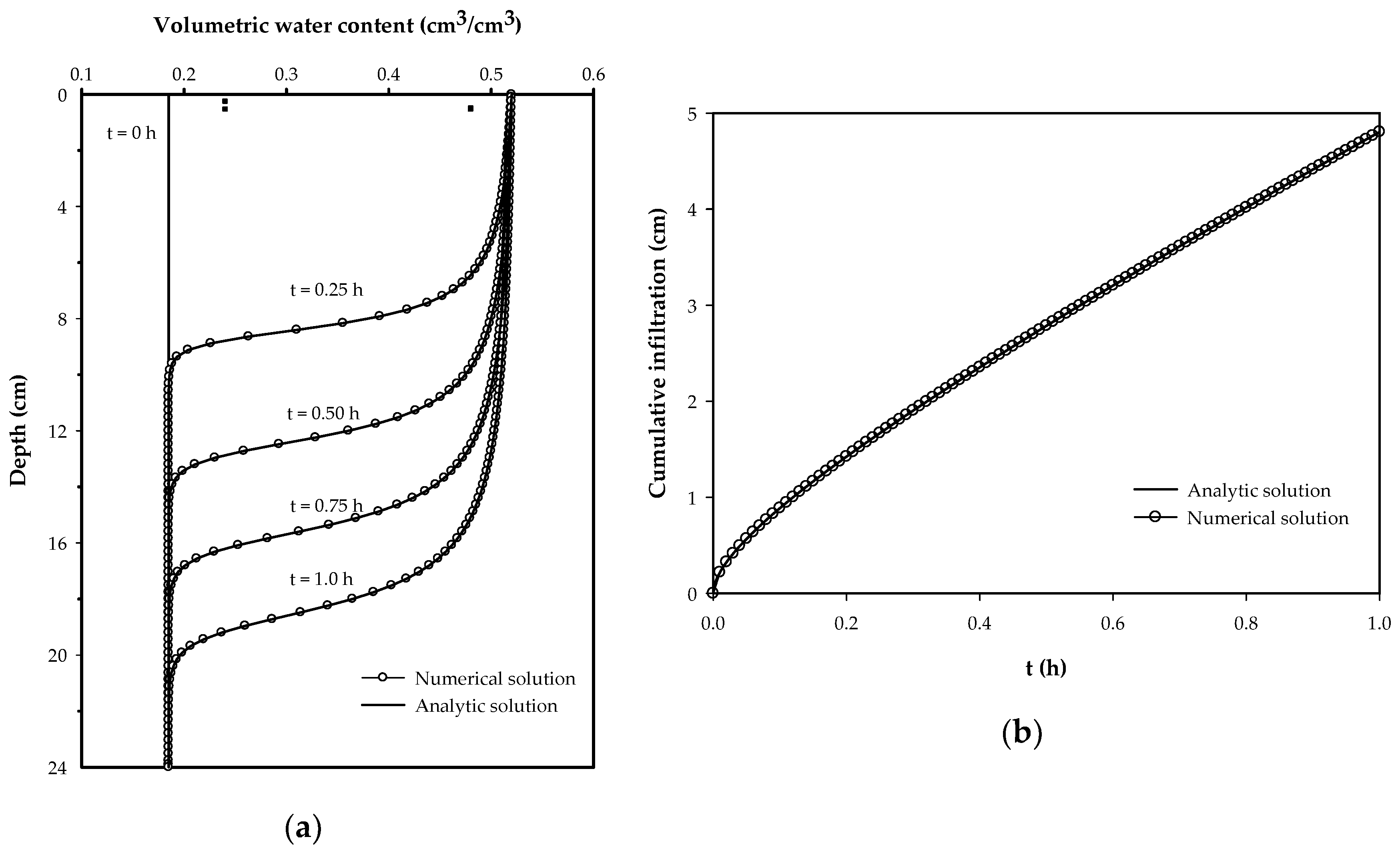
3.1. Comparison between Numerical and Analytical Solutions

A comparison between the numerical solution and analytical solution was carried out in the soil of Montecillo, State of Mexico, the American textural classification of which is a sandy loam soil; the soil was characterized hydrodynamically via the internal drainage method [19]. According to Fuentes et al. [20], the values of the parameters of the Fujita and Parlange characteristics are θ_s = 0.520 cm³/cm³, θ₀ = 0.185 cm³/cm³, $\left|{\mathsf{\psi }}_{\mathrm{c}}\right|$ = 13.500 cm, $\left|{\mathsf{\psi }}_{\mathrm{s}}\right|$ = 0.000 cm, K_s = 2.5 cm/h, K₀ = 0.000 cm/h, α = 0.969, and β = 0.998.

Of the behavior in short time periods of the infiltration solution under the conditions studied, a relationship between space and time steps can be deduced. In short time periods, I = S$\sqrt{\mathrm{t}}$, so in the first time step, I ≈ ∆z∆θ and t = ∆t, where ∆θ = θ_s − θ₀; since S² ≈ 2 (K_s − K₀) λ_c∆θ, the time and space steps must be such that the dimentionless parameter is of the order of unity [17].

$$\mathrm{m}=\frac{2\left({\mathrm{K}}_{\mathrm{s}}-{\mathrm{K}}_0\right){\mathsf{\lambda }}_{\mathrm{c}}}{\Delta \mathsf{\theta }}\frac{\Delta \mathrm{t}}{{\left(\Delta \mathrm{z}\right)}^2}$$

(49)

The comparison between the numerical solution of finite differences of the Richards equation and the analytical solution of Parlange [13] is shown in Figure 2. The results are similar if the parameter interpolator in time ($\mathsf{\omega }$) is close to unity, that is, if the scheme is fully implicit. The convergence of the numerical scheme and its stability are discussed in depth elsewhere [21].

3.2. Simulations under Different Boundary Conditions

Numerical simulations of infiltration, redistribution, and evaporation of water in a soil column in Montecillo, State of Mexico were performed using the hydrodynamic characteristics of van Genuchten [14] for the retention curve and those of Brooks and Corey [16] for the hydraulic conductivity curve. The retention curve proposed by van Genuchten is written as

$$\frac{\mathsf{\theta }\left(\mathsf{\psi }\right)-{\mathsf{\theta }}_{\mathrm{r}}}{{\mathsf{\theta }}_{\mathrm{s}}-{\mathsf{\theta }}_{\mathrm{r}}}={\left[1+{\left(\frac{\mathsf{\psi }}{{\mathsf{\psi }}_{\mathrm{d}}}\right)}^{\mathrm{n}}\right]}^{-\mathrm{m}}$$

(50)

where θ_s is the volumetric water content at saturation, θ_r is the volumetric content of residual water, ψ_d is a characteristic value of the water pressure in soil, and m and n are two parameters of empirical shape related here by the Burdine restriction [15]: m = 1 − 2/n, with 0 < m < 1 and n > 2.

The hydraulic conductivity proposed by Brooks and Corey is

$$\mathrm{K}(\mathsf{\theta })={\mathrm{K}}_{\mathrm{s}}{\left(\frac{\mathsf{\theta }-{\mathsf{\theta }}_{\mathrm{r}}}{{\mathsf{\theta }}_{\mathrm{s}}-{\mathsf{\theta }}_{\mathrm{r}}}\right)}^{\mathsf{\eta }}$$

(51)

where $\mathsf{\eta }$ is a parameter of positive form.

According to the methodology proposed by Fuentes [22], the parameters θ_s, θ_r, m, and $\mathsf{\eta }$ of Equations (50) and (51) were estimated from the porosity and granulometric curve and parameters Ks and ψ_d by applying an inverse parameter estimation method using advance phase data in an irrigation test and the Barré de Saint-Venant [4] and Richards [5] equations, in a border with a sandy loam soil in Montecillo, Mexico. The values were θ_s = 0.4865 cm³/cm³, θ_r = 0.0 cm³/cm³, m = 0.125, n = 2.2857, η = 11.0, ψ_d = −32.75 cm, and K_s = 1.84 cm/h.

The water content at the permanent wilting point (θ_PMP) and field capacity (θ_CC) were estimated as corresponding to water pressure ψ_PMP = −15,300 cm and ψ_CC = −340 cm, respectively, as follows: θ_PMP = 0.0840 cm³/cm³ and θ_CC = 0.2492 cm³/cm³. The initial moisture content at which soil irrigation must be carried out was calculated as θ₀ = θ_PMP + F_ap (θ_CC − θ_PMP), where F_ap is the permissible depletion factor of the crop, for example, F_ap = 1/3; using the above values, we obtained θ₀ = 0.1391 cm³/cm³. The water pressure on the surface was taken to be equal to the average, h = 1.5 cm. The net water depth of irrigation was calculated as (θ_CC − θ₀)/P_r, where P_r is the thickness of the considered soil profile; for a depth of 70 cm, the net water depth is 7.71 cm, which corresponds to an application efficiency of 83.3% to a gross water depth of 9.25 cm, which is applied in an irrigation time of 86 min. Figure 3 shows the results of the numerical simulations.

3.3. Evaporation and Transpiration Processes

Immediately after irrigation, processes of water redistribution due to the gravitational field, water consumption by plants, or transpiration and evaporation through the soil surface are started. For purposes of illustration, the evaporation process was simplified and represented by the following harmonic describing its variation in time:

$${\mathrm{e}}_{\mathrm{v}}\left(\mathrm{t}\right)={\overline{\mathrm{e}}}_{\mathrm{v}}+{\mathrm{c}}_{\mathrm{v}}\cos \left[\mathsf{\omega }\left(\mathrm{t}-{\mathrm{t}}_{\mathrm{M}}\right)\right];\mathsf{\omega }=\frac{2\pi }{\mathrm{P}}$$

(52)

where $\mathsf{\omega }$ is the angular frequency, P = 24 h is the period, $\overline{{\mathrm{e}}_{\mathrm{v}}}$ is the evaporated water depth hourly mean, ϕ = −ω${\mathrm{t}}_{\mathrm{M}}$ is the phase angle, ${\mathrm{t}}_{\mathrm{M}}$ is the time at which the hourly evaporation reaches its maximum value ${\mathrm{e}}_{\mathrm{vM}}={\mathrm{e}}_{\mathrm{v}}\left({\mathrm{t}}_{\mathrm{M}}\right)$, and ${\mathrm{c}}_{\mathrm{v}}={\mathrm{e}}_{\mathrm{vM}}-\overline{{\mathrm{e}}_{\mathrm{v}}}$. The minimum value is ${\mathrm{e}}_{\mathrm{vm}}=\overline{{\mathrm{e}}_{\mathrm{v}}}-{\mathrm{c}}_{\mathrm{v}}$; therefore, ${\mathrm{e}}_{\mathrm{vm}}+ {\mathrm{e}}_{\mathrm{vM}}=2\overline{{\mathrm{e}}_{\mathrm{v}}}$ is satisfied.

To calculate the parameters of the harmonic, it was considered that the average annual water depth evaporated is Ev_a = 1,168 mm, which provides average daily water depth Ev_d = 3.2 mm/d and hourly mean water depth $\overline{{\mathrm{e}}_{\mathrm{v}}}$ = 0.13 mm/h. The selection of ${\mathrm{e}}_{\mathrm{vm}}$ = 0 mm/h leads to ${\mathrm{e}}_{\mathrm{vM}}$ = 0.27 mm/h. If the origin of time is taken at midnight, then ${\mathrm{t}}_{\mathrm{M}}$ = 15 h can be taken as the time where the hourly evaporation rate is the highest. Evaporation as a boundary condition was introduced as a Neumann condition in the upper boundary, making ${{\mathrm{q}}_{\mathrm{z}}|}_1^{\mathrm{k}+1}$ = −e_v (t_k + 1).

For transpiration, there are different possibilities, such as the models that include root density or laws of type Ohm. For purposes of illustration, the sink term studied by Zataráin et al. [17] was taken, namely,

$$\mathsf{\Upsilon }=-\frac{\mathsf{\gamma }}{{\mathsf{\lambda }}_{\mathrm{c}}}\mathrm{K}\left(\mathsf{\psi }\right)\frac{\partial \mathsf{\psi }}{\partial \mathrm{z}}$$

(53)

where $\mathsf{\gamma }$ is a dimensionless coefficient reflecting the demand for water by the sink; γ = 0.015 was taken as an example. The Bouwer scale [15] is defined by

$${\mathsf{\lambda }}_{\mathrm{c}}=\frac{1}{{\mathrm{K}}_{\mathrm{s}}}{\displaystyle \underset{-\infty }{\overset{0}{\int }}\mathrm{K}\left(\mathsf{\psi }\right)\mathrm{d}\mathsf{\psi }}.$$

(54)

With the hydrodynamic characteristics defined by Equations (50) and (51), it is calculated as

$${\mathsf{\lambda }}_{\mathrm{c}}=\left|{\mathsf{\psi }}_{\mathrm{d}}\right|\frac{1}{\mathrm{n}}\mathrm{B}\left(\mathsf{\eta }\mathrm{m}-\frac{1}{\mathrm{n}},\frac{1}{\mathrm{n}}\right)$$

(55)

where B(p, q) = Γ(p) Γ(q)/Γ(p + q) is the complete beta function with p > 0 and q > 0, and Γ(x) is the complete Euler gamma function. For the sandy loam soil under study, λ_c = 33.95 cm.

Within the local balance scheme, the discrete form of Equation (53) is

$${\mathsf{\Upsilon }}_{\mathrm{j}}^{\mathrm{k}+\mathsf{\omega }}=-\frac{\mathsf{\gamma }{\mathrm{K}}_{\mathrm{j}}^{\mathrm{k}+\mathsf{\omega }}}{{\mathsf{\lambda }}_{\mathrm{c}}\Delta {\mathrm{z}}_{\mathrm{j}}}\left({\mathsf{\psi }}_{\mathrm{j}+{\mathsf{\gamma }}_{\mathrm{z}}}^{\mathrm{k}+\mathsf{\omega }}-{\mathsf{\psi }}_{\mathrm{j}-1+{\mathsf{\gamma }}_{\mathrm{z}}}^{\mathrm{k}+\mathsf{\omega }}\right)$$

(56)

where ${\mathrm{K}}_{\mathrm{j}}^{\mathrm{k}+\mathsf{\omega }}$ = K (${\mathsf{\psi }}_{\mathrm{j}}^{\mathrm{k}+\mathsf{\omega }}$). The interpolation defined by Equation (15) should be used and similar terms should be grouped as in system (16). Figure 4 shows the evolution of the moisture profile after irrigation, due to redistribution caused by the gravitational field, to evaporation through the soil surface, to transpiration by crops, and to percolation in the base of the control column of the sandy loam soil in Montecillo, Mexico. Figure 5 shows the evolution of the corresponding accumulated water depth as a function of time in the profile of the soil control. One month after irrigation, the average moisture content was $\overline{\mathsf{\theta }}$ = 0.2060 cm³/cm³, which should continue decreasing over time to achieve the average initial moisture content θ₀ = 0.1391 cm³/cm³ in order to apply the second irrigation.

4. Conclusions

A differential equation describing the transfer of water in soil was integrated analytically for a few initial and boundary conditions of practical interest, such as in a semi-infinite soil column with constant initial moisture content and constant moisture conditions at its upper boundary. In the general case, the integration is done in a numerical manner, which is why the numerical scheme was presented via the finite difference method.

Using the finite difference method, a scheme of local balance in one dimension of space was given. This scheme has the peculiarity that the coefficients involving specific capacity and hydraulic conductivity depend on the desired pressure in a given time step, making the resolution of the system of discrete equations occur via an iterative method. The presented solution was compared with the analytical solution, which permitted us to establish a relationship between the steps of time and space. The solutions are similar if the scheme is taken to be close to or equal to a fully implicit scheme.

Finally, with the numerical solution, we have a tool allowing us to know more about the evolution of the moisture profile and infiltrated water depth during irrigation and the evolution of the moisture profile after irrigation: the redistribution of moisture due to the gravitational field, evaporation of water through the soil surface, transpiration from plants with a simplified model of the sink term, and percolation. The use of the numerical solution helps us to understand the movement of water in an irrigation event, which allows us to give pertinent recommendations for the efficient application of water to a plot.

References

1. Fuentes, C.; De León-Mojarro, B.; Hernández-Saucedo, F.R. Gravity irrigation hydraulics. In Gravity Irrigation; Fuentes, C., Rendón, L., Eds.; Nacional Association of Irrigation Specialist: Mexico, Spain, 2017; pp. 1–66. [Google Scholar]
2. Chávez, C.; Fuentes, C. Design and evaluation of surface irrigation systems applying an analytical formula in the irrigation district 085, La Begoña, Mexico. Agric. Water Manag. 2019, 221, 279–285. [Google Scholar] [CrossRef]
3. Morbidelli, R.; Corradini, C.; Saltalippi, C.; Flammini, A.; Dari, J.; Govindaraju, R.S. Rainfall Infiltration Modeling: A Review. Water 2018, 10, 1873. [Google Scholar] [CrossRef] [Green Version]
4. Saint-Venant, A.J.C.; Barre, D. Théorie du mouvement non permant des eaux, avec application aux crues des rivières et à l’introduction des marées dans leur lits. C. R. Séances l’Academie Sci. 1871, 73, 147–154, 237–240. [Google Scholar]
5. Richards, L.A. Capillary conduction of liquids through porous mediums. Physics 1931, 1, 318–333. [Google Scholar] [CrossRef]
6. Parlange, J.Y. On solving the flow equation in unsaturated soils by optimization: Horizontal infiltration. Soil Sci. Soc. Am. Proc. 1975, 39, 415–418. [Google Scholar] [CrossRef]
7. Saucedo, H.; Zavala, M.; Fuentes, C. Complete hydrodynamic model for border irrigation. Water Technol. Sci. 2011, 2, 23–38. [Google Scholar]
8. Saucedo, H.; Zavala, M.; Fuentes, C.; Castanedo, V. Optimal flow model for plot irrigation. Water Technol. Sci. 2013, 4, 135–148. [Google Scholar]
9. Saucedo, H.; Fuentes, C.; Zavala, M. The Saint-Venant and Richards equation system in surface irrigation: 2) Numerical coupling for the advance phase in border irrigation. Ing. Hidraul. Mex. 2005, 20, 109–119. [Google Scholar]
10. Darcy, H. Dètermination des lois d’ècoulement de l’eau à travers le sable. In Les Fontaines Publiques de la Ville de Dijon; Dalmont, V., Ed.; Victor Dalmont: Paris, France, 1856; pp. 590–594. [Google Scholar]
11. Fuentes, C.; Haverkamp, R.; Parlange, J.Y. Parameter constraints on closed–form soil-water relationships. J. Hydrol. 1992, 134, 117–142. [Google Scholar] [CrossRef]
12. Fujita, H. The exact pattern of a concentration-dependent diffusion in a semi-infinite medium, part II. Text. Res. J. 1952, 22, 823–827. [Google Scholar] [CrossRef]
13. Parlange, J.Y.; Braddock, R.D.; Lisle, I.; Smith, R.E. Three parameter infiltration equation. Soil Sci. 1982, 111, 170–174. [Google Scholar] [CrossRef]
14. Van Genuchten, M.T. A closed-form equation for predicting the hydraulic conductivity of unsaturated soils. Soil Sci. Soc. Am. J. 1980, 44, 892–898. [Google Scholar] [CrossRef] [Green Version]
15. Burdine, N.T. Relative permeability calculation from size distributions data. Trans. AIME 1953, 198, 171–199. [Google Scholar]
16. Brooks, R.H.; Corey, A.T. Hydraulic properties of porous media. In Hydrology Papers; Colorado State University: Colorado, CO, USA, 1964; Volume 3. [Google Scholar]
17. Zataráin, F.; Fuentes, C.; Palacios, V.O.L.; Mercado, E.J.; Brambila, F.; Villanueva, N. Modelación del transporte de agua y de solutos en el suelo. Agrociencia 1998, 32, 373–383. [Google Scholar]
18. Bouwer, H. Rapid field measurement of air entry value and hydraulic conductivity of soil as significant parameters in flow system analysis. Water Resour. Res. 1964, 36, 411–424. [Google Scholar] [CrossRef]
19. Cano, M.A. Caracterización Hidrodinámica del Suelo in Situ y Cálculo de Percolación y Evapotranspiración en Riego por Goteo. Master’s Thesis, Centro de Hidrociencias del Colegio de Postgraduados, Montecillo, Texcoco, México, 1990. [Google Scholar]
20. Fuentes, C.; Chávez, C.; Saucedo, H.; Zavala, M. On an exact solution of the non-linear Fokker-Planck equation with sink term. Water Technol. Sci. 2011, 2, 117–132. [Google Scholar]
21. Chávez, C.; Antonino, A.C.D.; Fuentes, C. Numerical solution of the infiltration equation. In Gravity Irrigation; Fuentes, C., Rendón, L., Eds.; Nacional Association of Irrigation Specialist: Mexico, 2017; pp. 215–252. [Google Scholar]
22. Fuentes, C. Approche Fractale des Transferts Hydriques dans les sols non Saturès. Ph.D. Thesis, de la Universidad Joseph Fourier de Grenoble, Grenoble, France, 1992; p. 267. [Google Scholar]
Figure 1. The domain resolution of the Richards equation; ω is the is the interpolation factor in time and γ is the interpolation factor in space.
Mathematics 08 01581 g001
Figure 2. Moisture profiles (a) and cumulative infiltration (b) obtained via numerical and analytical solutions of infiltration in sandy loam soil of Montecillo, Mexico.
Mathematics 08 01581 g002
Figure 3. Water infiltration during the first irrigation in sandy loam soil in Montecillo, Mexico.
Mathematics 08 01581 g003
Figure 4. Water redistribution after one irrigation in the profile of the sandy loam soil in Montecillo, Mexico.
Mathematics 08 01581 g004
Figure 5. Accumulated water tables as a function of time in the soil control profile, evaporated, transpired, and percolated after irrigation in sandy loam soil in Montecillo, Mexico.
Mathematics 08 01581 g005