Abstract
A version of the central limit theorem is proved for sums with a random number of independent and not necessarily identically distributed random variables in the double array limit scheme. It is demonstrated that arbitrary normal mixtures appear as the limit distribution. This result is used to substantiate the log-normal finite mixture approximations for the particle size distributions of the lunar regolith. This model is used as the theoretical background of the two different statistical procedures for processing real data based on bootstrap and minimum estimates. It is shown that the cluster analysis of the parameters of the proposed models can be a promising tool for revealing the structure of such real data, taking into account the physico-chemical interpretation of the results. Similar methods can be successfully used for solving problems from other subject fields with grouped observations, and only some characteristic points of the empirical distribution function are given.
Keywords:
central limit theorem; random sequence; random index; transfer theorem; random sum; random Lindeberg condition; log-normal mixtures; grouped data; bootstrap; minimizing χ2 estimate; EM algorithm; statistical estimations MSC:
60F05; 62N01; 65C20; 85-08
1. Introduction
The study of regularities in the sizes of particles of lunar and other planetary regoliths is relevant for planning and design of manned and unmanned space missions for exploration of space bodies such as the Moon, asteroids, planets, and their satellites. In the conditions of low gravity and the absence of dense atmosphere, dust structures acquire properties that are not typical for Earth conditions: they form clouds of charged particles that have very high abrasive properties. They deposit on structural elements of stations and spaceships, e.g., on solar batteries, and space suites causing their malfunction and failures. Thus, the solution of the problem under consideration may turn very useful and prospective in the preparation of new space missions to increase their safety and general success.
In the present paper, we consider the problem of modeling the distribution of the sizes of dust particles in the lunar regolith formed as a result of multiple impacts, e.g., of the bombardment of the lunar surface by meteorites. These impacts are accompanied by both processes of explosion dispersion of particles with their fragmentation and processes of the agglomeration of particles in exothermic plasma-chemical synthesis reactions [1]. As it was noted in the book [2], the observed statistical distributions of the particle size in lunar regolith, as a rule, have heavy power-type tails.
In this paper, we combine and generalize the results of the papers [3,4] in order to obtain a general model of the particle size distribution that can be applied to describe statistical regularities in the lunar regolith probes brought by the Apollo missions. The proposed models have the form of asymptotic approximations obtained by a central limit theorem for sums of a random number of independent not necessarily identically distributed random variables in the special double array limit scheme.
Some words about the history of the problem. Initially, the studies of these models concerned pure fragmentation of particles related to mining processes. In the paper [5] by N. K. Razumovsky published in 1940, many cases were described where the logarithms of the particle sizes (e.g., of gold grains or ore particles under crushing) had approximately normal (Gaussian) distribution. This paper attracted the attention of A. N. Kolmogorov who suggested a mathematical model that analytically explained the appearance of the log-normal distribution of the particle size under crushing, as well as minerals in geological samples [6]. The mathematical model suggested by Kolmogorov was based on the study of the change of the number of particles, whose size does not exceed a specified threshold, in time. Kolmogorov’s result is valid under rather strong assumptions. In particular, within the framework of Kolmogorov’s model, for the distribution of particle size under crushing to be log-normal, it is necessary that the crushing rate is constant, that is, does not depend on the current sizes of the crushed particles. At the same time, it is practically obvious that, as the particle (grain) becomes smaller, the intensity of its collisions with other particles (grais) or elements of the crusher may change, e.g., decrease by virtue of the fact that the probability of a collision of the particle with other particles is in some sense proportional to the particle size so that, the smaller the particle, the less is this probability. This circumstance was noted by Kolmogorov himself, who wrote in the final part of his paper [6]: “It would be interesting to study mathematical schemes in which the crushing rate decreases (or increases) with the decrease of their sizes. As this is so, first of all, it is natural to consider the cases where the crushing rate is proportional to some power of the particle size. If this power differs from zero, then, apparently, the log-normal law will not be applicable”. In the paper [7], the results of statistical analysis of real data were presented that confirmed the log-normal model for the distribution of the sizes of grains in rock formations.
However, some works contain empirical evidence that sometimes the log-normal model for the distribution of particle size under crushing is not adequate. As far back ago as in 1954, R. A. Bagnold in his book [8] noticed that the logarithm of the probability density function of the logarithm of the particle size in natural sand deposits resembles a hyperbola rather than a parabola. This means that, in accordance with Bagnold’s observations, the particle size distribution possesses exponentially decreasing tails rather than log-normal.
This circumstance induced some specialists to pay attention to such models as log-asymmetric Laplace distribution, the so-called two-sided Pareto-log-normal distribution or log-normalinverse Gaussian (NIG) distribution. In particular, in [9,10], the models were considered for the process of forming of the particle size distribution under crushing based on the assumption that, while moving from one place to another, a particle can be split into some smaller particles as a result of collisions or other impacts implying the randomness of the particle mass after splitting. The particles do not reach the terminal point simultaneously. Some of them can change the direction of their motion or stick for a long time while others can pass their way much sooner without collisions. The state of a particle obviously depends on its distance from the terminal point. The Reed–Jorgensen and Sørensen models take this realities into account by assuming that the time the particle is observed at is random. Actually, Reed, Jorgensen and Sørensen introduced randomization into the model suggested by Kolmogorov in 1941, by assuming that it takes different times for different particles to move from one source to another.
In the Reed–Jorgensen model, the time from the start of the particle’s motion to its “termination” is assumed to be an exponentially distributed random variable, so that the final particle size distribution turns out to be two-sided Pareto-log-normal.
Probability distributions for which the logarithm of the density function is a hyperbola (hyperbolic distributions) were introduced by O.-E. Barndorff-Nielsen in 1977 [11]. In several papers, it was noted that hyperbolic distributions demonstrated high concordance with empirical distributions of real geological data; see, e.g., [12,13,14]. Actually, in Ref. [11], a more general class of probability distributions was introduced, the class of so-called generalized hyperbolic distributions. The NIG distribution is a representative of this class. By definition, this distribution is a special (variance-mean) mixture of normal distribution, the mixing distribution being inverse Gaussian. The NIG distribution demonstrates even better fit to empirical distributions of the logarithm of particle size than the hyperbolic distribution. This is due to that the tails of NIG distributions are heavier than those of the “ordinary” hyperbolic distribution, as is typical, say, for the natural sand deposits. Another advantage of the NIG distributions is that they possess many favorable mathematical properties. For example, their moments can be calculated explicitly.
In the Sørensen model, the motion of the particle is assumed Brownian. Therefore, the time from the start of the motion to its termination is random with the inverse Gaussian distribution. This results in the logarithm of the particle size having the NIG distribution.
The Reed–Jorgensen and Sørensen models demonstrate very good fit to the empirical data of particle (grain) sizes in natural deposits. However, these models do not take into account Kolmogorov’s remark: in these models, the crushing intensity remains constant.
In Ref. [3], a more general model was considered within which the crushing intensity could be variable and even random. In [3], the process of relative changes of the particle size was assumed to be compound doubly stochastic Poisson process, and it was demonstrated that the randomness of the intensity of the crushing process might lead to the particle size distribution having the form of a mixture of log-normal distributions. In accordance with such a model, the distribution of the number of size changes prior to any observation time is mixed Poisson. As it was noted in [15], these processes are natural models of non-stationary chaotic stochastic processes possessing some extremal entropy properties. It should be mentioned that in the Reed–Jorgensen and Sørensen models, a homogeneous Poisson point process was considered as a model of the flow of events implying the changes of the particle size.
As it has been already noted, in all the works mentioned above, the process of pure fragmentation of particles was considered so that every impact of particles could result in a decrease of their sizes only, whereas, in plasma-chemical reactions in the regoliths on the surface of space bodies devoid of dense atmospheres, every impact can result in both decrease and increase of the particle size, say, due to sintering. In the present paper, we consider models for the particle size distribution that take this circumstance into account. Unlike Kolmogorov’s approach where the main object of study was the number of particles with a certain size, here we consider the evolution of the size of a separate particle.
One more characteristic feature of the models considered in the present paper is their generality. All the models mentioned above have the form of special mixtures of log-normal distributions: the Reed–Jorgensen, Sørensen, and Barndorff–Nielsen models have the form of normal variance–mean mixtures. In these mixtures, the scale and location parameters of the mixed distributions are rigidly bound so that actually mixing is performed with respect to one parameter. This construction noticeably complicates the physical interpretation of the obtained models. In the present paper, we propose a rather realistic scheme of forming of models that are general mixtures of log-normal models in which the mixing distribution is, in general, two-variate. Although these models seem to be too general so that the statistical estimation of the distributions can be very complicated, they allow natural discrete approximations for the mixing distributions. In this case, the approximate model for the particle size distribution is a finite mixture of log-normal distributions, whose parameters can be estimated by standard statistical procedures of the EM-algorithm type.
The paper is organized in the following way. Section 2 contains the description of the mathematical foundation of general normal mixture models for the particle size distribution. We formulate a new general version of the central limit theorem for random sums in a special double array limit scheme stating that, under rather general and reasonable random Lindeberg condition, the distribution of the sum of a random number of independent random variables with finite second moments approaches the set of normal location-scale mixtures, so that, within this set, a mixture can be chosen that can be used as an asymptotic approximation to the distribution of the random sum. This result is used in Section 3 as the base for the main model of the particle size distribution. In Section 4, we discuss the approximation of the sample distribution function constructed from data given in the NASA catalog [16] by the method of statistical simulation of samples by the bootstrap technique. In Section 5, we discuss the approximation of the sample distribution function by the minimization of the statistic. In Section 6, we use the cluster analysis to separate some typical regularities in the parameters of distributions fitted to all 317 samples of lunar regolith presented in the NASA catalog [16]. The obtained results demonstrate that the finite normal mixture model fits the real data very well measured in both the classical metric scale (micrometers, m) and scale conventional in geology and selenology [17]. Appendix A contains the description of the algorithms used for the approximation of the distribution of particle size in lunar regolith by finite normal mixtures. Appendix B presents figures that demonstrate application of proposed algorithms for lunar regolith samples.
2. Central Limit Theorem for Sums of a Random Number of Independent Not Identically Distributed Random Variables in the Special Double Array Limit Scheme
Assume that all the random variables considered in this paper are defined on one and the same probability space . The symbols and ⟹ will denote coincidence of distributions and weak convergence (convergence in distribution).
Let and be a double array of random variables, and are real numbers, . The row-wise independence of is not assumed. Consider a family of the random variables
with characteristic functions , . Consider a family of nonnegative integer-valued random variables such that, for each , the random variables and are independent. Let Y be a random variable with distribution and characteristic function and , , respectively.
Definition 1
([4]). The random variables and Y are said to satisfy the coherency condition, if, for any ,
It is worth noting that, if row-wise convergence to Y takes place, the relation
holds for any and . Thus, we can say that coherency condition (2) means that “pure” row-wise convergence (3) takes place “on the average” so that the “row-wise” convergence as is somehow coherent with the “principal” convergence as . Following [4], below we will deal with the case where the random variables have the additive structure and are formed as sums of independent random variables with the finite second moment. It turns out that, under these additional “structural” assumptions, the role of coherency condition is played by the “random Lindeberg condition”. Furthermore, if we deal not with a double array of random variables but simply with a sequence of random variables, then, as was shown in [18,19], the coherency condition turns out to be equivalent to the following set of conditions: the indices infinitely increase in probability that is as for any , and either or as .
Let and be real numbers, . Denote
Let , be a double array of row-wise independent not necessarily identically distributed random variables with distribution functions . Denote
The following statement is actually a transfer theorem for the double array limit scheme under consideration.
Lemma 1
([4]). Assume that coherency condition (2) holds. If there exist random variables U and V such that the joint distributions of the couples converge to that of the couple as , then
as , where the random variable Y is independent of the couple .
It follows from Lemma 1 that the distribution and characteristic functions of random variables Z and Y are related as
that is, the limit law for normalized randomly indexed random variables is a scale-location mixture of the distributions, which are limiting for normalized non-randomly indexed random variables .
For fixed random variables Z and Y, introduce the set containing all couples of random variables such that the characteristic function can be represented in the form (6) and . Whatever random variables Z and Y are, the set is always nonempty since it trivially contains the couple . The set may contain more than one element. For example, if Y is the standard normal random variable and where and are independent random variables with the same standard exponential distribution, then, along with the couple , the set contains the couple . In this case, is the symmetric Laplace distribution.
Definition 2
([20]). A family of random variables is said to be weakly relatively compact, if each sequence of its elements contains a weakly convergent subsequence. In the finite-dimensional case, the weak relative compactness of a family is equivalent to its tightness:
Let be any probability metric which metrizes weak convergence in the space of two-dimensional random vectors, for example, the Lévy–Prokhorov metric [21].
Lemma 2
([4]). Assume that the random variables have the form (4). Let the family of random variables be weakly relatively compact. Assume that coherency condition (2) holds. Then, convergence (5) of normalized random sums to some random variable Z takes place with some if and only if there exists a weakly relatively compact sequence of couples , , such that condition
holds.
Denote , and assume that , . Denote
It is easy to make sure that , , . In order to formulate a version of the central limit theorem for random sums with the limiting distribution being an arbitrary normal mixture, assume that non-random sums, as usual, are centered by their expectations and normalized by by their mean square deviations and put , , . As this is so, as and we can (but are not obliged to) take and , respectively.
Now let Y be a random variable with the standard normal distribution:
Theorem 1.
Assume that the random Lindeberg condition holds: for any ,
Proof.
We will deduce Theorem 1 from Lemma 2. First, check that, in the case under consideration, the family of random variables is weakly relatively compact. For , by the Chebyshev inequality, we have
as , that is, the family is tight and hence weakly relatively compact.
Second, exactly in the same way as it was done in the proof of Theorem 4 in [4], it can be proved that the random Lindeberg condition (8) implies the coherency condition (2) with being the characteristic function of the standard normal distribution, , .
Thus, Theorem 1 becomes a simple consequence of Lemma 2. □
Actually, Theorem 1 means that, under a rather general and reasonable random Lindeberg condition, the distribution of the sum of a random number of independent random variables with finite second moments approaches the set of normal location-scale mixtures, so that, with finite n, within this set, a mixture can be chosen that can be used as an asymptotic approximation to the distribution of the random sum.
Theorem 1 is a substantial generalization and strengthening of a result of [22] where a special version of the random Lindeberg condition was used with geometrically distributed random variables to establish sufficient conditions of convergence of the distributions of random sums to the Laplace law. In turn, Ref. [22] was not the first work where the random Lindeberg condition was used. Apparently, it was introduced in [23], where several equivalent formulations of this condition were presented. In [24], it was proved that, under some additional assumptions, the random Lindeberg condition is necessary and sufficient for the convergence of the distributions of randomly centered random sums to the normal distribution. Here, we consider a case significantly more general than those considered in [24] or [22].
Since, unlike one-parameter normal mixtures (pure scale mixtures, pure location mixtures, variance–mean mixtures), two-parameter normal scale-location mixtures are not identifiable, in Theorem 1 condition (7) describing the rapprochement of the sequence of couples of the random variables with the special set of couples in Theorem 1 cannot be replaced by a condition of convergence of this sequence to an element of this set so that the ‘if and only if’ character of Theorem 1 was preserved. However, the latter condition (which is obviously stronger than (8)) together with the random Lindeberg condition are sufficient for the convergence (5). Namely, the following transfer theorem holds concretizing Lemma 1.
Corollary 1.
Assume that the random Lindeberg condition (8) holds and there exist , and a couple of random variables such that, as
Then, as ,
For , denote , , . In [4], it was demonstrated that, if the third absolute moments of the summands exist, then the random Lindeberg condition (8) follows from the random Lyapunov condition
which seems to be more easily verifiable than the random Lindeberg condition.
3. Mixed Log-Normal Models for the Distribution of the Particle Size
Although in this paper we will follow the general reasoning of [3], here we will use a scheme that is more general than that considered in [3]. The initial size of a particle (say, at some time instant to which, for convenience, we will assign that the value ) will be denoted . As time goes by, the particle undergoes collisions with other particles or other transformations due to heating, impacts with meteoroids, etc. We assume that the ith collision (transformation) results in the fact that, after it, the particle size becomes times that of its size before the ith transformation. Let be the number of transformations of the particle by time t. Then, the particle size at time t has the form . Hence,
where and .
In [3], it was assumed that are independent and identically distributed with . The assumptions of the coincidence of the distributions of are too restrictive since different collisions or transformations may be caused by processes of different types, say, fragmentation or agglomeration. Instead, here we will not impose such a condition.
As a theoretical foundation of the models proposed here, we will use the limit scheme that was considered in the preceding section and for the sake of generality introduce an auxiliary formal parameter and assume that, instead of one sequence of independent random variables , we will consider a double array , , of row-wise independent not necessarily identically distributed random variables. As above, we use the notation for the sum , .
Instead of a single counting process , now we will have a sequence of counting processes , so, instead of basic structural model (9), we will deal with the more general model . Fix the ‘terminal’ time and assume that for any so that, by definition, and
Model (11) can be interpreted in the following way. For a fixed n, the sequence describes a possible trajectory of the process of changes of the particle size. Actually, we are interested in the asymptotic approximation for the distribution of the ‘terminal’ size (4) with large (with large T or with a large intensity of transformations). Having introduced the auxiliary (infinitely large) parameter n, we obtained the possibility to consider the scheme within which it is admitted that, as n changes, the distributions of can also change as if, instead of a single particle, we deal with a set of particles with ‘long and possibly different histories’. As this is so, each trajectory starts with its own initial size so that
As in Section 2, denote , and assume that , . In all the preceding papers, pure fragmentation (crushing) was considered, and it was assumed that resulting in . The equality of to zero corresponded to the case of ‘degenerate’ fragmentation leaving each particle unchanged. In the present paper, the parameters can be both positive and negative. The case corresponds to fragmentation, whereas the case corresponds to agglomeration.
The assumption is not superfluously restrictive. From the practical point of view, this assumption actually withdraws beyond the range of considered cases only those situations that admit either instantaneous zeroing of the particle size or, vice versa, instantaneous increase of the size of a small particle to very large (infinitely large) values. As one more argument in favor of the assumption of finiteness of the second moment of the random variables , note that stable laws are well-known examples of distributions with very heavy tails decreasing as power functions with a small exponent. However, even their logarithmic moments are finite.
Based on Theorem 1, we can conclude that, under very general conditions, the approximation to the distribution of the logarithm of the particle size should be sought within the family of normal scale-location mixtures. In other words, the approximation to the distributions of the particle size itself should be sought within log-[normal scale-location mixtures,] that is, if Z is the particle size, then
for some couple of random variables . It can be easily seen that the log-[normal scale-location mixture] on the right-hand side of (12) is actually the scale-location mixture of log-normal distributions.
Furthermore, from the definition of the Lebesgue integral, it follows that any normal scale-location mixture can be approximated by a finite normal scale-location mixture, that is, in practice, the approximations to the distribution of the particle size can be sought in the form
with some , , , , , . Finite normal mixture model (13) is more convenient and in some sense more interpretable since it allows for naturally separating some typical regularities in the data by well-known methods of statistical analysis, say, by the EM algorithm. It should be noted that the approximation of the general normal mixture by a finite mixture (13) is a kind of regularization of the originally ill-posed problem of estimation of the parameters of an unidentifiable general normal mixture, whereas finite normal mixtures are identifiable, that is, the problem of estimation of their parameters has a unique solution [25].
In what follows, we use model (13) to trace some statistical regularities in the particle sizes in the the probes of lunar regolith.
4. Approximation of a Sample Distribution Function Based on Sample Simulation
In the NASA catalog [16], the data are presented in the tabular form as the pairs “particle size–percentage of particles of this size in the sieved samples”. Information is available only on a few (as a rule, no more than ten) points of growth (selected, generally speaking, haphazardly) of the empirical distribution function, but there are no data between these points. In the original paper [16], Steineman’s interpolation [26] was used to approximate the distributions, and then the corresponding histograms were built using the macros of the Excel.
In this paper, piecewise cubic Hermite interpolating polynomials (see, for example, [27]) are used for similar purposes. They allowed us to obtain the curves that are closest to those presented in the NASA catalog.
The proposed approximation by Hermite polynomials made it possible to obtain a continuous empirical distribution function (ECDF) that allows for using the method of inverse transform sampling. The sample size for the estimation of the parameters was 10,000 observations. In addition, to test the homogeneity hypotheses concerning the coincidence of the approximating mixture and the original empirical distribution function by the one-sample Kolmogorov–Smirnov goodness-of-fit test, one more independent sample of 2500 observations was generated. In general, this procedure is methodically close to bootstrap. Its description is given in Algorithm A1.
The generated samples are used to obtain maximum likelihood estimates for the parameters of the approximating distribution (13) by the EM-algorithm for finite normal moxtures [28]. Some examples of applying this bootstrap procedure to real samples of the lunar regolith are shown on Figure A1, Figure A2, Figure A3, Figure A4, Figure A5, Figure A6, Figure A7, Figure A8 and Figure A9.
The graphs on the left show the initial data obtained in the sifting process from the tables of the NASA catalog (squares), their interpolation using Hermite polynomials (blue solid line), and the approximating mixture (magenta line). It is seen that both curves coincide almost everywhere. This situation is typical for the vast majority of analyzed samples. It is worth noting that several values were checked for the number k of components in (13). It was empirically found that the necessary balance between the quality of the approximation and the computational complexity is achieved at the value , which was further used to process all 317 samples.
The graphs on the right on Figure A1, Figure A2, Figure A3, Figure A4, Figure A5, Figure A6, Figure A7, Figure A8 and Figure A9 demonstrate the histograms for the simulated samples and sifted data constructed from ECDF for a particular sample, as well as their approximation by the density of the mixture distribution. It should be noted that the accuracy of the approximation was determined by the comparison with the empirical distribution function, so that these graphs are only a more detailed illustration of the method. Obviously, both distribution functions and histograms are visually very close, even with the account of various peculiarities. It is clear that in each case the shape of the distribution is far from that of the Gaussian law.
Figure A10 shows the results of the Kolmogorov–Smirnov homogeneity test from the additionally simulated samples. For clarity, the standard significance levels 0.01 and 0.05 are demonstrated. The first one is exceeded by p-values for 84.5% samples (268 of 317), whereas the second one is exceeded in 70.7% cases (224 of 317). Thus, for the vast majority of bootstrap samples, fairly good approximation was obtained. It is also worth noting that the shape of histograms for the simulated samples is quite close to those obtained in the NASA catalog. This fact is a clear confirmation of the correctness of the approach used, since, as it has already been noted, functionally or statistically, the distance between these functions was not measured, since it was not used as a criterion.
5. Approximation of a Sample Distribution Function Based on Minimizing Statistics
In the preceding section, a fairly high level of goodness-of-fit was demonstrated between the probability distributions obtained using the bootstrap procedure and the sifting data of the lunar regolith samples. However, this method has a number of disadvantages. Firstly, it is imperative to interpolate points (the initial data from the NASA catalog). The method of interpolation can significantly affect the final results. Secondly, the generation of samples and their processing by the EM-algorithm takes a rather noticeable computational time that grows as the sample size increases. In this section, an alternative approach will be proposed, within which the initial grouped data are also approximated by functions that have the form of a finite log-normal mixtures, so that statistical simulation of samples is not required. This can improve the accuracy of the approximation, as well as reduce the computational complexity of data processing.
To find the parameters of the approximating function, it is required to minimize the distance between this curve and the known values (points) of the empirical distribution function. In the preceding section, it was noted that the best results were obtained for four-component mixtures, but this method can use a different value of the parameter k.
Thus, for the approximation, the function of the type (13) can be used, where , and for each of the parameters the constraints mentioned above are valid (see the end of Section 3). Then, the statistics has the form
where and are known sets of values and percentages in the total number for the corresponding particle sizes from the NASA catalog, and n is the number of nonzero differences . It is worth noting that there are duplicate values of in the original data, so it had to be taken into account during data processing. In (14), it is assumed that all are different.
To find the numerical estimates of the unknown parameters with the account of the constraints mentioned above, we used the solution of a nonlinear programming problem by the algorithm based on the interior-point optimization [29]. The quality of the approximation was estimated by substituting the value of the statistic with the optimal set of parameters into the distribution function with degrees of freedom that gave the corresponding p-value. This procedure is described in Algorithm A2.
Examples of the application of this algorithm to real samples of the lunar regolith are shown in Figure A11, Figure A12, Figure A13, Figure A14, Figure A15, Figure A16, Figure A17, Figure A18 and Figure A19. The graphs show the initial data from the tables of the NASA catalog, their interpolation by the Hermite polynomials (blue solid line), and the bootstrap procedure (red line), as well as the approximating mixture obtained by the method of minimization of the statistics (magenta line). Here, the coincidence of the curves obtained by the two methods is not necessary, since the majority of the attention is paid to the approximation of the set of initial points. The graphs show curves for the same number of components , and, for each of the methods, a different value can be used.
Figure A20 demonstrates the results of the test for (see formula (13)). The graphs show the standard significance levels 0.05 and 0.01. The significance level 0.05 for the test is exceeded by the p-values for 92.7% samples (294 of 317) when approximated by three-component mixtures and for 93.1% of samples (295 of 317) when approximated by four-component mixtures. The significance level 0.01 is exceeded by the p-values in 94.6% cases (300 of 317) when approximating by three-component mixtures and for 94% samples (298 of 317) in the case of four-component mixtures. In fact, the quality of the statistical approximation is the same for both and . This allows for using fewer parameters when solving the constrained optimization problem.
Thus, the disadvantages of the bootstrap methodology method can be overcome. The quality of the approximation in this case can be assessed as excellent. The only important point of this approach is finding the solution by conditional optimization that seriously depends on the initial approximation and can lead to incorrect results. Therefore, careful adjustment of the parameters is required, as well as the use of a series of runs to select the most successful values. The computational complexity of the proposed procedure is moderate. Therefore, multiple computations are possible.
6. Cluster Analysis of the Mixture Parameters in Approximations of the Lunar Regolith Particle Size Distributions
This section presents the results of cluster analysis of the parameters of the components of all approximating finite normal mixtures at once. In this case, for partitioning into clusters, a full set of parameters (mathematical expectations, standard deviations and weights) are used, as well as a trivial inverse transformation to go from the scale for sizes to metric (m). The corresponding is given in Algorithm A3.
Figure A21, Figure A22, Figure A23 and Figure A24 (top graphs) demonstrate the relationship between the mathematical expectation and standard deviation for the scale as well as m for both methods discussed above. The size and color intensity of the points correspond to their weights (see formula (13) and the color bar on the figures). These figures essentially clarify and refine the linear approximation proposed in [30] for this dependence, which, as can be seen from Figure A21, Figure A22, Figure A23 and Figure A24, turns out to be overly rude.
The two lower plots in each of Figure A21, Figure A22, Figure A23 and Figure A24 demonstrate the partition of the parametric space into six groups by the k-medoids and fuzzy c-means clustering (in this case, the solution is the cluster with the maximum membership value for this element among all possible) for the bootstrap procedure and the method based on the estimates. It is obvious that the solutions of both methods in each of the cases are quite close. It should be noted that the results of fuzzy clustering have slightly better reproducibility compared to medoids under reclustering. For the clusters obtained by both methods, weights were determined as the ratio of the number of parameters included in the given cluster to the total number of points. The results are presented in Table 1 where the rows are in decreasing order of the corresponding weights.

Table 1.
Cluster size ratios.
The resulting clusters can be used, for example, to correlate with the chemical compounds of samples or other characteristics of the regolith.
A different representation of Figure A21, Figure A22, Figure A23 and Figure A24 is also possible, namely a three-dimensional image. In this case, the weights of the points are plotted on a separate scale, but their size when drawing is still determined by this parameter. Examples for each of the methods for metric and scales are shown in Figure A25, Figure A26, Figure A27 and Figure A28.
7. Conclusions
A version of the central limit theorem was proved for sums with a random number of independent and not necessarily identically distributed random variables in the double array limit scheme. It is demonstrated that arbitrary normal mixtures appear as the limit distribution. This result is used to substantiate the log-normal finite mixture approximations for the particle size distributions of the lunar regolith. This model is used as the theoretical background of the two different statistical procedures for processing real data based on bootstrap and minimum estimates. It was shown that the cluster analysis of the parameters of the proposed models can be a promising tool for revealing the structure of such real data, taking into account the physico-chemical interpretation of the results. Similar methods can be successfully used for solving problems from other subject fields with grouped observations, and only some characteristic points of the empirical distribution function are given.
The statistical data processing of all samples of the lunar regolith is presented. It is based on the sequential application of the bootstrap procedure (see Algorithm A1) and the method based on minimizing the estimates (see Algorithm A2) to each sample from the NASA catalog in order to form a set of parameters of approximating finite normal mixtures, which are further should be clustered (see Algorithm A3). The method completely described in the paper is presented in Algorithm A4.
Author Contributions
Conceptualization, V.K., A.G., A.Z.; formal analysis, A.G., V.K., A.Z.; funding acquisition, V.K., A.G.; investigation, A.G., V.K., A.Z.; methodology, A.G., V.K.; project administration, V.K., A.G.; resources, A.G.; software, A.G.; supervision, V.K.; validation, A.G.; visualization, A.G.; writing—original draft, A.G., V.K.; writing—review and editing, A.G., V.K. All authors have read and agreed to the published version of the manuscript.
Funding
The research was supported by the Russian Science Foundation (grant No 18-11-00155).
Acknowledgments
The research was carried out using infrastructure of shared research facilities CKP “Informatics” of FRC CSC RAS (http://www.frccsc.ru/ckp). The research was conducted in accordance with the program of Moscow Center for Fundamental and Applied Mathematics. The authors thank the reviewers for their valuable comments that helped to improve the presentation of the material.
Conflicts of Interest
The authors declare no conflict of interest.
Appendix A. Algorithms
This section presents the above-described algorithms To reduce blank spaces on this page, we have expanded comments in the Algorithm A1 (see green marks) that have been implemented in the MATLAB programming language. For computations, the resources of a hybrid high-performance computing cluster of architecture Intel x86_64 were used: server Huawei XH 622 V3 (two processors Intel Xeon E5-2683V4 with a frequency of 2.1 GHz (16 cores), 12 GB of RAM and 2 GPU NVIDIA Tesla K80. This allowed for increasing the computing speed from 39.3–53 s, using standard desktop solutions, up to 13.9 s, obtained on the computational cluster, for one regolith sample. Thus, an almost fourfold acceleration of computations was obtained, which is especially important when implementing the bootstrap approach, for which the size of the generated samples is very important. A method based on statistic needs less computational resources.
| Algorithm A1. Simulating samples for approximation and statistical test |
|
| Algorithm A2. Estimation of the mixture parameters by the method of minimizing estimates |
|
| Algorithm A3. Clustering the parameters of the mixture approximation of the particle size distributions of the lunar regolith |
|
| Algorithm A4. Analysis of lunar regolith |
|
Appendix B. Figures
This section presents the above-described figures.
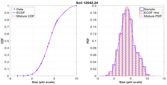
Figure A1.
Soil 12042,24 (“Apollo 12”).
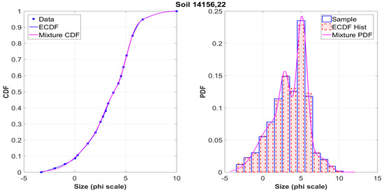
Figure A2.
Soil 14156,22 (“Apollo 14”).
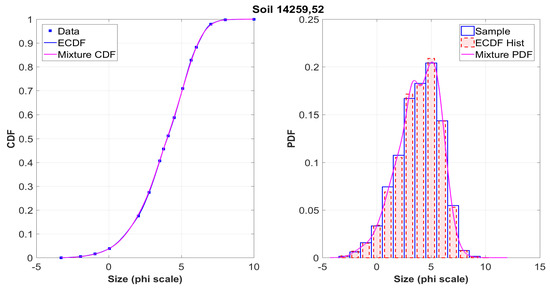
Figure A3.
Soil 14259,52 (“Apollo 14”).
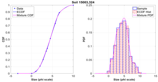
Figure A4.
Soil 15003,324 (“Apollo 15”).
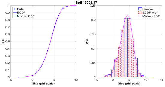
Figure A5.
Soil 15004,17 (“Apollo 15”).
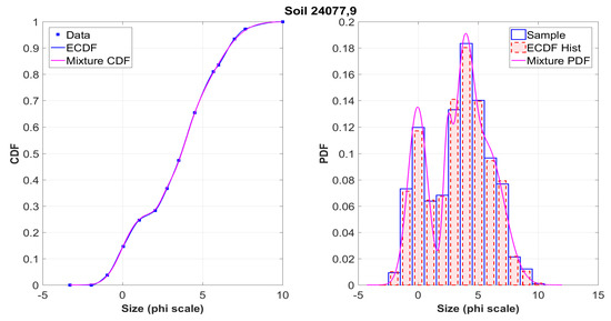
Figure A6.
Soil 24077,9 (“Luna 24”).
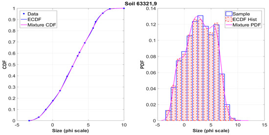
Figure A7.
Soil 63321,9 (“Apollo 16”).
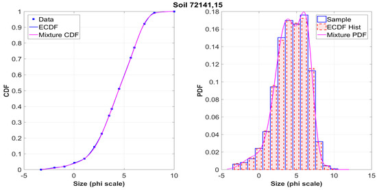
Figure A8.
Soil 72141,15 (“Apollo 17”).
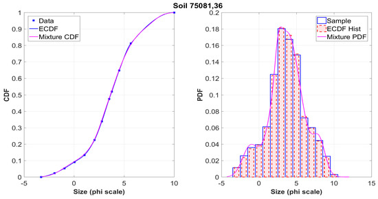
Figure A9.
Soil 75081,36 (“Apollo 17”).
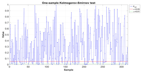
Figure A10.
Approximation errors (one sample Kolmogorov–Smirnov test).
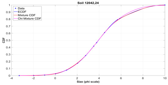
Figure A11.
Soil 12042,24 (“Apollo 12”).
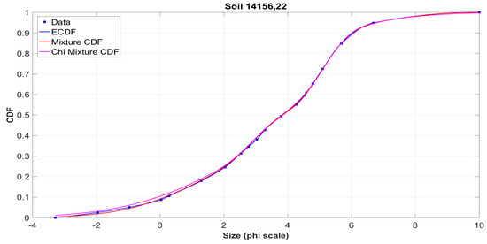
Figure A12.
Soil 14156,22 (“Apollo 14”).
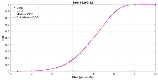
Figure A13.
Soil 14259,52 (“Apollo 14”).
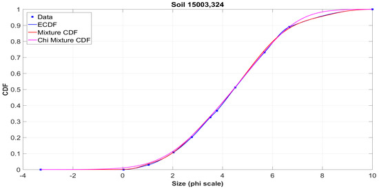
Figure A14.
Soil 15003,324 (“Apollo 15”).
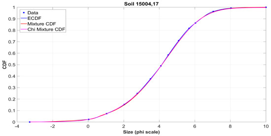
Figure A15.
Soil 15004,17 (“Apollo 15”).
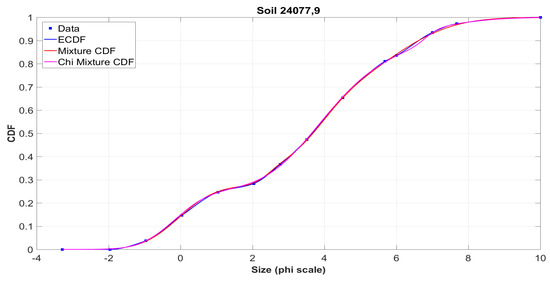
Figure A16.
Soil 24077,9 (“Luna 24”).
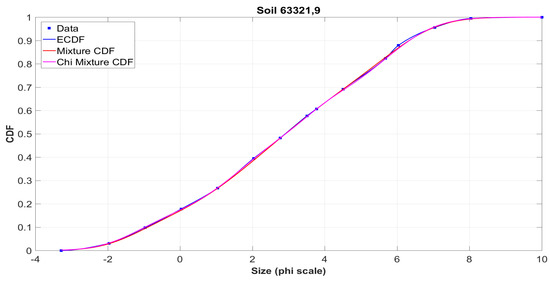
Figure A17.
Soil 63321,9 (“Apollo 16”).
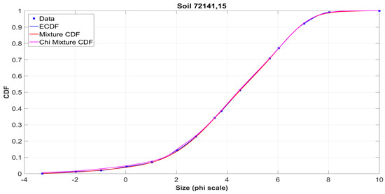
Figure A18.
Soil 72141,15 (“Apollo 17”).
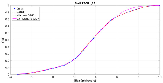
Figure A19.
Soil 75081,36 (“Apollo 17”).
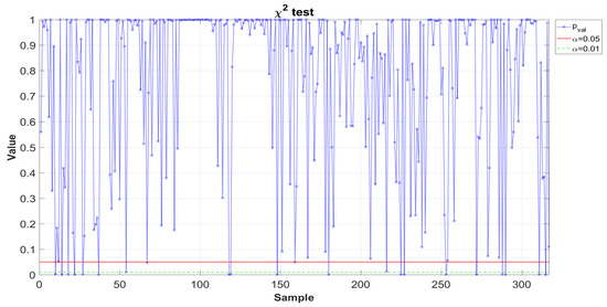
Figure A20.
Approximation errors ( test).
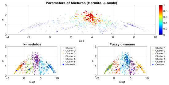
Figure A21.
Clustering the mixture parameters (bootstrap, scale).
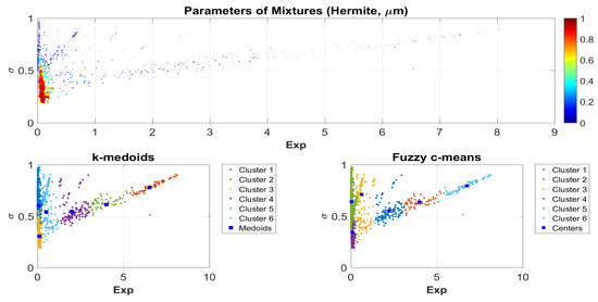
Figure A22.
Clustering the mixture parameters (bootstrap, m).
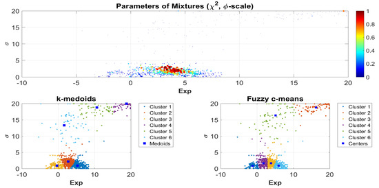
Figure A23.
Clustering the mixture parameters (minimizing estimates, scale).
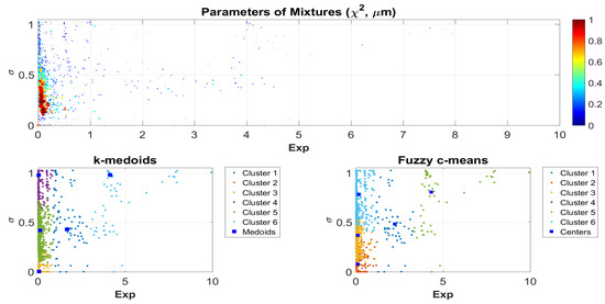
Figure A24.
Clustering the mixture parameters (minimizing estimates, m).
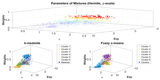
Figure A25.
Clustering the mixture parameters (bootstrap, scale), 3D.
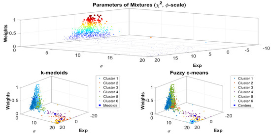
Figure A26.
Clustering the mixture parameters (minimizing estimates, scale), 3D.
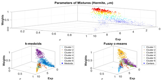
Figure A27.
Clustering the mixture parameters (bootstrap, m), 3D.
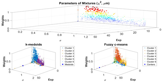
Figure A28.
Clustering the mixture parameters (minimizing estimates, m), 3D.
References
- Popel, S.I.; Zakharov, A.V.; Zelenyi, L.M.; Berezhnoy, A.A.; Zubko, E.S.; Iten, M.; Lena, R.; Sposetti, S.; Velikodsky, Y.I.; Tereshchenko, A.A.; et al. Formation of Dusty Plasma Clouds at Meteoroid Impact on the Surface of the Moon. J. Exp. Theor. Phys. Lett. 2018, 108, 356–363. [Google Scholar] [CrossRef]
- Florenskii, K.P. Lunar Soil: Properties and Analogues; Nauka: Moscow, Russia, 1975. [Google Scholar]
- Korolev, V.Y. On the distribution of particle size under fracturing. Informatics Its Appl. 2009, 3, 60–68. [Google Scholar]
- Korolev, V.Y.; Zeifman, A.I. On convergence of the distributions of random sequences with independent random indexes to variance–mean mixtures. Stoch. Model. 2016, 32, 414–432. [Google Scholar] [CrossRef][Green Version]
- Razumovskii, N.K. The nature of the distribution of metal content in ore deposits. Doklady Akademii Nauk SSSR 1940, 28, 815–817. [Google Scholar]
- Kolmogorov, A.N. On the log-normal law of particle size distribution during fracturing. Doklady Akademii Nauk SSSR 1941, 31, 99–101. [Google Scholar]
- Razumovskii, N.K. Logarithmically normal distribution of matter and its properties. Zapiski Leningradskogo Gornogo Instituta 1948, 20, 105–118. [Google Scholar]
- Bagnold, R.A. The Physics of Blown Sand and Desert Dunes; Methuen: London, UK, 1954. [Google Scholar]
- Reed, W.J.; Jorgensen, M. The double Pareto-Lognormal distribution–a new parametric model for size distribution. Commun. Stat. Theory Methods 2004, 33, 1733–1753. [Google Scholar] [CrossRef]
- Sørensen, M. On the Size Distribution of Sand; Dept. of Applied Mathematics and Statistics, University of Copenhagen: Copenhagen, Denmark, 2006. [Google Scholar]
- Barndorff-Nielsen, O.E. Exponentially decreasing distributions for the logarithm of particle size. Proc. R. Soc. Lond. A Math. Phys. Sci. 1977, 353, 401–419. [Google Scholar] [CrossRef]
- Vincent, P. Differentiation of modern beach and coastal dune sands–a logistic regression approach using the parameters of the hyperbolic function. Sediment. Geol. 1986, 49, 167–176. [Google Scholar] [CrossRef]
- McArthur, D.S. Distinctions between grain-size distribution of accretion and encroachment deposits in an inland dune. Sediment. Geol. 1987, 54, 147–163. [Google Scholar] [CrossRef]
- Hartmann, D. Cross-shore selective sorting process and grain size distributional shape. In Aeolian Grain Transport; Springer: Vienna, Austria, 1991; Volume 2, pp. 49–63. [Google Scholar] [CrossRef]
- Gnedenko, B.V.; Korolev, V.Y. Random Summation: Limit Theorems and Applications; CRC Press: Boca Raton, FL, USA, 1996. [Google Scholar]
- Graf, J.C. Lunar Soils Grain Size Catalog. NASA Ref. Publ. 1993, 1265, 1–508. [Google Scholar]
- Donoghue, J. Encyclopedia of Estuaries (Part of Encyclopedia of Earth Sciences Series); Springer: Dordrecht, The Netherlands, 2016. [Google Scholar] [CrossRef]
- Korolev, V. Convergence of random sequences with independent random indexes. I. Theory Probab. Its Appl. 1994, 39, 313–333. [Google Scholar] [CrossRef]
- Korolev, V. Convergence of random sequences with independent random indexes. II. Theory Probab. Appl. 1995, 40, 770–772. [Google Scholar] [CrossRef]
- Loéve, M. Probability Theory, 3rd ed.; Springer: New York, NY, USA, 1977. [Google Scholar]
- Zolotarev, V. Modern Theory of Summation of Random Variables; VSP: Utrecht, The Netherlands, 1997. [Google Scholar]
- Toda, A.A. Weak limit of the geometric sum of independent but not identically distributed random variables. arXiv 2011, arXiv:1111.1786. [Google Scholar]
- Kubacki, K.S.; Szynal, D. The Convergence of Moments In a Random Limit Theorem of H. Robbins Type. Theory Probab. Appl. 1988, 33, 75–85. [Google Scholar] [CrossRef]
- Kruglov, V.M.; Bo, Z. Weak Convergence of Random Sums. Theory Probab. Appl. 2002, 46, 39–57. [Google Scholar] [CrossRef]
- Teicher, H. Identifiability of finite mixtures. Ann. Math. Stat. 1963, 34, 1265–1269. [Google Scholar] [CrossRef]
- Stineman, R.W. A Consistently Well Behaved Method of Interpolation. Creat. Comput. 1980, 6, 54–57. [Google Scholar]
- Fritsch, F.N.; Carlson, R.E. Monotone Piecewise Cubic Interpolation. SIAM J. Numer. Anal. 1980, 17, 238–246. [Google Scholar] [CrossRef]
- Korolev, V.Y. Probabilistic and Statistical Methods of Decomposition of Volatility of Chaotic Processes; Moscow University Publishing House: Moscow, Russia, 2011. [Google Scholar]
- Waltz, R.A.; Morales, J.L.; Nocedal, J.; Orban, D. An interior algorithm for nonlinear optimization that combines line search and trust region steps. Math. Program. 2006, 107, 391–408. [Google Scholar] [CrossRef]
- Slyuta, E.N. Physical and Mechanical Properties of the Lunar Soil (A Review). Sol. Syst. Res. 2014, 48, 330–353. [Google Scholar] [CrossRef]
© 2020 by the authors. Licensee MDPI, Basel, Switzerland. This article is an open access article distributed under the terms and conditions of the Creative Commons Attribution (CC BY) license (http://creativecommons.org/licenses/by/4.0/).