Strong, Strongly Universal and Weak Interval Eigenvectors in Max-Plus Algebra

Abstract

The optimization problems, such as scheduling or project management, in which the objective function depends on the operations maximum and plus, can be naturally formulated and solved in max-plus algebra. A system of discrete events, e.g., activations of processors in parallel computing, or activations of some other cooperating machines, is described by a systems of max-plus linear equations. In particular, if the system is in a steady state, such as a synchronized computer network in data processing, then the state vector is an eigenvector of the system. In reality, the entries of matrices and vectors are considered as intervals. The properties and recognition algorithms for several types of interval eigenvectors are studied in this paper. For a given interval matrix and interval vector, a set of generators is defined. Then, the strong and the strongly universal eigenvectors are studied and described as max-plus linear combinations of generators. Moreover, a polynomial recognition algorithm is suggested and its correctness is proved. Similar results are presented for the weak eigenvectors. The results are illustrated by numerical examples. The results have a general character and can be applied in every max-plus algebra and every instance of the interval eigenproblem.

1. Introduction

In many practical problems, the standard algebraic operations “plus” and “product” are inadequate, e.g., in scheduling problems, synchronization problems, or in project management, and binary operations “maximum” and “plus” seem to be more appropriate. This observation leads to the definition and use of so-called max-plus algebra, which has been used by many authors, see e.g., [1,2,3,4].

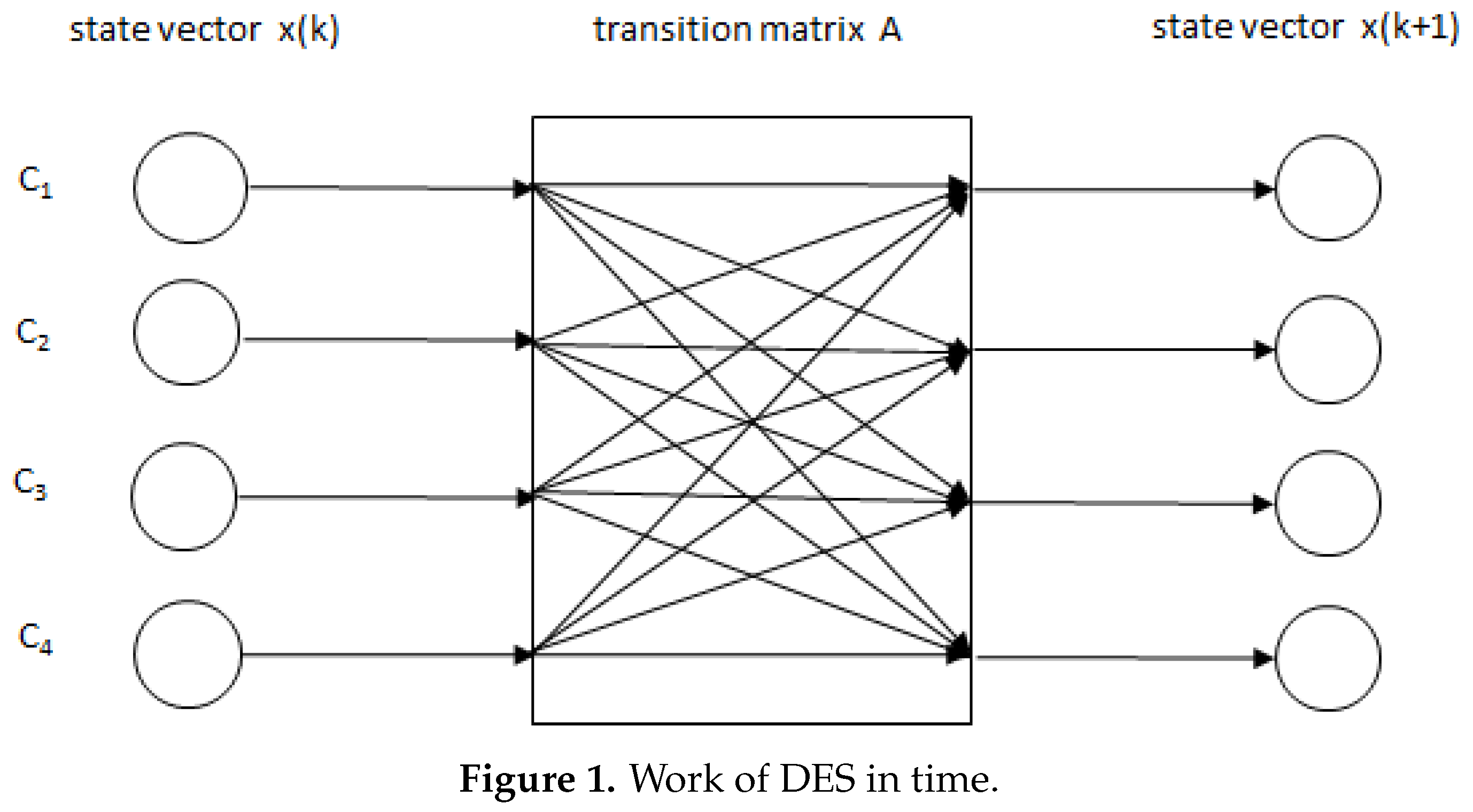
Max-plus algebras represent a suitable mathematical tool for exploration of systems working in discrete steps called discrete event systems (DES, for short). A DES is determined by the transition matrix, A, and the starting state vector, $x^{\left(0\right)}$. The sequence of state vectors in time is then computed by recurrent formula $x^{(k+1)}=A\otimes x^{\left(k\right)}$ using the matrix operations derived from “maximum” and “plus” (for more details, see [2,5,6]).

For convenience of the reader, we present here the basic definitions. A max-plus algebra is a triple $(\mathcal{B},\oplus ,\otimes )$, where $\mathcal{B}$ is the set of real numbers with added $-\infty =\epsilon$, and $\oplus =max$, $\otimes =+$ are binary operations on $\mathcal{B}$. Clearly, $\epsilon$ is the neutral element with respect to ⊕ and the absorbing element with respect to ⊗. $\mathcal{B}(m,n)$ ($\mathcal{B}\left(n\right)$) denote the set of all matrices (vectors) of the given dimension over $\mathcal{B}$. The linear ordering on $\mathcal{B}$ induces a partial ordering on $\mathcal{B}(m,n)$ and $\mathcal{B}\left(n\right)$, with respect to all entries of the matrix (vector).

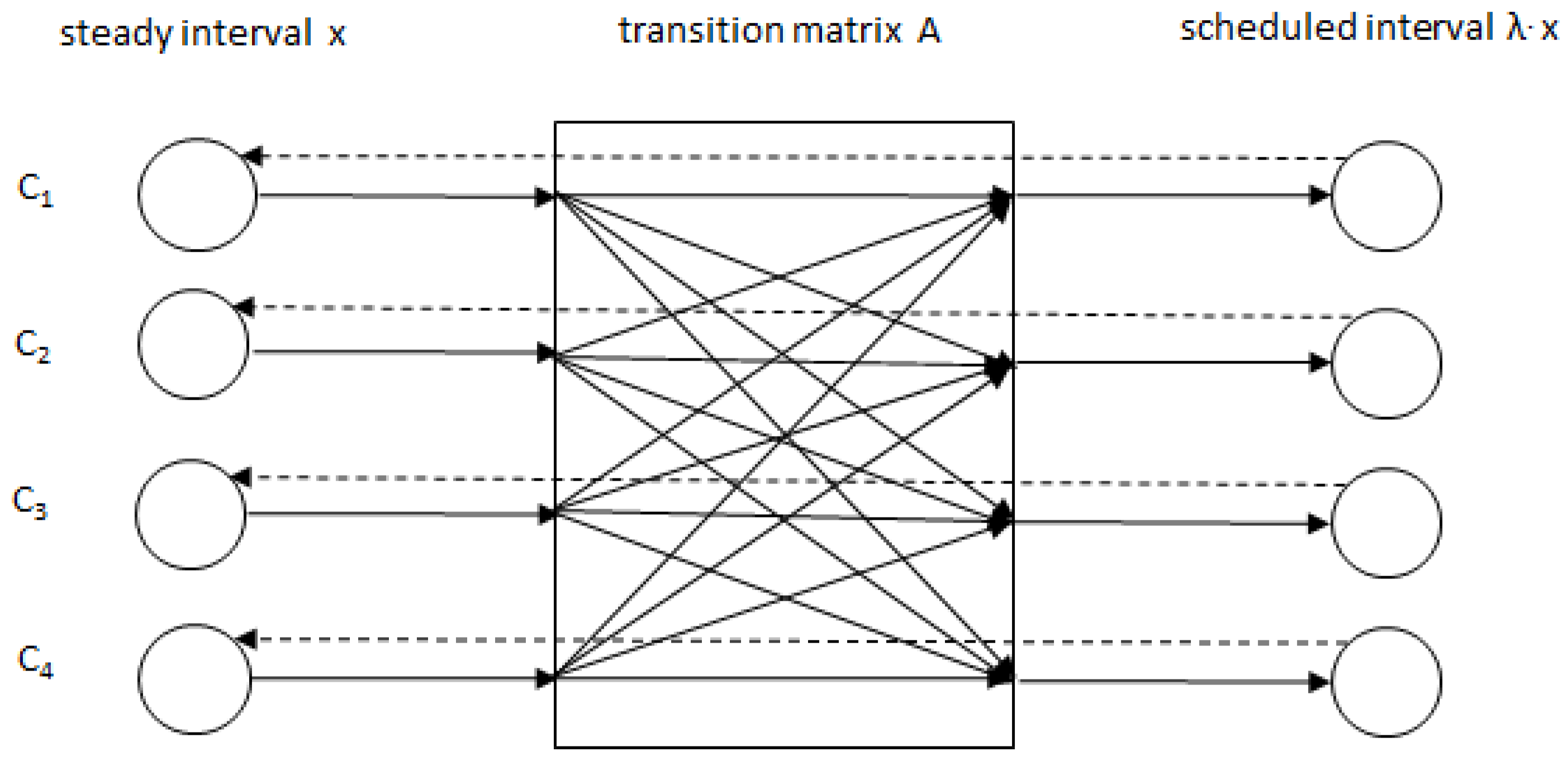
The work of a DES in time often comes to a steady state. In the formal matrix notation, the steady states correspond to max-plus eigenvectors fulfilling the equation $A\otimes x=\lambda \otimes x$, with $A\in \mathcal{B}(n,n)$, $x\in \mathcal{B}\left(n\right)$.

It is assumed that an eigenvector is different from the ‘zero’ vector with all entries equal to $\epsilon$. In this notation, the intervals between the beginnings of consecutive cycles on every component of DES are equal to a scheduled value $\lambda \in \mathcal{B}$.

In the real world, the entries of matrices and vectors are usually not strict values and should be considered as intervals. The properties and recognition algorithms for several types of interval eigenvectors are studied in this paper. The strong, strongly universal and weak interval eigenvectors in max-plus algebra are investigated, and polynomial algorithms for the recognition versions of these problems are presented.

The results can be applied in every max-plus algebra and every instance of the interval eigenproblem.

2. Definitions and Basic Properties

Our results will be illustrated by the following simple example describing the main ideas of the investigation, see Figure 1.

Example 1.

An interactive system consisting of n entities (computers, or some other cooperating machines) working in stages can be represented by discrete-event systems. Denote $C_1,\dots ,C_4$ the computers in parallel computation sharing partial data to continue the computation in the next stage. Suppose $x_i\left(k\right)$ stands for the activation time of the k-th stage on $C_i$$(i=1,\dots ,4)$. Furthermore, suppose that the entries of a matrix A (called the transition matrix) $a_{ij}$ denote the computation time of computer $C_j$ while preparing the data for the work of computer $C_i$ in the $(k+1)$-st stage $(i,j=1,\dots ,4)$. The interference of the system can be described by recurrence relations

$$x_i(k+1)=max\left(x_1\left(k\right)+a_{i1},x_2\left(k\right)+a_{i2},x_3\left(k\right)+a_{i3},x_4\left(k\right)+a_{i4})\right),i\in \{1,2,3,4\}.$$

The considered system can be written in matrix/vector form as $x(k+1)=A\otimes x\left(k\right).$ Moreover, if we schedule for λ the intervals between the beginnings of consecutive cycles on every computer, then we obtain $x(k+1)=\lambda \otimes x\left(k\right)$. Finally, for steady scheduling of the system, we have to solve the equation

$$A\otimes x=\lambda \otimes x.$$

Suppose that the transition matrix A has the form

$$A=\left(\begin{array}{cccc}3& 0& 2& 1\\ 1& 3& 0& 2\\ 2& 1& 3& 0\\ 0& 2& 1& 3\end{array}\right)$$

Then, for the system $A\otimes x=\lambda \otimes x$, we get

$$\left(\begin{array}{cccc}3& 0& 2& 1\\ 1& 3& 0& 2\\ 2& 1& 3& 0\\ 0& 2& 1& 3\end{array}\right)\otimes \left(\begin{array}{c}{x}_1\\ x_2\\ x_3\\ x_4\end{array}\right)=\lambda \otimes \left(\begin{array}{c}{x}_1\\ x_2\\ x_3\\ x_4\end{array}\right)$$

the solution $x={(1,1,1,1)}^T$ which describes the activation times of $C_1,C_2,C_3,C_4$, and the interval between the beginnings of consecutive cycles on every computer is equal to $\lambda =3$. For the work of a steady scheduled DES, see Figure 2.

Remark 1.

In Example 1, the entries $x_i$ are interpreted as activation times of cooperating machines $C_i$ in a DES, while λ is the length of the interval between the beginnings of consecutive cycles in the steady run of the system. This interpretation implies that x cannot contain ε entries. Moreover, by a suitable start of the time-measuring, we can achieve $x_i\ge 0$. The above interpretation gives $\lambda >0$ as well.

Remark 2.

On the other hand, the entries $a_{ij}=\epsilon$ can occur in the transition matrix. The interpretation of such situation is: “$C_i$ need not wait for $C_j$”. Hence, the case $\overline{F}=\{(i,j)\in N;a_{ij}=\epsilon \}=N\times N$ is trivial and is not allowed.

Remark 3.

In LP computations, the constraints with a single ε value on the lower side of the inequality sign are automatically satisfied and may be left out of consideration.

Let us define, similarly as in [7,8,9,10], the interval matrix with bounds $\underline{A},\overline{A}\in \mathcal{B}(n,n)$ and interval vector with bounds $\underline{x},\overline{x}\in \mathcal{B}\left(n\right)$,

$$[\underline{A},\overline{A}]=\left\{A\in \mathcal{B}(n,n);\underline{A}\le A\le \overline{A}\right\},[\underline{x},\overline{x}]=\left\{x\in \mathcal{B}\left(n\right);\underline{x}\le x\le \overline{x}\right\}$$

and suppose that a fixed interval matrix $\mathbf{A}=[\underline{A},\overline{A}]$ and interval vector $\mathbf{X}=[\underline{x},\overline{x}]$ are given. The interval eigenproblem for $\mathbf{A}$ and $\mathbf{X}$ consists of recognizing whether $A\otimes x=\lambda \otimes x$ holds true for $A\in \mathbf{A},x\in \mathbf{X},\lambda \in \mathcal{B}$, with suitable quantifiers (e.g., for all $A\in \mathbf{A}$, for some $A\in \mathbf{A}$, for all $x\in \mathbf{X}$, for some $x\in \mathbf{X}$) and their various combinations. According to the choice of quantifiers and their order, several different types of interval eigenvectors can be defined (see, e.g., [11,12,13] for similar classification). The following three types are studied in detail in this paper.

Definition 1.

Suppose there is a given interval matrix $\mathbf{A}$ and an interval vector $\mathbf{X}$. Then, $\mathbf{X}$ is called

• a strong eigenvector of $\mathbf{A}$
  if $(\exists \lambda \in \mathcal{B})(\forall A\in \mathbf{A})(\forall x\in \mathbf{X})[A\otimes x=\lambda \otimes x]$;
• a strongly universal eigenvector of $\mathbf{A}$
  if $(\exists x\in \mathbf{X})(\exists \lambda \in \mathcal{B})(\forall A\in \mathbf{A})[A\otimes x=\lambda \otimes x]$;
• a weak eigenvector of $\mathbf{A}$
  if $(\exists \lambda \in \mathcal{B})(\exists x\in \mathbf{X})(\exists A\in \mathbf{A})[A\otimes x=\lambda \otimes x]$.

Analogously as the above mentioned interval eigenvectors, the corresponding eigenvalues (the strong eigenvalue, the strongly universal eigenvalue, and the weak eigenvalue) of the interval matrix $\mathbf{A}$ are also defined.

Remark 4.

The investigated ‘universal’ type can be interpreted as follows. In general, the interval vector $\mathbf{X}$ is a universal eigenvector of $\mathbf{A}$ if there is an eigenvalue $\lambda \in \mathcal{B}$ and a vector $x\in \mathbf{X}$, which is a steady state of the discrete event system for every transition matrix $A\in \mathbf{A}$ (in other words, x is a universal eigenvector of $\mathbf{A}$, with eigenvalue λ).

It is welcome in scheduling, when there is one common universal eigenvector $x\in \mathbf{X}$ for all transition matrices $A\in \mathbf{A}$ (the interval vector $\mathbf{X}$ is then called strongly universal). In such situations, it is possible to choose the activation vector within the given interval $[\underline{x},\overline{x}]$, while every possible transition matrix in the given interval is acceptable.

Otherwise, the universal eigenvector x depends on A. If the eigenvalue λ also depends on A, then the interval eigenvector $\mathbf{X}$ is called weakly universal. The universal and weakly universal interval eigenvectors are not studied in this paper.

Remark 5.

A strongly universal eigenvector $x\in \mathbf{X}$ is related to some eigenvalue $\lambda \in \mathcal{B}$, which is independent from A. It is also possible to define a weaker type of interval eigenvector (let us call it: semi-strongly universal) using the formula $(\exists x\in \mathbf{X})(\forall A\in \mathbf{A})(\exists \lambda \in \mathcal{B})[A\otimes x=\lambda \otimes x]$. In this formula, λ depends on A. However, as we prove below in this section, both notions (the strongly universal and the semi-strongly universal) are equivalent.

In the rest of this paper, we use notation $N=\{1,2,\cdots ,n\}$ and assume that an interval matrix $\mathbf{A}=[\underline{A},\overline{A}]$ and an interval vector $\mathbf{X}=[\underline{x},\overline{x}]$ are given.

The following notions of matrix and vector generators are useful. For each pair of indices $i,j\in N$, we define ${\tilde{A}}^{\left(ij\right)}\in \mathcal{B}(n,n)$ and ${\tilde{x}}^{\left(i\right)}\in \mathcal{B}\left(n\right)$ by putting for every $k,l\in N$

$${\tilde{a}}_{kl}^{\left(ij\right)}=\left\{\begin{array}{cc}{\overline{a}}_{ij},\hfill & \mathrm{for}k=i,l=j\hfill \\ {\underline{a}}_{kl},\hfill & \mathrm{otherwise}\hfill \end{array}\right.,{\tilde{x}}_k^{\left(i\right)}=\left\{\begin{array}{cc}{\overline{x}}_i,\hfill & \mathrm{for}k=i\hfill \\ {\underline{x}}_k,\hfill & \mathrm{otherwise}\hfill \end{array}\right..$$

The next lemma says that every matrix in $\mathbf{A}$ can be written as a max-plus linear combination of generating matrices (“generators,” for short) ${\tilde{A}}^{\left(ij\right)}$ with $i,j\in N$. Similarly, every vector in $\mathbf{X}$ is equal to a max-plus linear combination of generators ${\tilde{x}}^{\left(i\right)}$ with $i\in N$.

Lemma 1.

[11] Let $x\in \mathcal{B}\left(n\right)$ and $A\in \mathcal{B}(n,n)$. Then,

(i)

$x\in \mathbf{X}$ if and only if $x={\displaystyle \underset{i\in N}{⨁}}{\beta }_i\otimes {\tilde{x}}^{\left(i\right)}$ for some ${\beta }_i\in \mathcal{B}$ with ${\underline{x}}_i-{\overline{x}}_i\le {\beta }_i\le 0$,

(ii)

$A\in \mathbf{A}$ if and only if $A={\displaystyle \underset{i,j\in N}{⨁}}{\alpha }_{ij}\otimes {\tilde{A}}^{\left(ij\right)}$ for some ${\alpha }_{ij}\in \mathcal{B}$ with ${\underline{a}}_{ij}-{\overline{a}}_{ij}\le {\alpha }_{ij}\le 0$.

Proposition 1.

The interval vector $\mathbf{X}=[\underline{x},\overline{x}]$ is a semi-strongly universal eigenvector of the interval matrix $\mathbf{A}=[\underline{A},\overline{A}]$ if and only if there are $x\in \mathbf{X}$ and ${\lambda }_{ij}\in \mathcal{B},i,j\in N$ such that for every $i,j,k\in N$

$$\begin{array}{cc}\hfill {\tilde{A}}^{\left(ij\right)}\otimes x& ={\lambda }_{ij}\otimes x\hfill \end{array}$$

(1)

$$\begin{array}{cc}\hfill \underset{l\in N}{max}\left({\tilde{a}}_{kl}^{\left(ij\right)}+x_l-x_k\right)& ={\lambda }_{ij}.\hfill \end{array}$$

(2)

Proof. 

Assume $x\in \mathbf{X}$ and ${\lambda }_{ij}\in \mathcal{B},i,j\in N$ fulfill (1). Take any $A\in \mathbf{A}$. Then, by Lemma 1(ii), there are ${\alpha }_{ij}\in \mathcal{B}$ with ${\underline{a}}_{ij}-{\overline{a}}_{ij}\le {\alpha }_{ij}\le 0$, for every $i,j\in N$, such that $A={⨁}_{i,j\in N}{\alpha }_{ij}\otimes {\tilde{A}}^{\left(ij\right)}$. We get

$$\begin{array}{cc}\hfill A\otimes x& =\underset{i,j\in N}{⨁}\left({\alpha }_{ij}\otimes {\tilde{A}}^{\left(ij\right)}\right)\otimes x=\underset{i,j\in N}{⨁}\left({\alpha }_{ij}\otimes {\tilde{A}}^{\left(ij\right)}\otimes x\right)\hfill \end{array}$$

(3)

$$\begin{array}{cc}\hfill & =\underset{i,j\in N}{⨁}\left({\alpha }_{ij}\otimes \left({\lambda }_{ij}\otimes x\right)\right)=\underset{i,j\in N}{⨁}\left({\alpha }_{ij}\otimes {\lambda }_{ij}\right)\otimes x\hfill \end{array}$$

(4)

Write ${\lambda }^A={⨁}_{i,j\in N}\left({\alpha }_{ij}\otimes {\lambda }_{ij}\right)$. Then, (3) and (4) imply $A\otimes x={\lambda }^A\otimes x$. This means that $\mathbf{X}$ is semi-strongly universal, in view of the fact that A was an arbitrary matrix in $\mathbf{A}$. The converse implication is trivial. The equivalence of (1) and (2) follows by easy computation. □

Proposition 2.

The interval vector $\mathbf{X}=[\underline{x},\overline{x}]$ is a semi-strongly universal eigenvector of the interval matrix $\mathbf{A}=[\underline{A},\overline{A}]$ if and only if $\mathbf{X}$ is a strongly universal eigenvector of $\mathbf{A}$.

Proof. 

As a direct consequence of the definition, strong universality implies semi-strong universality with ${\lambda }_{ij}=\lambda$ for all $i,j\in N$.

To show the converse implication, let us assume that $\mathbf{X}$ is a semi-strongly universal eigenvector of $\mathbf{A}$. Then, in view of (2), there are $x\in \mathbf{X}$ and ${\lambda }_{ij}\in \mathcal{B},i,j\in N$ such that

$$\begin{array}{cc}\hfill \underset{l\in N}{max}\left({\tilde{a}}_{kl}^{\left(ij\right)}+x_l-x_k\right)& ={\lambda }_{ij}\mathrm{for} \mathrm{every} i,j,k\in N.\hfill \end{array}$$

(5)

For fixed $i,j,k\in N$, (5) is equivalent to

$$\begin{array}{cc}\hfill {\tilde{a}}_{kl}^{\left(ij\right)}+x_l-x_k& \le {\lambda }_{ij}\mathrm{for} \mathrm{every} l\in N,\hfill \end{array}$$

(6)

$$\begin{array}{cc}\hfill {\tilde{a}}_{kl}^{\left(ij\right)}+x_l-x_k& ={\lambda }_{ij}\mathrm{for} \mathrm{every} l\in N.\hfill \end{array}$$

(7)

Claim 1. $\left(\forall i,j\in N\right)\left(\exists (k,l)\ne (i,j)\right)\left[{\underline{a}}_{kl}+x_l-x_k={\lambda }_{ij}\right].$

Proof of Claim 1. Let $i,j\in N$ be fixed. Take $k\in N\backslash \left\{i\right\}$. Then, by (7), there is $l\in N$ such that

$${\underline{a}}_{kl}+x_l-x_k={\tilde{a}}_{kl}^{\left(ij\right)}+x_l-x_k={\lambda }_{ij}.$$

Claim 2. $\left(\forall i,j,h,g\in N\right)\left[{\lambda }_{ij}={\lambda }_{hg}\right].$

Proof of Claim 2. Let $i,j\in N$ be fixed. In view of Claim 1 and inequality (6), for every $k\in N$, there is $l\in N$ such that

$${\lambda }_{ij}={\underline{a}}_{kl}+x_l-x_k\le {\tilde{a}}_{kl}^{\left(hg\right)}+x_l-x_k\le {\lambda }_{hg}.$$

We have shown that ${\lambda }_{ij}\le {\lambda }_{hg}.$ As $i,j,h,g\in N$ were arbitrary, ${\lambda }_{ij}={\lambda }_{hg}$ follows. By this, the proof of the proposition is complete. □

3. Strong Interval Eigenvectors in a Max-Plus Algebra

When the interval entries in the interval eigenproblem are narrow, then the scheduling is possible by any activation vector and any transition matrix in the given limits. A necessary and sufficient condition for recognizing this situation is described in this section.

Proposition 3.

The interval vector $\mathbf{X}=[\underline{x},\overline{x}]$ is a strong eigenvector of the interval matrix $\mathbf{A}=[\underline{A},\overline{A}]$ if and only if there is $\lambda \in \mathcal{B}$ such that for every $i\in N$

$$\begin{array}{cc}\hfill \underline{A}\otimes {\tilde{x}}^{\left(i\right)}& =\lambda \otimes {\tilde{x}}^{\left(i\right)},\hfill \end{array}$$

(8)

$$\begin{array}{cc}\hfill \overline{A}\otimes {\tilde{x}}^{\left(i\right)}& =\lambda \otimes {\tilde{x}}^{\left(i\right)}.\hfill \end{array}$$

(9)

Proof. 

Assume $\lambda \in \mathcal{B}$ and ${\tilde{x}}^{\left(i\right)}\in \mathbf{X}$ with $i\in N$ fulfill (8) and (9). Take any $A\in \mathbf{A}$, that is, $\underline{A}\le A\le \overline{A}$. Then, $\underline{A}\otimes {\tilde{x}}^{\left(i\right)}\le A\otimes {\tilde{x}}^{\left(i\right)}\le \overline{A}\otimes {\tilde{x}}^{\left(i\right)}$ by the monotonicity of the operations in a max-plus algebra. This implies $A\otimes {\tilde{x}}^{\left(i\right)}=\lambda \otimes {\tilde{x}}^{\left(i\right)}$, in view of (8) and (9).

By Lemma 1(i), every $x\in \mathbf{X}$ can be written as $x={⨁}_{i\in N}{\beta }_i\otimes {\tilde{x}}^{\left(i\right)}$ for some ${\beta }_i\in \mathcal{B}$ with ${\underline{x}}_i-{\overline{x}}_i\le {\beta }_i\le 0$. Then,

$$\begin{array}{ccc}\hfill A\otimes x& =A\otimes \left(\underset{i\in N}{⨁}{\beta }_i\otimes {\tilde{x}}^{\left(i\right)}\right)=\left(\underset{i\in N}{⨁}A\otimes \left({\beta }_i\otimes {\tilde{x}}^{\left(i\right)}\right)\right)\hfill & \hfill \left(10\right)\\ \hfill & =\left(\underset{i\in N}{⨁}{\beta }_i\otimes \left(A\otimes {\tilde{x}}^{\left(i\right)}\right)\right)=\left(\underset{i\in N}{⨁}{\beta }_i\otimes \left(\lambda \otimes {\tilde{x}}^{\left(i\right)}\right)\right)\hfill & \hfill \left(11\right)\\ \hfill & =\left(\underset{i\in N}{⨁}\lambda \otimes \left({\beta }_i\otimes {\tilde{x}}^{\left(i\right)}\right)\right)=\lambda \otimes \left(\underset{i\in N}{⨁}\left({\beta }_i\otimes {\tilde{x}}^{\left(i\right)}\right)\right)=\lambda \otimes x.\hfill & \hfill \left(12\right)\end{array}$$

The converse implication is trivial. □

Remark 6.

The eigenvalue λ of a strong interval eigenvector is uniquely determined by the entries of the $2n$ vectors with $i\in N$

$$\begin{array}{cc}\hfill \underline{A}\otimes {\tilde{x}}^{\left(i\right)}-{\tilde{x}}^{\left(i\right)}& ={(\lambda ,\lambda ,\dots \lambda )}^T,\hfill \end{array}$$

(13)

$$\begin{array}{cc}\hfill \overline{A}\otimes {\tilde{x}}^{\left(i\right)}-{\tilde{x}}^{\left(i\right)}& ={(\lambda ,\lambda ,\dots \lambda )}^T.\hfill \end{array}$$

(14)

These deciding values are computed from the entries of $\underline{A},\overline{A},\underline{x},$ and $\overline{x}$. If the computed values are equal, then their common value λ is the unique eigenvalue of the problem, and the given interval vector $\mathbf{X}$ is a strong eigenvector of $\mathbf{A}$. Otherwise, the interval eigenvector $\mathbf{X}$ is not a strong one.

Corollary 1.

The problem of recognizing whether a given interval vector $\mathbf{X}$ is a strong eigenvector of a given interval matrix $\mathbf{A}$ in max-plus algebra is solvable by computing $2n$ matrix products and by verifying $2n^2$ max-plus linear equalities, hence, in $O\left(n^3\right)$-time.

Example 2.

Assume now that the entries of $\mathbf{X}$ and $\mathbf{A}$ are intervals which contain values with the same importance and all values of the interval must be taken into account, i.e., there is an eigenvalue $\lambda \in \mathcal{B}$ such that, for every vector $x\in \mathbf{X}$ and, for every transition matrix $A\in \mathbf{A}$, the corresponding DES is in steady state. In other words, each $x\in \mathbf{X}$ is an eigenvector of each $A\in \mathbf{A}$ with the same eigenvalue λ.

Suppose that $\mathbf{A}$ and $\mathbf{X}$ are of the form

$$\underline{A}=\left(\begin{array}{cccc}3& 0& 2& 1\\ 1& 3& 0& 2\\ 2& 1& 3& 0\\ 0& 2& 1& 3\end{array}\right),\overline{A}=\left(\begin{array}{cccc}3& 1& 2& 2\\ 2& 3& 1& 2\\ 2& 2& 3& 1\\ 1& 2& 2& 3\end{array}\right)$$

$$\underline{x}=\left(\begin{array}{c}\hfill 0\\ \hfill 0\\ \hfill 0\\ \hfill 0\end{array}\right),\overline{x}=\left(\begin{array}{c}\hfill 1\\ \hfill 1\\ \hfill 1\\ \hfill 1\end{array}\right).$$

The goal is to recognize whether $\mathbf{X}$ is a strong eigenvector of $\mathbf{A}$. By direct computation, we get

$${\tilde{x}}^{\left(1\right)}=\left(\begin{array}{c}\hfill 1\\ \hfill 0\\ \hfill 0\\ \hfill 0\end{array}\right),{\tilde{x}}^{\left(2\right)}=\left(\begin{array}{c}\hfill 0\\ \hfill 1\\ \hfill 0\\ \hfill 0\end{array}\right),{\tilde{x}}^{\left(3\right)}=\left(\begin{array}{c}\hfill 0\\ \hfill 0\\ \hfill 1\\ \hfill 0\end{array}\right),{\tilde{x}}^{\left(4\right)}=\left(\begin{array}{c}\hfill 0\\ \hfill 0\\ \hfill 0\\ \hfill 1\end{array}\right)$$

and

$$\underline{A}\otimes {\tilde{x}}^{\left(1\right)}=\left(\begin{array}{c}\hfill 4\\ \hfill 3\\ \hfill 3\\ \hfill 3\end{array}\right),\underline{A}\otimes {\tilde{x}}^{\left(2\right)}=\left(\begin{array}{c}\hfill 3\\ \hfill 4\\ \hfill 3\\ \hfill 3\end{array}\right),\underline{A}\otimes {\tilde{x}}^{\left(3\right)}=\left(\begin{array}{c}\hfill 3\\ \hfill 3\\ \hfill 4\\ \hfill 3\end{array}\right),\underline{A}\otimes {\tilde{x}}^{\left(4\right)}=\left(\begin{array}{c}\hfill 3\\ \hfill 3\\ \hfill 3\\ \hfill 4\end{array}\right),$$

$$\overline{A}\otimes {\tilde{x}}^{\left(1\right)}=\left(\begin{array}{c}\hfill 4\\ \hfill 3\\ \hfill 3\\ \hfill 3\end{array}\right),\overline{A}\otimes {\tilde{x}}^{\left(2\right)}=\left(\begin{array}{c}\hfill 3\\ \hfill 4\\ \hfill 3\\ \hfill 3\end{array}\right),\overline{A}\otimes {\tilde{x}}^{\left(3\right)}=\left(\begin{array}{c}\hfill 3\\ \hfill 3\\ \hfill 4\\ \hfill 3\end{array}\right),\overline{A}\otimes {\tilde{x}}^{\left(4\right)}=\left(\begin{array}{c}\hfill 3\\ \hfill 3\\ \hfill 3\\ \hfill 4\end{array}\right).$$

After subtracting generators ${\tilde{x}}^{\left(1\right)}$, ${\tilde{x}}^{\left(2\right)}$, ${\tilde{x}}^{\left(3\right)}$, ${\tilde{x}}^{\left(4\right)}$, we get

$$\underline{A}\otimes {\tilde{x}}^{\left(i\right)}-{\tilde{x}}^{\left(i\right)}=\overline{A}\otimes {\tilde{x}}^{\left(i\right)}-{\tilde{x}}^{\left(i\right)}={(3,3,3,3)}^T,$$

for every $i\in \{1,2,3,4\}.$ In view of (13) and (14), we have shown that $\mathbf{X}$ is a strong eigenvector of $\mathbf{A}$ with $\lambda =3$.

4. Strongly Universal Interval Eigenvectors in a Max-Plus Algebra

In a strongly universal case, there is one (so-called: universal) eigenvector $x\in \mathbf{X}$ which corresponds to all transition matrices in the given interval $\mathbf{A}$. Then, the scheduled run of the DES with the starting state x is satisfied in every stage, if the transition matrix is kept within the $\mathbf{A}$ limits.

Proposition 4.

Let $\underline{x},\overline{x}\in \mathcal{B}\left(n\right)$, $\underline{A},\overline{A}\in \mathcal{B}(n,n)$. The interval vector $\mathbf{X}=[\underline{x},\overline{x}]$ is a strongly universal eigenvector of the interval matrix $\mathbf{A}=[\underline{A},\overline{A}]$ if and only if there are $\lambda \in \mathcal{B}$ and $x\in \mathbf{X}$ such that

$$\begin{array}{cc}\hfill \underline{A}\otimes x& =\lambda \otimes x,\hfill \end{array}$$

(15)

$$\begin{array}{cc}\hfill \overline{A}\otimes x& =\lambda \otimes x.\hfill \end{array}$$

(16)

Proof. 

Assume $\lambda \in \mathcal{B}$, and $x\in \mathbf{X}$ fulfill (15) and (16). Take any $A\in \mathbf{A}$, that is, $\underline{A}\le A\le \overline{A}$. Then, $\underline{A}\otimes x\le A\otimes x\le \overline{A}\otimes x$, by the monotonicity of the operations in a max-plus algebra. This implies $A\otimes x=\lambda \otimes x$, in view of (15) and (16). The converse implication is trivial. □

LP approach.

The existence of $\lambda \in \mathcal{B}$, and $x\in \mathbf{X}$ in Proposition 4 satisfying (15) and (16) can be recognized by solving the following linear programming problem: ${\mathcal{P}}_{su}$ with variables $\lambda$, $x_1,x_2,\dots ,x_n$

$$z=\lambda \to min$$

(17)

subject to

$$\begin{array}{cc}\hfill {\overline{a}}_{ij}-x_i+x_j& \le \lambda \mathrm{for} \mathrm{every} i,j\in N,\hfill \end{array}$$

(18)

$$\begin{array}{cc}\hfill {\underline{x}}_j& \le x_j\mathrm{for} \mathrm{every} j\in N,\hfill \end{array}$$

(19)

$$\begin{array}{cc}\hfill x_j& \le {\overline{x}}_j\mathrm{for} \mathrm{every} j\in N.\hfill \end{array}$$

(20)

Theorem 1.

The interval vector $\mathbf{X}=[\underline{x},\overline{x}]$, $\underline{x},\overline{x}\in \mathcal{B}\left(n\right)$, is a strongly universal eigenvector of the interval matrix $\mathbf{A}=[\underline{A},\overline{A}]$, $\underline{A},\overline{A}\in \mathcal{B}(n,n)$, if and only if the minimization problem (17)–(20) has an optimal solution satisfying

$$\begin{array}{cc}\hfill \underset{j\in N}{max}({\underline{a}}_{ij}-x_i+x_j)& =\lambda \mathrm{for} \mathrm{every} i\in N,\hfill \end{array}$$

(21)

$$\begin{array}{cc}\hfill \underset{j\in N}{max}({\overline{a}}_{ij}-x_i+x_j)& =\lambda \mathrm{for} \mathrm{every} i\in N.\hfill \end{array}$$

(22)

Proof. 

It is easy to see that, for every pair $(i,j)\in \overline{F}$, the equality ${\overline{a}}_{ij}=\epsilon$ implies that (18) is automatically satisfied. That is, this constraint has only to be considered for $(i,j)\in N\times N\backslash \overline{F}$ (see Remark 3). Analogous limitations are to be applied in (21) and (22).

Now, let us assume that ${\lambda }^{opt}$ and $x^{opt}$ are optimal solutions of (17)–(20) with (21) and (22). Then, (15) and (16) follow by a simple transformation. In view of Proposition 4, $\mathbf{X}$ is strongly universal.

Conversely, assume that $\mathbf{X}=[\underline{x},\overline{x}]$ is a strongly universal eigenvector of $\mathbf{A}=[\underline{A},\overline{A}]$. Then, by Proposition 4, there are $\lambda \in \mathcal{B}$ and $x\in \mathbf{X}$ satisfying (15) and (16). By easy equivalent modifications, we see that $\lambda$ and x satisfy (21) and (22).

Thus, for every $i\in N$, $\lambda$ is the least upper bound of the set of all $({\underline{a}}_{ij}-x_i+x_j)$ with $j\in N$ (and also the least upper bound of the set of all $({\overline{a}}_{ij}-x_i+x_j)$ with $j\in N$ and $(i,j)\notin \overline{F}$). That is, $\lambda ,x$ is an optimal solution of the minimization problem (17)–(20). □

Corollary 2.

The problem of recognizing whether a given interval vector $\mathbf{X}$ is a strongly universal eigenvector of a given interval matrix $\mathbf{A}$ in a max-plus algebra is solvable with the help of an LP minimization problem with $n+1$ variables and $2n^2+2n$ constraints, and by verifying $2n$ max-plus linear equations in $O\left(n^3\right)$-time.

Proof. 

The assertion follows from Remark 2 and Theorem 1. □

Example 3.

Assume that the entries of $\mathbf{X}$ and $\mathbf{A}$ are intervals and we look for an eigenvalue $\lambda \in \mathcal{B}$ and a vector $x\in \mathbf{X}$ such that, for every transition matrix, $A\in \mathbf{A}$ is the corresponding DES in a steady state.

Suppose that $\mathbf{A}$, $\mathbf{X}$ are of the forms

$$\underline{A}=\left(\begin{array}{cccc}3& 0& 2& 1\\ 1& 0& 0& 2\\ 2& 1& 3& 0\\ 0& 2& 1& 3\end{array}\right),\overline{A}=\left(\begin{array}{cccc}3& 1& 2& 2\\ 2& 1& 1& 2\\ 2& 2& 3& 1\\ 1& 2& 2& 3\end{array}\right)$$

$$\underline{x}=\left(\begin{array}{c}\hfill 0\\ \hfill 0\\ \hfill 0\\ \hfill 0\end{array}\right),\overline{x}=\left(\begin{array}{c}\hfill 2\\ \hfill 1\\ \hfill 2\\ \hfill 3\end{array}\right).$$

The goal is to decide whether $\mathbf{X}$ is a strongly universal eigenvector of $\mathbf{A}$. By solving the minimization problem (17)–(20), we get the optimal solution ${\lambda }^{opt}=3$, $x^{opt}={(2,1,2,2)}^T$ satisfying (21), in Theorem 1. Now, after easy computation, we get

$$\underline{A}\otimes x^{opt}=\left(\begin{array}{cccc}3& 0& 2& 1\\ 1& 0& 0& 2\\ 2& 1& 3& 0\\ 0& 2& 1& 3\end{array}\right)\otimes \left(\begin{array}{c}\hfill 2\\ \hfill 1\\ \hfill 2\\ \hfill 2\end{array}\right)=\left(\begin{array}{c}\hfill 5\\ \hfill 4\\ \hfill 5\\ \hfill 5\end{array}\right)={\lambda }^{opt}\otimes x^{opt}.$$

$$\overline{A}\otimes x^{opt}=\left(\begin{array}{cccc}3& 1& 2& 2\\ 2& 3& 1& 2\\ 2& 2& 3& 1\\ 1& 2& 2& 3\end{array}\right)\otimes \left(\begin{array}{c}2\\ 1\\ 2\\ 2\end{array}\right)=\left(\begin{array}{c}\hfill 5\\ \hfill 4\\ \hfill 5\\ \hfill 5\end{array}\right)={\lambda }^{opt}\otimes x^{opt}.$$

Thus, in view of Proposition 4, $\mathbf{X}$ is a strongly universal eigenvector of $\mathbf{A}$, with scheduled starting state vector $x^{opt}={(2,1,2,2)}^T$ and ${\lambda }^{opt}=3$.

Remark 7.

It is worth mentioning that, on the other hand, $\mathbf{X}$ is not a strong eigenvector of $\mathbf{A}$ because the condition (13) in Remark 6 is not satisfied. In particular, $\underline{A}\otimes {\tilde{x}}^{\left(1\right)}-{\tilde{x}}^{\left(1\right)}={(3,4,4,3)}^T\ne {(3.3.3.3)}^T={({\lambda }^{opt},{\lambda }^{opt},{\lambda }^{opt},{\lambda }^{opt})}^T$. This shows that a stronly universal interval eigenvector need not be a strong interval eigenvector.

Example 4.

In this example, we illustrate the influence of ε entries in the transition matrix on the computation. The interval vector $\mathbf{X}$ is the same as in Example 3. Some of the entries of $\mathbf{A}$ are substituted by $-1000$, playing the the role of $-\infty$, and the rest remains unchanged.

Case A. Consider matrix $\mathbf{A}=[\underline{A},\overline{A}]$ with

$$\underline{A}=\left(\begin{array}{cccc}3& 0& 2& 1\\ 1& 0& 0& 2\\ 2& 1& 3& 0\\ 0& -1000& -1000& 3\end{array}\right),\overline{A}=\left(\begin{array}{cccc}3& 1& 2& 2\\ 2& 1& 1& 2\\ 2& 2& 3& 1\\ 1& 2& 2& 3\end{array}\right)$$

The optimal solution of the minimization problem in this case is ${\lambda }^{opt}=3$, $x^{opt}={(2,1,1,0)}^T$. Similarly as in Example 3, an easy computation gives $\underline{A}\otimes x^{opt}={\lambda }^{opt}\otimes x^{opt}$ and $\overline{A}\otimes x^{opt}={\lambda }^{opt}\otimes x^{opt}.$

Case B.

$$\underline{A}=\left(\begin{array}{cccc}3& 0& 2& 1\\ 1& 3& 0& 2\\ 2& 1& 3& 0\\ -1000& 2& 1& 3\end{array}\right),\overline{A}=\left(\begin{array}{cccc}3& 1& 2& 2\\ 2& 0& 1& 2\\ 2& 2& 3& 1\\ 1& 2& 2& 3\end{array}\right)$$

The optimal solution of the minimization problem in this case is ${\lambda }^{opt}=3$, $x^{opt}={(0,0,0,0)}^T$.

Case C.

$$\underline{A}=\left(\begin{array}{cccc}3& 0& 2& 1\\ 1& 0& 0& 2\\ 2& 1& 3& 0\\ 0& 2& -1000& 3\end{array}\right),\overline{A}=\left(\begin{array}{cccc}3& 1& 2& 2\\ 2& 1& 1& 2\\ 2& 2& 3& 1\\ 1& 2& 2& 3\end{array}\right)$$

The optimal solution of the minimization problem in this case is ${\lambda }^{opt}=3$, $x^{opt}={(2,1,1,0)}^T$.

5. Weak Interval Eigenvectors in a Max-Plus Algebra

This section uses the general properties of the eigenvalue in interval eigenproblems that have been demonstrated in [11]. Suppose that there is an interval matrix $\mathbf{A}=[\underline{A},\overline{A}]$ and a vector $x\in \mathcal{B}\left(n\right)$. Write

$$\begin{array}{ccc}\hfill \underline{\lambda }\left(x\right)& =& \underset{i\in N}{max}\underset{j\in N}{max}({\underline{a}}_{ij}-x_i+x_j)\hfill \end{array}$$

(23)

$$\begin{array}{ccc}\hfill \overline{\lambda }\left(x\right)& =& \underset{i\in N}{min}\underset{j\in N}{max}({\overline{a}}_{ij}-x_i+x_j).\hfill \end{array}$$

(24)

Lemma 2

([11]). Let $x\in \mathcal{B}\left(n\right)$ and $\lambda \in \mathcal{B}$. Then,

$$(\exists A^{\star }\in \mathbf{A})A^{\star }\otimes x=\lambda \otimes x$$

if and only if

$$\underline{\lambda }\left(x\right)\le \lambda \le \overline{\lambda }\left(x\right).$$

(25)

Proposition 5.

The interval vector $\mathbf{X}=[\underline{x},\overline{x}]$ is a weak eigenvector of the interval matrix $\mathbf{A}=[\underline{A},\overline{A}]$ if and only if there are $\lambda \in \mathcal{B}$ and $x\in \mathbf{X}$ such that

$$\begin{array}{cc}\hfill \underset{i\in N}{max}\underset{j\in N}{max}({\underline{a}}_{ij}-x_i+x_j)& \le \lambda ,\hfill \end{array}$$

(26)

$$\begin{array}{cc}\hfill \lambda & \le \underset{i\in N}{min}\underset{j\in N}{max}({\overline{a}}_{ij}-x_i+x_j).\hfill \end{array}$$

(27)

Proof. 

Assume $\lambda \in \mathcal{B}$ and $x\in \mathbf{X}$ fulfill (26) and (27). Then, (25) follows from (23) and (24). Thus, $\mathbf{X}$ is a weak eigenvector of $\mathbf{A}$ by Lemma 2.

Conversely, if $\mathbf{X}$ is a weak eigenvector of $\mathbf{A}$, then there are $\lambda \in \mathcal{B}$, $x\in \mathbf{X}$, and $A\in \mathbf{A}$ such that $A\otimes x=\lambda \otimes x$. As a consequence, (25) holds, by Lemma 2. In view of (23) and (24), we have (26) and (27). □

Remark 8.

If the conditions (26) and (27) are satisfied for given $\lambda \in \mathcal{B}$ and $x\in \mathbf{X}$, then the matrix $A^{\star }$ with $A^{\star }\otimes x=\lambda \otimes x$ can be constructed by the following procedure, described in [11], Lemma 4.2. In view of the condition

$$\lambda \le \overline{\lambda }\left(x\right)=\underset{i\in N}{min}\underset{j\in N}{max}({\overline{a}}_{ij}-x_i+x_j),$$

there is a $\phi :N\to N$ such that, for every $i\in N$,

$$\lambda \le {\overline{a}}_{i\phi \left(i\right)}-x_i+x_{\phi \left(i\right)}.$$

(28)

Choose a mapping φ fulfilling (28) and then define a matrix $A^{\star }\in \mathcal{B}(n,n)$ by putting

$$a_{ij}^{\star }=\left\{\begin{array}{cc}\lambda +x_i-x_j\hfill & ifj=\phi \left(i\right)\hfill \\ {\underline{a}}_{ij}\hfill & otherwise.\hfill \end{array}\right.$$

(29)

In view of (28) and (29), we have for every $i\in N$

$$a_{i\phi \left(i\right)}^{\star }=\lambda +x_i-x_{\phi \left(i\right)}\le \left({\overline{a}}_{i\phi \left(i\right)}-x_i+x_{\phi \left(i\right)}\right)+x_i-x_{\phi \left(i\right)}={\overline{a}}_{i\phi \left(i\right)}$$

and hence $A^{\star }\le \overline{A}$. On the other hand, the condition

$$\underline{\lambda }\left(x\right)=\underset{i\in N}{max}\underset{j\in N}{max}({\underline{a}}_{ij}-x_i+x_j)\le \lambda$$

implies that, for every $i\in N$,

$${\underline{a}}_{i\phi \left(i\right)}=\left({\underline{a}}_{i\phi \left(i\right)}-x_i+x_{\phi \left(i\right)}\right)+x_i-x_{\phi \left(i\right)}\le \lambda +x_i-x_{\phi \left(i\right)}=a_{i\phi \left(i\right)}^{\star },$$

hence $\underline{A}\le A^{\star }$. That is, $A^{\star }\in \mathbf{A}$. Furthermore, we have, for every $i,j\in N$,

$$\begin{array}{cc}\hfill a_{ij}^{\star }-x_i+x_j=(\lambda +x_i-x_j)-x_i+x_j=\lambda & ifj=\phi \left(i\right)\hfill \end{array}$$

(30)

$$\begin{array}{cc}\hfill a_{ij}^{\star }-x_i+x_j={\underline{a}}_{ij}-x_i+x_j\le \underline{\lambda }\left(x\right)\le \lambda & otherwise.\hfill \end{array}$$

(31)

By an easy modification of (30) and (31), we get $A^{\star }\otimes x=\lambda \otimes x$.

LP approach.

The existence of $\lambda \in \mathcal{B}$ and $x\in \mathbf{X}$ satisfying (26) and (27) can be recognized by solving the following linear programming problem $\mathcal{P}$ with variables $\lambda$, $u_1,u_2,\dots ,u_n$, $x_1,x_2,\dots ,x_n$

$$z=\sum _{i\in N}{u}_i\to min$$

(32)

subject to

$$\begin{array}{cc}\hfill {\underline{a}}_{ij}-x_i+x_j& \le \lambda \mathrm{for} \mathrm{every} i,j\in N,\hfill \end{array}$$

(33)

$$\begin{array}{cc}\hfill \lambda & \le u_i\mathrm{for} \mathrm{every}i\in N,\hfill \end{array}$$

(34)

$$\begin{array}{cc}\hfill {\overline{a}}_{ij}-x_i+x_j& \le u_i\mathrm{for} \mathrm{every}i,j\in N,\hfill \end{array}$$

(35)

$$\begin{array}{cc}\hfill {\underline{x}}_j& \le x_j\mathrm{for} \mathrm{every}j\in N,\hfill \end{array}$$

(36)

$$\begin{array}{cc}\hfill x_j& \le {\overline{x}}_j\mathrm{for} \mathrm{every}j\in N.\hfill \end{array}$$

(37)

Remark 9.

Note that ${\underline{a}}_{ij}-{\overline{x}}_i+{\underline{x}}_j\le {\underline{a}}_{ij}-x_i+x_j\le \lambda \le u_i$ for every $i,j\in N$. That is, the objective function $z={\sum }_{i\in N}{u}_i$ is bounded from below. As a consequence, if there is a feasible solution of $\mathcal{P}$, then $\mathcal{P}$ has at least one optimal solution.

Theorem 2.

The interval vector $\mathbf{X}=[\underline{x},\overline{x}]$ is a weak eigenvector of the interval matrix $\mathbf{A}=[\underline{A},\overline{A}]$ if and only if the minimization problem (32)–(37) has an optimal solution satisfying

$$\begin{array}{cc}\hfill \underset{j\in N}{max}({\overline{a}}_{ij}-x_i+x_j)& =u_i\mathrm{for} \mathrm{every}i\in N.\hfill \end{array}$$

(38)

Proof. 

Assume that $z^{opt}={\sum }_{i\in N}{u}_i^{opt}$ is the optimal value of the objective function (32) and ${\lambda }^{opt}$, $u_i^{opt}$, $x_j^{opt}$, with $i,j\in N$ satisfying (33)–(38). Then, inequalities (33) imply (26). Similarly, (35) implies ${max}_{j\in N}({\overline{a}}_{ij}-x_i^{opt}+x_j^{opt})\le u_i^{opt}$. The minimality of the sum in (32) means that the value of every summand is minimal. That is, ${max}_{j\in N}({\overline{a}}_{ij}-x_i^{opt}+x_j^{opt})=u_i^{opt}$ for every $i\in N$. This implies (27), in view of inequalities (34). Finally, (36) and (37) give $x^{opt}\in \mathbf{X}$. We have shown that all the assumptions in Proposition 5 are satisfied. Hence, $\mathbf{X}$ is a weak eigenvector of $\mathbf{A}$.

Conversely, assume that $\mathbf{X}=[\underline{x},\overline{x}]$ is a weak eigenvector of $\mathbf{A}=[\underline{A},\overline{A}]$. Then, by Proposition 5, there are $\lambda \in \mathcal{B}$ and $x\in \mathbf{X}$ satisfying (26) and (27). For $i\in N$, write $u_i={max}_{j\in N}({\overline{a}}_{ij}-x_i+x_j)$. Then, the constraints (33)–(38) are satisfied. That is, $\lambda$, $u_i$ and $x_j$ form a feasible solution to (32)–(37). By the note in Remark 9, there is an optimal solution to $\mathcal{P}$, $z^{opt}={\sum }_{i\in N}{u}_i^{opt}$. As every fixed $u_i$ is the least upper bound of the set of all $({\overline{a}}_{ij}-x_i+x_j)$ with $j\in N$, then $u_i$ is minimal. That is, $u_i=u_i^{opt}$. As a consequence, $\lambda$, $u_1,u_2,\dots ,u_n$, $x_1,x_2,\dots ,x_n$ are optimal. □

Corollary 3.

The problem of recognizing whether a given interval vector $\mathbf{X}$ is a weak eigenvector of a given interval matrix $\mathbf{A}$ in a max-plus algebra is solvable with the help of an LP minimization problem with $2n+1$ variables and $2n^2+3n$ constraints.

Proof. 

The assertion follows from Remark 9 and Theorem 2. □

Example 5.

Suppose that $\mathbf{A}$ and $\mathbf{X}$ are given

$$\underline{A}=\left(\begin{array}{cccc}3& 0& 2& 1\\ 1& 3& 0& 2\\ 2& 1& 3& 0\\ 0& 2& 1& 3\end{array}\right),\overline{A}=\left(\begin{array}{cccc}3& 1& 2& 2\\ 2& 3& 1& 2\\ 2& 2& 3& 1\\ 0& 2& 1& 3\end{array}\right),\underline{x}=\left(\begin{array}{c}\hfill 1\\ \hfill 2\\ \hfill 0\\ \hfill 1\end{array}\right),\overline{x}=\left(\begin{array}{c}\hfill 1\\ \hfill 4\\ \hfill 0\\ \hfill 3\end{array}\right).$$

The goal is to decide whether $\mathbf{X}$ is a weak eigenvector of $\mathbf{A}$. By solving the minimization problem (32)–(37), we get an optimal solution ${\lambda }^{opt}=3$, $u^{opt}={(3,3,4,3)}^T$, $x^{opt}={(1,2,0,1)}^T$.

The following computation shows that condition (38) in Theorem 2 is satisfied:

$$\begin{array}{cc}\hfill max\left\{(3-1+1),(1-1+2),(2-1+0),(2-1+1)\right\}& =max(3,2,1,2)=3=u_1,\hfill \end{array}$$

(39)

$$\begin{array}{cc}\hfill max\left\{(2-2+1),(3-2+2),(1-2+0),(2-2+1)\right\}& =max(1,3,-1,1)=3=u_2,\hfill \end{array}$$

(40)

$$\begin{array}{cc}\hfill max\left\{(2-0+1),(2-0+2),(3-0+0),(1-0+1)\right\}& =max(3,4,3,2)=4=u_3,\hfill \end{array}$$

(41)

$$\begin{array}{cc}\hfill max\left\{(0-1+1),(2-1+2),(1-1+0),(3-1+1)\right\}& =max(0,3,0,3)=3=u_4.\hfill \end{array}$$

(42)

As a consequence of Theorem 2, $\mathbf{X}$ is a weak eigenvector of $\mathbf{A}$.

The example will be completed by finding $A^{\star }\in \mathbf{A}$ with $A^{\star }\otimes x^{opt}={\lambda }^{opt}\otimes x^{opt}$. According to the construction described in Remark 8, we find a function $\phi :N\to N$ such that, for every $i\in N$,

$$\lambda \le {\overline{a}}_{i\phi \left(i\right)}-x_i+x_{\phi \left(i\right)}.$$

(43)

Such a mapping φ can be chosen in several possible ways, e.g., φ, ${\phi }^{\prime }$ with

$$\left(\begin{array}{c}\hfill \phi \left(1\right)=1\\ \hfill \phi \left(2\right)=2\\ \hfill \phi \left(3\right)=3\\ \hfill \phi \left(4\right)=4\end{array}\right),\left(\begin{array}{c}\hfill {\phi }^{\prime }\left(1\right)=1\\ \hfill {\phi }^{\prime }\left(2\right)=2\\ \hfill {\phi }^{\prime }\left(3\right)=2\\ \hfill {\phi }^{\prime }\left(4\right)=2\end{array}\right).$$

are good choices. For chosen φ, the matrix $A^{\star }\in \mathcal{B}(n,n)$ is defined by putting

$$a_{ij}^{\star }=\left\{\begin{array}{cc}\lambda +x_i-x_j\hfill & ifj=\phi \left(i\right)\hfill \\ {\underline{a}}_{ij}\hfill & otherwise.\hfill \end{array}\right.$$

(44)

In this example, the formula (44) gives $A^{\star }=\underline{A}$ for both choices $\phi ,{\phi }^{\prime }$.

6. Conclusions

Three types of interval eigenvectors: the strong, the strongly universal, and the weak interval eigenvector of an interval matrix in max-plus algebra have been studied.

The structure of an eigenvector, and a polynomial algorithm for the corresponding recognition problem have been presented for each of the considered types. Surprisingly, another analogous type of a semi-strongly universal eigenvector turned out to be equivalent to the strongly universal type, in spite of the fact that the first notion is formally weaker than the second one.

The working procedures of the algorithms are illustrated by numerical examples. The examples also show which of the considered types are not equivalent.

The presented results correspond to the authors’ systematic effort to solve the recognition problem for various types of interval eigenvectors in max-plus and max-min algebra. Polynomial recognitions of the universal and weakly universal interval eigenvectors remain open for future research.

References

- Baccelli, F.L.; Cohen, G.; Olsder, G.J.; Quadrat, J.P. Synchronization and Linearity: An Algebra for Discrete Event Systems; Wiley: Hoboken, NJ, USA, 1992. [Google Scholar]
- Butkovič, P. Max-Linear Systems: Theory and Algorithms; Springer: Berlin/Heidelberg, Germany, 2010. [Google Scholar]
- Gavalec, M.; Ramík, J.; Zimmermann, K. Decision Making and Optimization—Special Matrices and Their Applications in Economics and Management; Springer: Berlin/Heidelberg, Germany, 2014. [Google Scholar]
- Heidergott, B.; Olsder, G.J.; van der Woude, J. Max Plus at Work: Modeling and Analysis of Synchronized Systems: A Course on Max-Plus Algebra and Its Applications; Princeton Series in applied Mathematics; Princeton University Press: Princeton, NJ, USA, 2006. [Google Scholar]
- Akian, M.; Bapat, R.; Gaubert, S. Max-plus algebras. In Handbook of Linear Algebra; Hogben, L., Ed.; Chapman and Hall/CRC: New York, NY, USA, 2007; Chapter 25; pp. 1–14. [Google Scholar]
- Cuninghame-Green, R.A. Minimax Algebra. In Lecture Notes in Economics and Mathematical Systems; Springer: Berlin/Heidelberg, Germany, 1979; Volume 166. [Google Scholar]
- Fiedler, M.; Nedoma, J.; Ramík, J.; Rohn, J.; Zimmermann, K. Linear Optimization Problems with Inexact Data; Springer: Berlin/Heidelberg, Germany, 2006. [Google Scholar]
- Gavalec, M.; Plavka, J.; Tomáškovxax, H. Interval eigenproblem in max-min algebra. Linear Algebra Its Appl. 2014, 440, 24–33. [Google Scholar] [CrossRef]
- Gavalec, M.; Zimmermann, K. Classification of solutions to systems of two-sided equations with interval coefficients. Int. J. Pure Appl. Math. 2008, 45, 533–542. [Google Scholar]
- Plavka, J. The weak robustness of interval matrices in max-plus algebra. Discret. Appl. Math. 2014, 173, 92–101. [Google Scholar] [CrossRef]
- Gavalec, M.; Plavka, J.; Ponce, D. Tolerance types of interval eigenvectors in max-plus algebra. Inf. Sci. 2016, 367, 14–27. [Google Scholar] [CrossRef]
- Myšková, H. Control solvability of interval systems of max-separable linear equations. Linear Algebra Its Appl. 2006, 416, 215–223. [Google Scholar] [CrossRef][Green Version]
- Rohn, J. Solvability of systems of linear interval equations. Siam J. Matrix Anal. Appl. 2003, 25, 237–245. [Google Scholar] [CrossRef]
© 2020 by the authors. Licensee MDPI, Basel, Switzerland. This article is an open access article distributed under the terms and conditions of the Creative Commons Attribution (CC BY) license (http://creativecommons.org/licenses/by/4.0/).