1. Introduction
The Belousov–Zhabotinsky reaction (BZ reaction) was initially discovered by Boris Belousov in the 1950s. The notable fact characterizing the BZ reaction, and it is extremely relevant because of this, is that the concentration of some species involved oscillates harmonically, showing typical structures of systems out of equilibrium. This reaction not only has great importance from the physical and chemical point of view, as well as mathematical, but it is also extremely suggestive from a biological point of view. The system of Lotka–Volterra differential equations belongs to these types of chemical or biological nonlinear oscillators, which has a special interest in the field of Systemic Thinking. In its simplest form, the Lotka–Volterra model is formed by two species that interact with one another, and its behavior reflects other models in different fields of science such as plasma physics [
1], neural networks [
2], ecology [
3], chemistry [
4,
5,
6], and biology [
7,
8].
By means of a simple mathematical manipulation [
9,
10,
11], the normalized nondimensionalization reduces the governing equations to their dimensionless form, from which the dimensionless groups that rule the problem are derived. As is known, based on the
π-theorem, these groups provide substantial information of the problem without solving it analytical or numerically [
12,
13]. This (Lotka–Volterra) kind of problem has a harmonic solution in which the total period can be split into four stretches whose durations are generally quite different, slowing down or speeding up the movement of the point in the phase-diagram cycle. These detailed unknowns, as well as the concentration limits that reach the variables at the end of each stretch, are functions of the aforementioned dimensionless groups (a direct application of the
π-theorem).
Within the non-dimensionalization process, the suitable choice of references to make dimensionless and normalized the dependent and independent variables (which may be different for each one of the coupled equations) is perhaps the step that requires the most attention, as there are many possible parameters explicitly or implicitly included in the problem statement [
11,
12,
13,
14,
15,
16,
17]. Some of these references are, in fact, unknowns whose order of magnitude is found once the dimensionless groups are deduced. In short, the suitable choice requires an exhaustive study up to a deep comprehension of the physical or chemical meaning of the terms involved both in governing equations and in boundary conditions.
Once the governing equations are made dimensionless, their terms are formed by two factors: One is a grouping of parameters; the other is a function of the dimensionless variables and their changes. Due to the normalization of the variables, the last factor is of an order of magnitude of unity in all the terms of the equation. In the balance between the pair of terms, the dimensionless groups are the direct ratios between factors, whose quotients are of the order of magnitude of unity. Through mathematical manipulation, we can sort the groups so that each unknown appears only in one of them. After that, if there are p dimensionless πv-groups, each one containing a different unknown coefficient, and q dimensionless πu-groups without unknowns, the solution for each p-group will be a determined arbitrary function (Ψi) of the q-groups (π-theorem): πv,i (1 ≤ i ≤ p) = Ψi (πu,1, πu,2,… πu,q).
If all the dimensionless groups (π) are of the order of magnitude of unity, the mentioned arbitrary function will also have this property. From the latter p-relations, the order of magnitude of each p-unknown is obtained.
The normalization procedure is illustrated with the Lotka–Volterra biological or chemical oscillator problem. To check the dimensionless numbers and the expressions that relate the unknown references to the rest of the parameters, a large number of cases have been carried out, numerically solving the problem using the software CODENET_15 [
18], based on the Network Method methodology [
19,
20,
21].
2. Lotka–Volterra Chemical Oscillator Problem
Using the nomenclature of Lotka [
22] applied to the chemical model [
23] or biological model [
8], the governing equations are:
In these equations,
x and
y are the main or intermediate species, while
A and
B are the reactant and product species, respectively. Assuming that the concentration of the
A reactant, which generates the species
x, Equation (1), is constant, the mechanism involved in these equations can be re-interpreted as a model with oscillating concentrations of intermediate products
x and
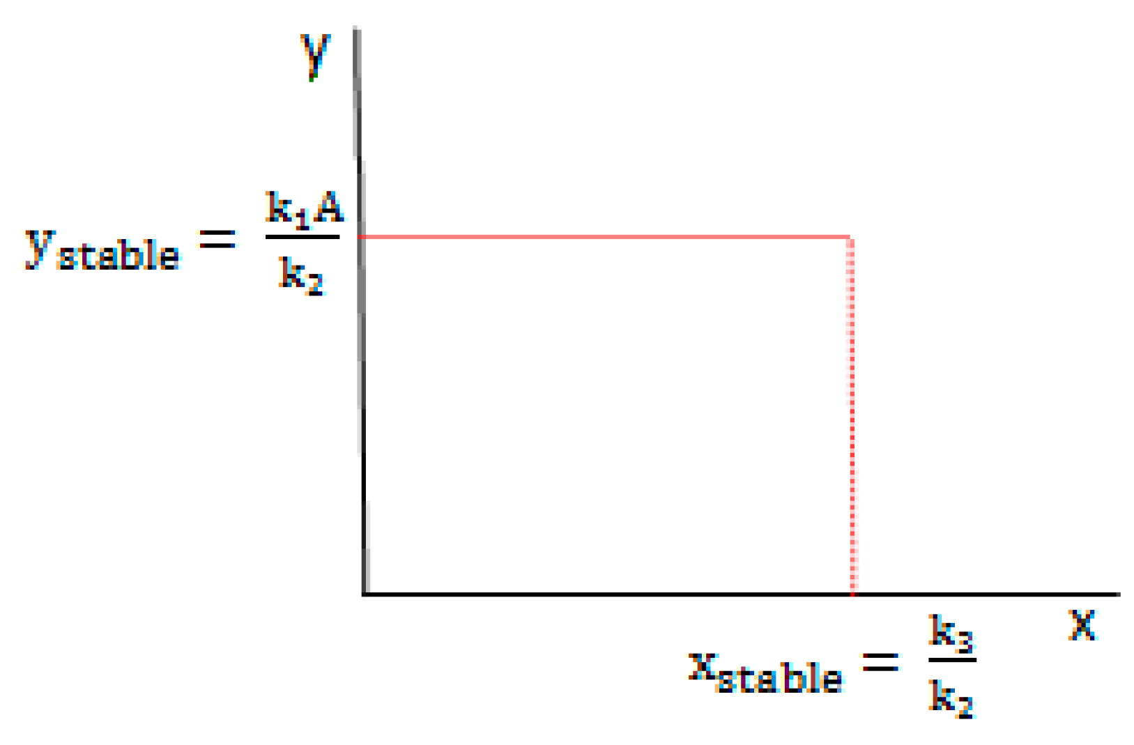
y. Focusing the study on these equations, Equations (1) and (2), at the equilibrium point, we can write
whose solutions are given by (
Figure 1),
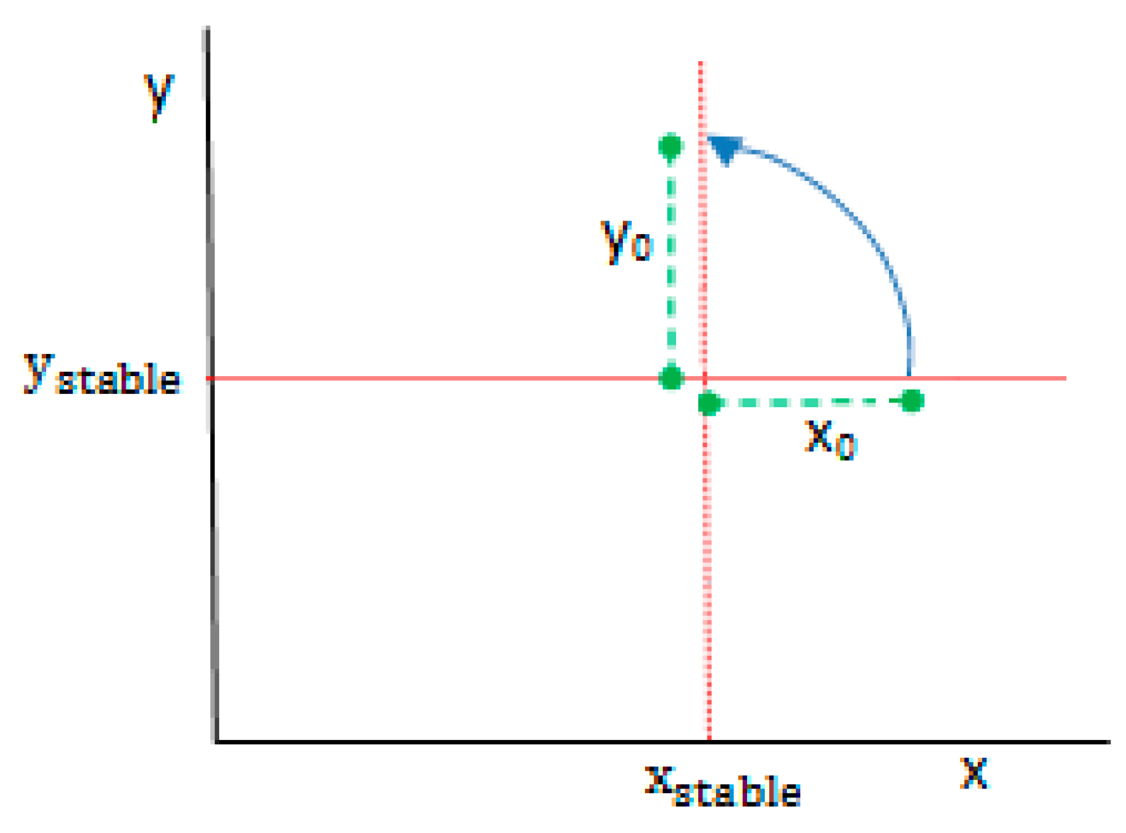
Note that in the first quadrant, due to the transformation of one species into another, the initial concentration of the species
x (
xstable +
x0) tends to reduce to a local minimum (
xstable), while species y tends to increase from its initial value (
ystable) up to a local maximum value (
ystable +
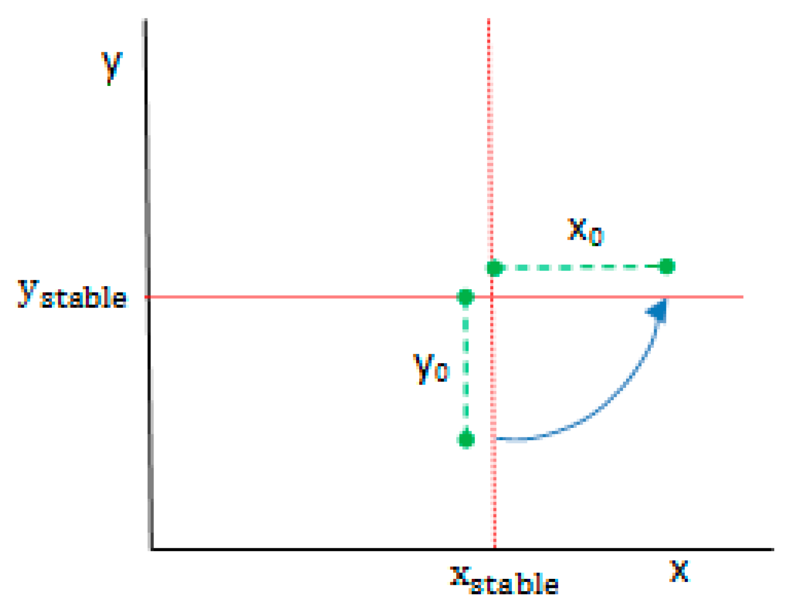
y0). Consequently, rotation of the system will be counterclockwise,
Figure 2.
In the general case, it can be assumed that the interaction between species, which depend on the parameters of the problem (Ak1, k2, and k3), consists of a cycle of increase and decrease in the concentration of both, which will be periodically repeated. Temporal representations of these concentrations will be harmonic continuous waves, with different periods of rising and falling from its stable values (xstable, ystable).
Reducing Equations (1) and (2) to their dimensionless form, which is done following a normalized nondimensionalization process of the same, we obtain the independent dimensionless groups that, based on the π-theorem, govern the solutions of the problem. To do this, two references are needed for making dimensionless variables x and y. For simplicity, we choose initial values (xi or yi) located on the lines x = xstable or y = ystable. The possible alternatives for the choice of these references (xi, yi) are (subscripts i and f mean initial and final points, respectively, of the path segment in the phase diagram):
A value for xi above xstable (xi > xstable) with yi = k1A/k2, Equation (6). Then, the trajectory from the value (xi, ystable) to (x = xstable,yf) is studied. In this process, xi is given and yf is an unknown. The time for this trajectory is also unknown.
A value for yi above ystable (yi > ystable) with xi = xstable. The trajectory goes from the value (xstable, yi) to the point (xf,y = ystable). In this process, yi is given while xf and the time required for the trajectory are unknowns.
A value for xi under xstable (xi < xstable) with yi = ystable. The trajectory goes from the value (xi, ystable) to (x = xstable,yf). xi is given while yf and the time are unknows.
A value for yi under ystable (yi < ystable) with xi = xstable. The trajectory goes from the value (xstable, yi) to the point (xf,y = ystable). yi is given while xf and the time are unknowns.
Different solutions for each of the previous cases will be provided because of no symmetry of the evolution of the species along the whole cycle. The problem is studied between two states of evolution contained in the lines x = xstable and y = ystable (one state in each line). The choice of an arbitrary starting point, where it is not contained in any of the lines x = xstable or y = ystable, is also possible. In this case, the starting point is (xi, yi) while the final, (xf, yf), is located at lines x = xstable or y = ystable, depending on the quadrant in which the starting point is located and the sense of rotation.
Let us deduce the dimensionless groups of the former alternatives:
Case (i). Locate at the first quadrant of the phase space (
Figure 2). The starting point is the maximum value of the species
x (distance
xo above the stable value
xstable). Write:
The dimensionless variables, which range in the interval [0, 1], are defined as follows:
or, reorganizing,
Replacing these variables in the governing equations and defining
to as the time elapsed between the initial and final points, the dimensionless forms of Equations (1) and (2) are deducted. On the one hand, from the dimensionless form of Equation (2), the following coefficients result:
,
−k3,
k2xo, which provide the monomials (or dimensionless groups):
On the other hand, from the dimensionless form of Equation (1), the emergent coefficients are
,
k1A, and
−k2yo, leading to the monomials
Now, manipulating groups (11) and (12) in order introduce the unknowns
yo and
to in separated monomials, we can write them in the form
From these, applying the
π-theorem, solutions for
yo and
to are obtained,
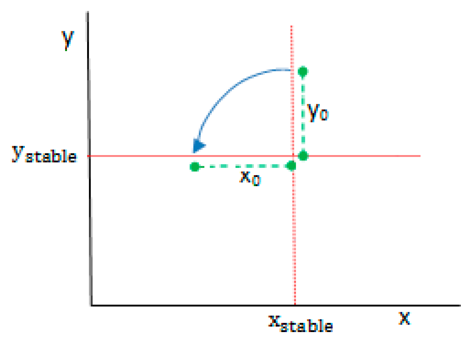
Case (ii). The phase diagram is within the second quadrant,
Figure 3. The starting point is the maximum value of the species
y (
yo+
ystable). Write:
The dimensionless variables are defined in the form
or
Proceeding as in case (i), Equation (1) provides the coefficients
,
k1A, and
−k2yo, and the monomials.
while Equation (2) gives rise to the coefficients
,
k2xo,
−k3, and to the monomials.
The final monomials can be reorganized mathematically and written in the form
providing the solutions
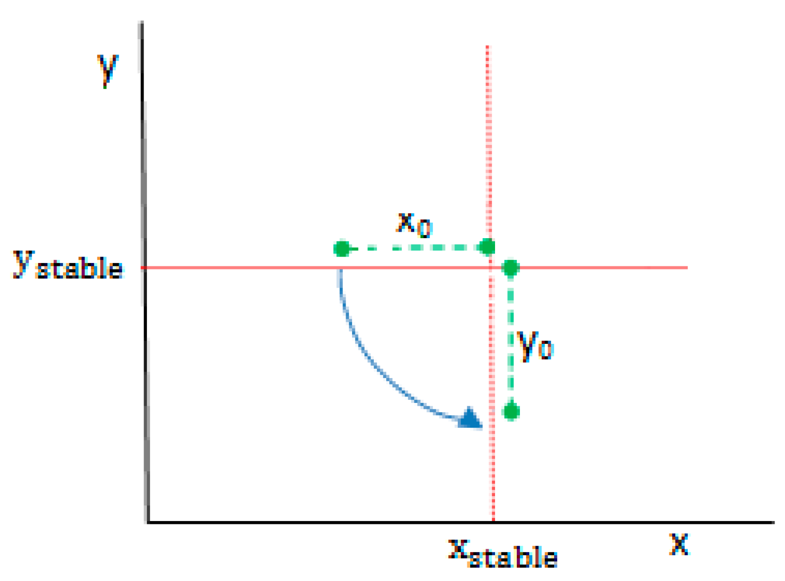
Case (iii). The path is shown in
Figure 4. Starting and final points are
These used as references provide the dimensionless variables
or
Proceeding as in the former cases, the resulting monomials can be written in the form
Thus, solutions for
to and
xo are
Case (iv). The phase space locates at the fourth quadrant,
Figure 5. The starting point is the minimum value of the species
y (
ystable −
yo). The references are now:
Final point:
while dimensionless variables are defined in the form
or
Replacing these expressions in the governing equations, the resulting monomials are:
Provide the solutions for
to and
xo 3. Verification of Results
In order to check the accuracy and reliability of the expressions deduced for unknowns in the four paths of the former section, we numerically simulate the set of twelve scenarios shown in
Table 1. These scenarios are grouped in four cases, with three scenarios in each case. The first scenario of each case is chosen as a basis in order to be compared to the other two simulations. The procedure may be summarized in two steps:
Firstly, values are assigned to the parameters Ak1, k2, k3, xi, yi, and xo for cases (i) and (iii), and yo for cases (ii) and (iv).
Secondly, these values are suitably changed in such a way that the dimensionless groups involved in each case retain the same value. Therefore, the arguments of the functions from which the unknowns to and yo (or xo) depend do not change, and neither do the functions themselves.
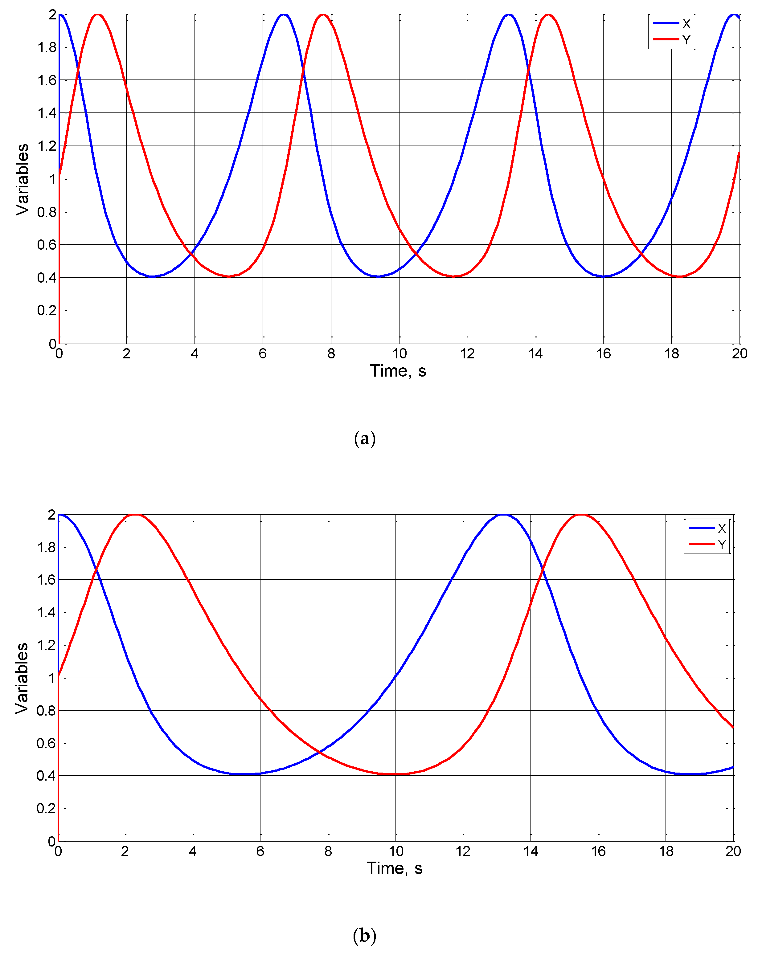
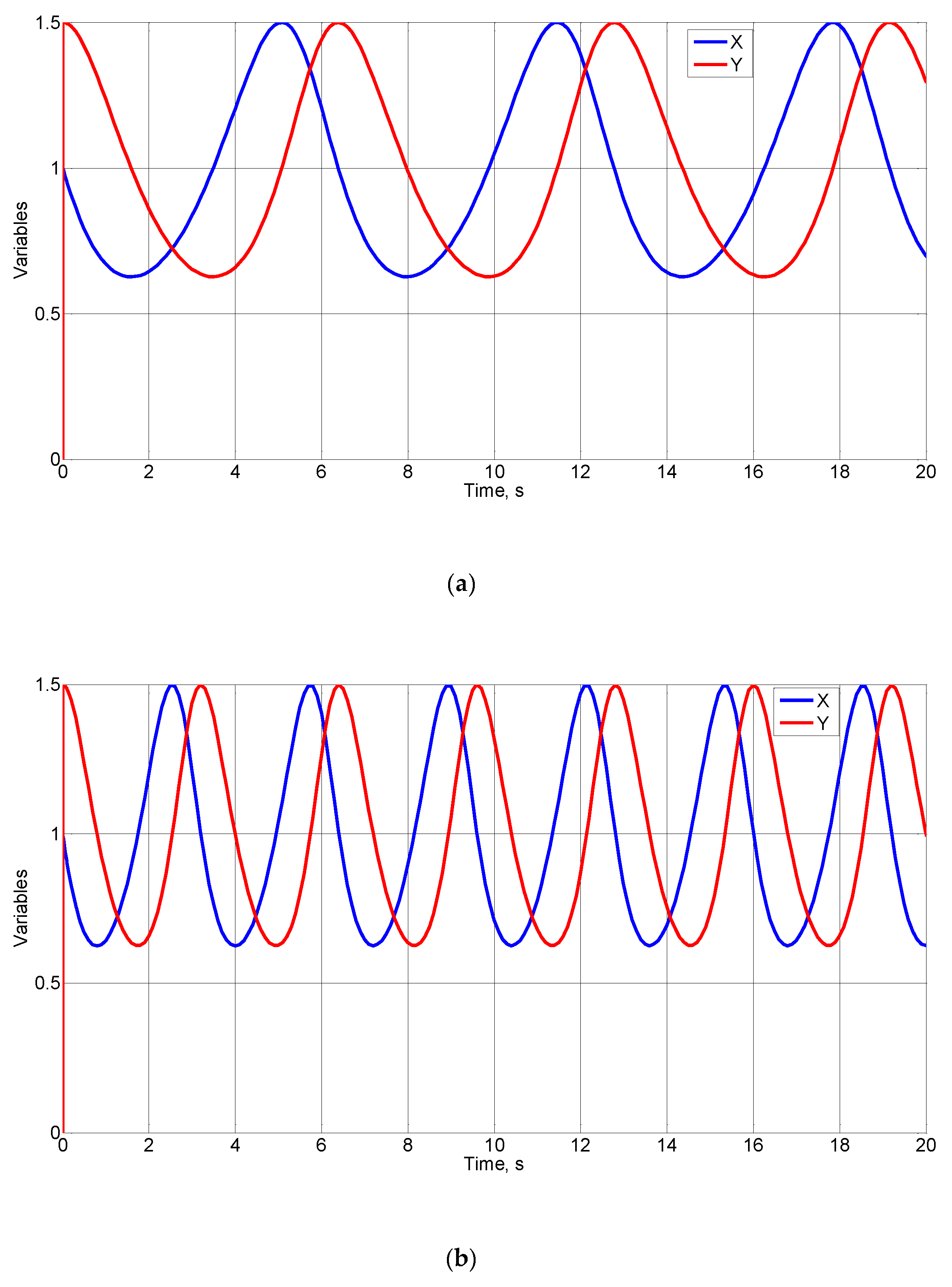
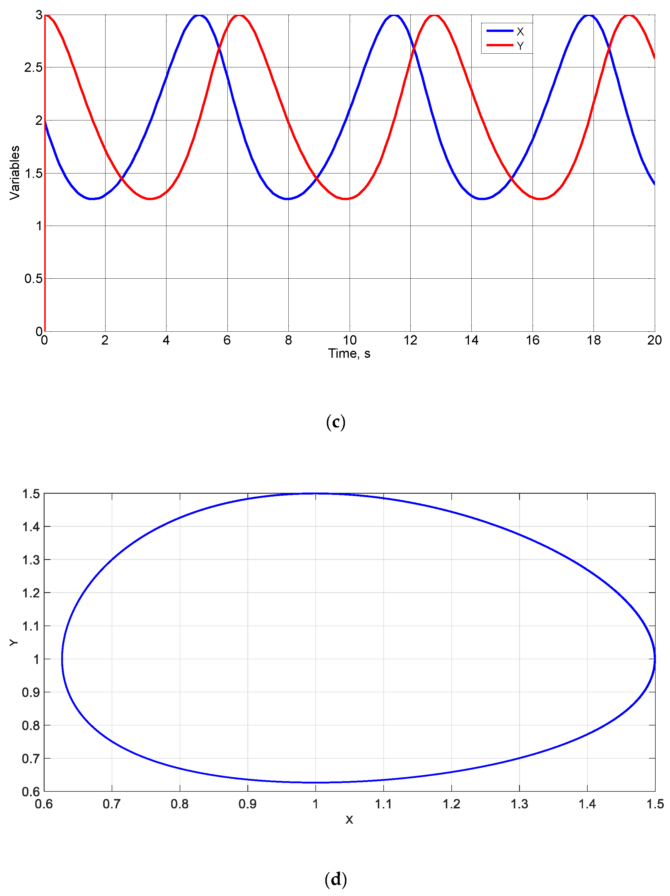
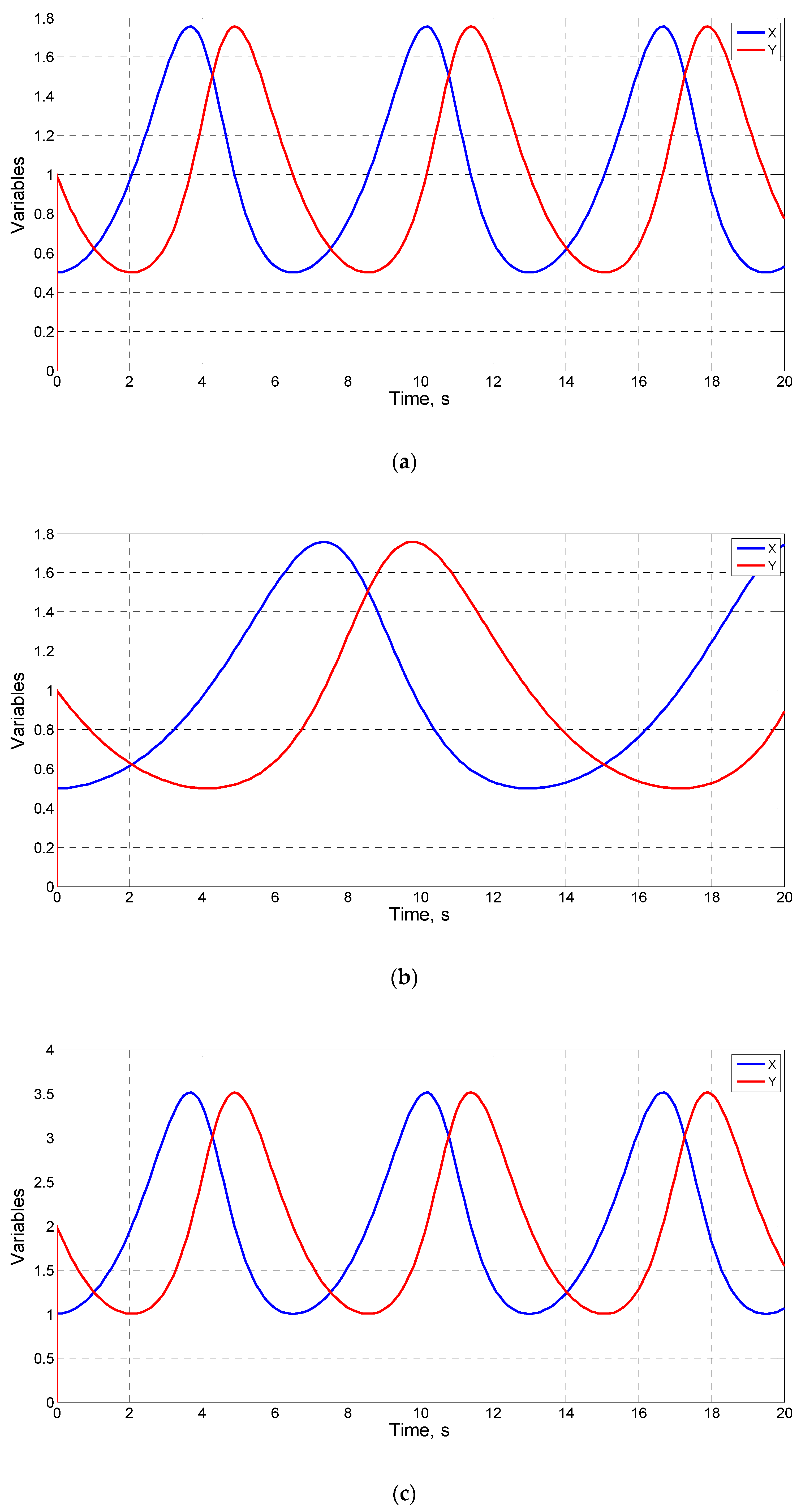
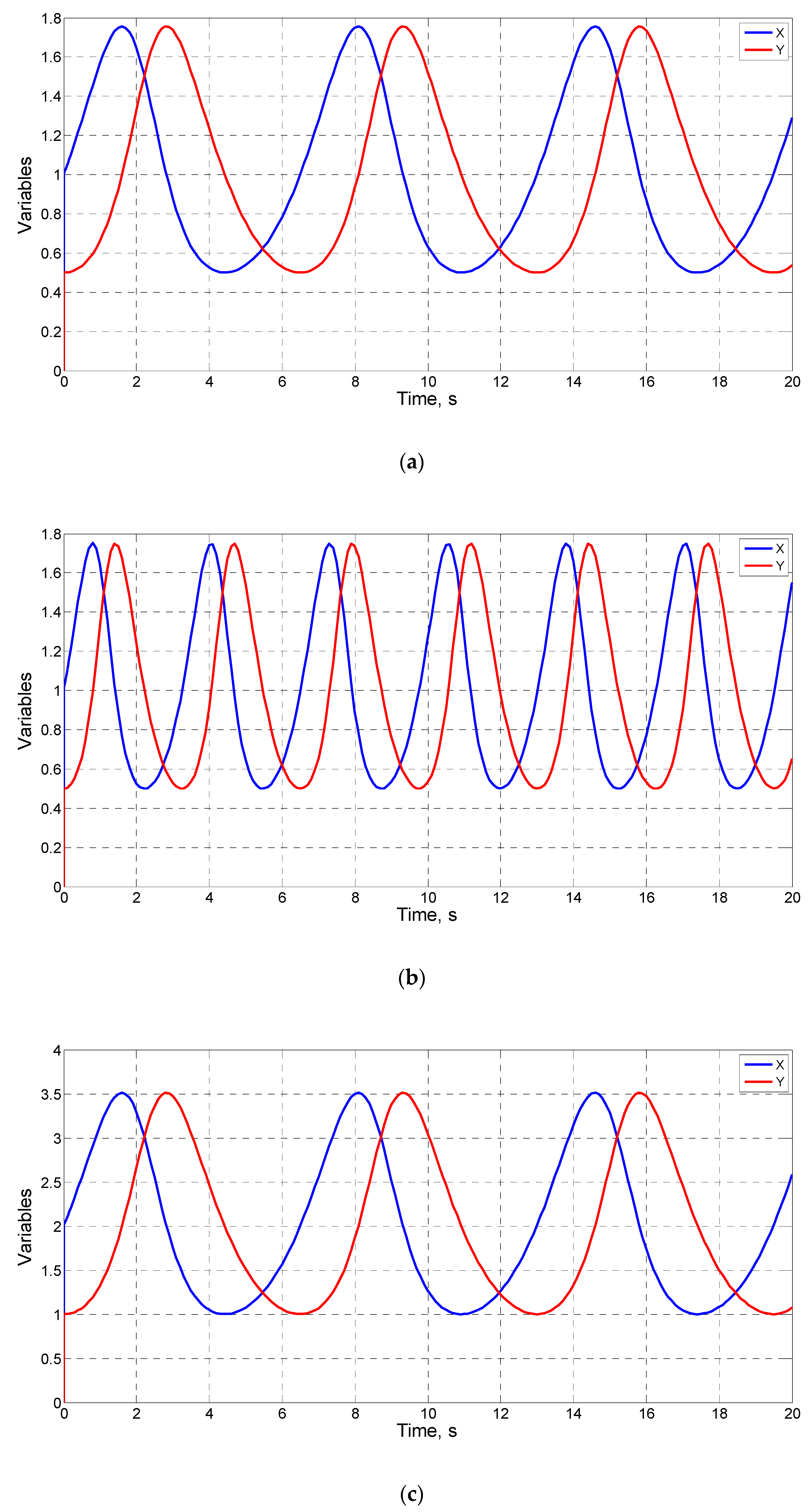
Table 1 shows the values of the parameters of each scenario. Solutions for
xo and
to in cases (ii) and (iv), respectively, and
yo and
to in cases (i) and (iii), respectively, read from the simulations (
Figure 6,
Figure 7,
Figure 8 and
Figure 9), are included in the last columns of the table. Note that, for example, in case (i),
yo duplicates in the third scenario (in comparison to the first scenario) due to the parameter
k2 being halved. By contrast, in the second scenario,
to is doubled by the effect of halving
k3, while
yo does not change. Similar comments can be made for the rest of the simulations in the table.
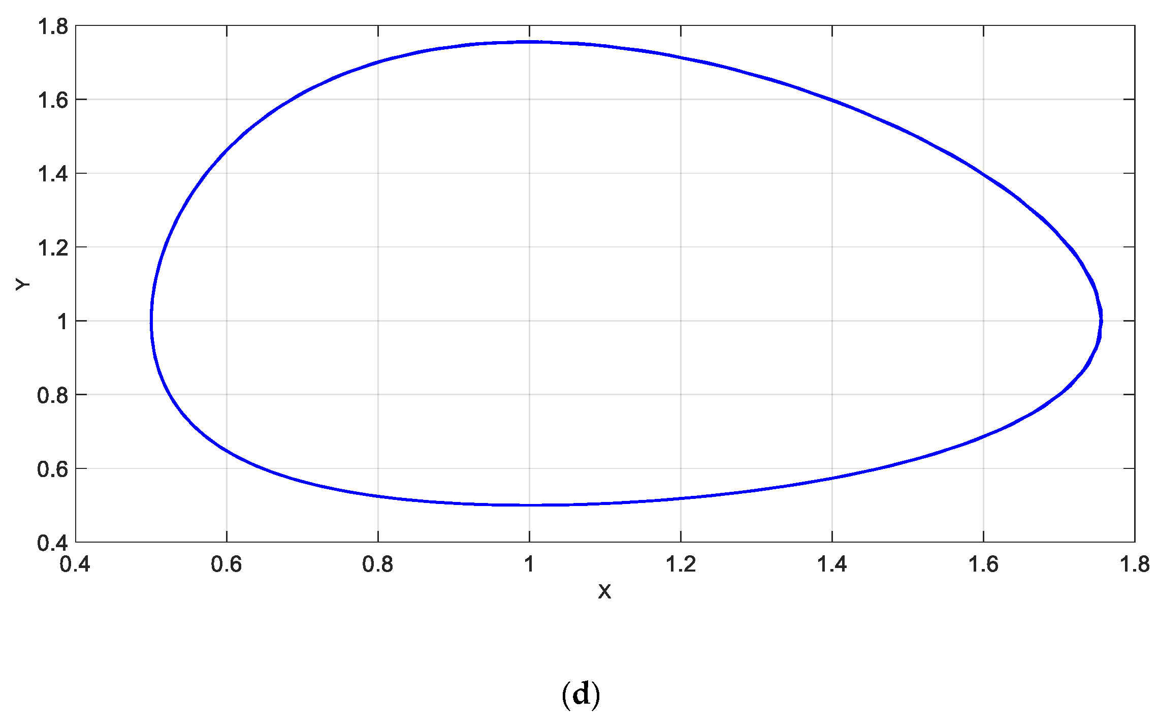
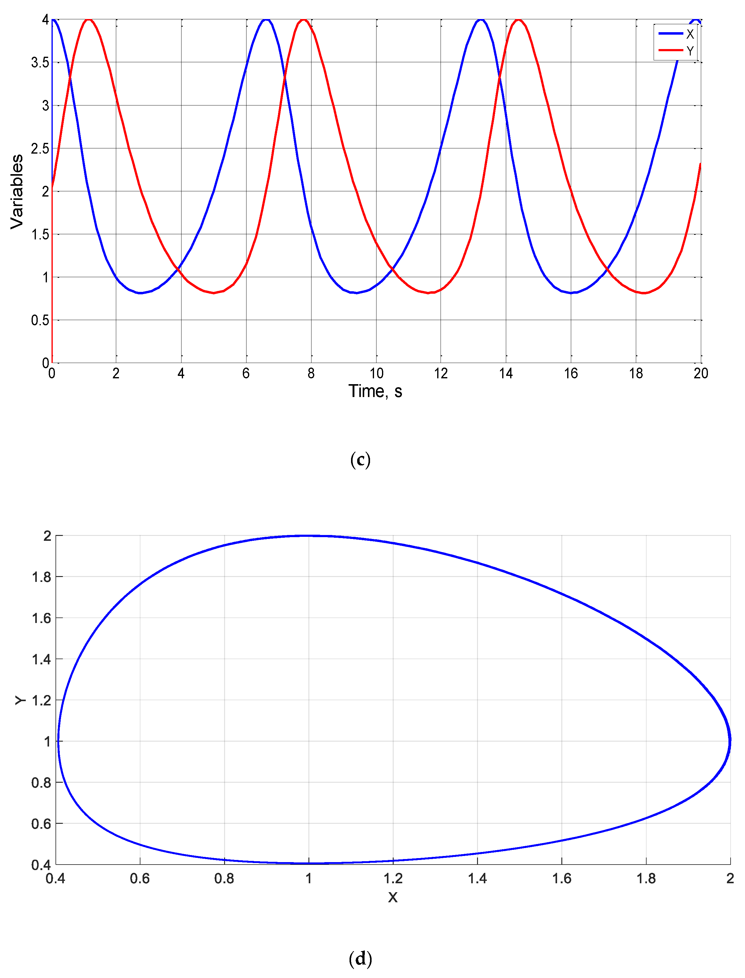
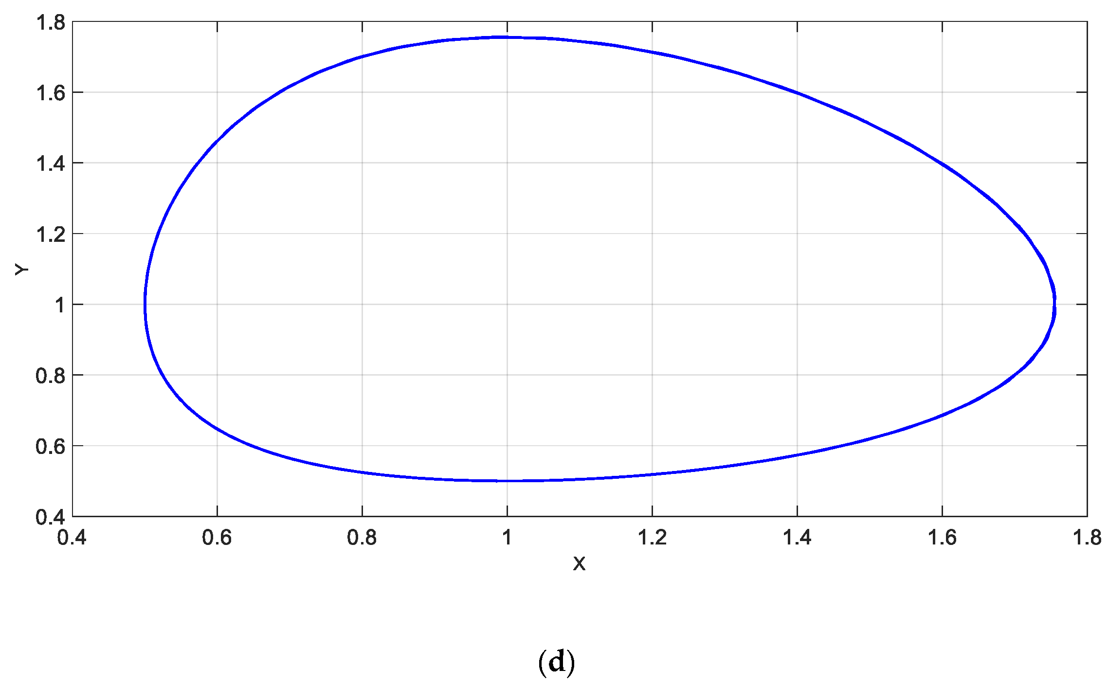
Figure 6,
Figure 7,
Figure 8 and
Figure 9 show the harmonic evolution of species and allow
to to be read for each scenario. Phase diagrams are also shown in the figures.
It is clear that the dependences between unknowns and parameters (or monomials), Equations (14) and (15) for case (i), (23) and (24) for case (ii), (30) and (31) for case (iii), and (37) and (38) for case (iv), leads to a different time t
o for each one of the quadrant, a solution that clearly emerges from the simulations. Note, however, that the solutions for
to can also be made in the same form for the four cases by simple mathematical manipulation. In effect, the solutions
for cases (i) and (iii) and
for cases (ii) and (iv) are interchangeable. This means that the total period of a complete cycle of the problem (
To), the sum of the four times of each quadrant, is also dependent on the same monomials:
4. Final Comments and Conclusions
The normalized nondimensionalization of a system of two coupled ordinary differential equations (that represent problems of interactions between species type Lotka–Volterra) has been a relatively quick and reliable procedure that allows one to obtain the dimensionless groups that rule the solution of these problems. From these groups and applying the π-theorem, the order of magnitude of some unknowns of interest can also be determined. To transform the governing equations into their dimensionless form, we only need simple mathematical manipulations; however, to choose the appropriate reference values that make the independent and dependent variables of equations dimensionless, an in-depth understanding of the physical or chemical processes involved has been required.
A general conclusion can be observed regarding the large variety of possible references for the independent and dependent variables. The references for a specific variable should not necessarily be the same in each equation of the system nor in the analysis of the solution of each quadrant of the phase diagram. In the Lotka–Volterra system under study, we have several references for concentrations as there are initial values, as well as the stable point concentrations. In addition, normalization of the dimensionless variables, which range in the interval [0, 1], imposes new restrictions for the choice of reference values. Furthermore, due to the nonlinearity of the problem, the characteristic time has been defined for each portion of the quadrant of the diagram phase in order to obtain the dependence of these partial times on the dimensionless groups of the problem. Even if the times depend on the same groups, the unknown functions of the arguments (monomials) are not necessarily the same, so the times are of the same order of magnitude but not of the same value. In addition, the period corresponding to a whole cycle (which obviously depends on the same dimensionless groups) has not been obtained directly but as a sum of the times related to the four quadrant trajectories. Overall, it is shown that the procedure used in this work gives rise to very valuable information about the solutions of a complex phenomenon, just with a little mathematical effort.
In view of the results, the normalized nondimensionalization procedure applied in this work opens two perspectives: (a) The construction of universal abacuses that represent the unknowns of interest as a function of the dimensionless groups, on the one hand (a result derived from the π- theorem); for this end, a large number of numerical solutions is required. (b) The application of the procedure to systems with more than two variables, on the other hand. However, as the number of parameters increases significantly with the number of variables, the complexity of the study increases greatly due to the existence of different periods in each phase diagram.


