Entrainment of Weakly Coupled Canonical Oscillators with Applications in Gradient Frequency Neural Networks Using Approximating Analytical Methods

Abstract

Solving phase equations for systems with high degrees of nonlinearities is cumbersome. However, in the case of two coupled canonical oscillators, that is, a reduced model of translated Wilson–Cowan neuronal dynamics, under slowly varying amplitude and rotating wave approximations, we suggested a convenient way to find their average relative phase evolution. This approach enabled us to find an explicit solution for the average relative phase of the two coupled canonical oscillators based on the original neuronal model parameters, and importantly, to find their phase-locking constraint. This methodology is straightforward to implement in any Wilson–Cowan-type coupled oscillators with applications in gradient frequency neural networks (GFNNs).

1. Introduction

Complex systems transit between various dynamical states. The overall dynamical description of a complex system in many cases can be reduced to a low-dimensional set of nonlinear ordinary differential equations [1]. In cases of a biological complex system, for instance, a nervous system, the descriptive dynamical models could be a Hodgkin–Huxley model that gives a detailed biophysical description of action potential initiation and propagation in neurons, and a Wilson–Cowan neural mass model that describes the dynamics of excitatory and inhibitory neural populations. However, it is rare or even impossible to know precisely all the parameters that are employed in these types of models. To address this issue, one can utilize model reduction techniques to obtain a canonical description of the main models. A canonical model is the simplest class of equivalent dynamical models in analytical terms, and can be derived by methods such as normal form and center manifold theory. For example, the simple spiking model of Izhikevich is a canonical model of Hodgkin–Huxley that could be obtained by either nullclines or current-voltage relations. The canonical model approach is useful for studying the behavior of the entire family of models if the information about most of their parameters is not complete or well known [2].

The canonical model for gradient frequency neural networks (GFNNs) or in short, the canonical model, is a simplified mathematical model that describes the dynamical properties of oscillatory neural populations near a Poincaré-Andronov-Hopf bifurcation [3,4]. Models of cochlear outer hair cells assume critical oscillations based on Hopf bifurcation. For example, it is proposed that in the mammalian cochlea, the basilar membrane is driven by a set of critical oscillators (most likely outer hair cells) and the response of a critical Hopf oscillator has considerable bearing on human psychoacoustics [5]. The canonical model is capable of processing time varying external stimuli, and facilitates the study of nonlinear time-frequency transformations [3], which is important in auditory signal processing. Bifurcation analysis and dynamical properties of a periodically-forced canonical oscillator have been investigated in detail [4]. Such analysis is of importance because the canonical model describes the state transitions of the system between quiescence and spontaneous activity. However, finding the analytical solutions of a canonical model that contains a high amount of nonlinearity is cumbersome. Investigators have introduced and applied approximating analytical methods such as the homotopy perturbation method [6,7], the variational iteration method and more [8]. In this manuscript, we study the average relative phase dynamics of two coupled canonical oscillators while utilizing slowly varying amplitude and rotating wave approximations [9].

Normal form theory, along with center manifold theory, are two approaches that mathematicians employ to simplify dynamical systems. Both of these approaches reduce dimensionality and eliminate the nonlinearities up to the desired order. The method of normal forms can be traced back to the Ph.D. thesis of Henri Poincaré (1929) [10]. It is a powerful tool with which to study the stability and bifurcation analysis of nonlinear differential equations, which employs successive, near-identity nonlinear transformations to obtain a simple form and is restricted to systems which do not have perturbation parameters (unfoldings) [11]. The structure of normal forms is determined entirely by the linear part of the vector field under study. Here we employ conventional normal form theory (CNF), which uses the near-identity change of variables to find the canonical models of single and coupled Wilson–Cowan oscillators.

Our analysis in this paper is categorized under four sections. In Section 2.1 that forms an overview, we start with a Wilson–Cowan oscillator and obtain its normal form. Then we restate the theorems that facilitate deriving a canonical model for single Wilson–Cowan oscillators (the canonical model). In Section 2.2 we extend the methodology of the near-identity change of variables in normal form theory for single oscillators of Section 2.1 to obtain a canonical model for two coupled Wilson–Cowan oscillators. By utilizing polar transformation and decomposing the real and imaginary parts of the system, we obtain radial and angular equations of motion for each of the canonical oscillators. These equations are highly nonlinear and not straightforward to solve analytically. We propose an ansatz in Section 3 that is valid under slowly varying amplitude and rotating wave approximations and leads to a dynamical description of the average relative phase between the two coupled canonical oscillators. This proposed method facilitates working with the cumbersome radial and angular equations derived in Section 2.2. Finally, we solve the average relative phase equation explicitly. This solution is validated by taking its time limit to check if we have correctly obtained the steady state.

2. Methods

2.1. The Canonical Model of Single Oscillators

2.1.1. Wilson–Cowan Model

The Wilson–Cowan model is a model of neural oscillation based on excitatory and inhibitory neural populations. Neurons are called excitatory if they increase the probability of a postsynaptic action potential occurring, and inhibitory if they decrease this likelihood. According to Hugh D. Wilson and Jack D. Cowan, all nervous processes of any complexity are dependent upon the interaction of excitatory and inhibitory cells [12]. Consider an interconnected pair of excitatory and inhibitory neurons. This pair is called a Wilson–Cowan neural oscillator, and is considered one of the basic mechanisms of the generation of oscillatory activity in the brain [13]. Each unit in the oscillator represents a local population of neurons, in the cerebellum, olfactory cortex and neocortex. By letting $x_i$ and $y_i$ denote activity of the ith excitatory and inhibitory neurons, respectively, the Wilson–Cowan neural model has the form:

$$\begin{array}{c}\hfill {\mu }_x\dot{x_i}=-x_i+(1-{\tau }_x{x}_i)S({\rho }_{x_i}+\sum _{j=1}^n{a}_{ij}{x}_j-\sum _{j=1}^n{b}_{ij}{y}_j)\\ \hfill {\mu }_y\dot{y_i}=-y_i+(1-{\tau }_y{y}_i)S({\rho }_{y_i}+\sum _{j=1}^n{c}_{ij}{x}_j-\sum _{j=1}^n{d}_{ij}{y}_j)\end{array}$$

(1)

where ${\mu }_x$ and ${\mu }_y>0$ are the membrane time constants and ${\tau }_x$ and ${\tau }_y$ are refractory periods of excitatory and inhibitory neurons, respectively. $a_{ij}$, $b_{ij}$, $c_{ij}$ and $d_{ij}>0$ for $i\ne j$ are synaptic coefficients. $b_{ii}$ and $c_{ii}$ are synaptic too, since they denote interactions between excitatory and inhibitory neurons within the ith neural oscillator. $a_{ii}$ and $d_{ii}$ are feedback parameters, which can be positive or negative. Parameters ${\rho }_{x_i}$ and ${\rho }_{y_i}$ denote the external inputs from sensory organs and other regions of the brain to the ith excitatory and inhibitory neurons respectively. S is a sigmoid function that is continuous and monotonously increases. For simplicity and without loss of generality, we consider the Wilson–Cowan neural model in the special case ${\tau }_x={\tau }_y=0$ and ${\mu }_x={\mu }_y=1$. That is:

$$\begin{array}{c}\hfill \dot{x_i}=-x_i+S({\rho }_{x_i}+\sum _{j=1}^n{a}_{ij}{x}_j-\sum _{j=1}^n{b}_{ij}{y}_j)\\ \hfill \dot{y_i}=-y_i+S({\rho }_{y_i}+\sum _{j=1}^n{c}_{ij}{x}_j-\sum _{j=1}^n{d}_{ij}{y}_j)\end{array}$$

(2)

We first derive the canonical model for single translated Wilson–Cowan oscillator without external inputs, ${\rho }_x={\rho }_y=0$ in Equation (2):

$$\begin{array}{c}\hfill \dot{x}=-x+tanh(ax-by)\\ \hfill \dot{y}=-y+tanh(cx-dy)\end{array}$$

(3)

Third-order Taylor expansion of the hyperbolic tangent function in Equation (3) leads to the translated Wilson–Cowan model expanded to cubic order:

$$\begin{array}{c}\hfill \dot{x}=(a-1)x-by-ax(\frac{a^2{x}^2}{3}+b^2{y}^2)+by(\frac{b^2{y}^2}{3}+a^2{x}^2)\\ \hfill \dot{y}=-(d+1)y+cx+dy(\frac{d^2{y}^2}{3}+c^2{x}^2)-cx(\frac{c^2{x}^2}{3}+d^2{y}^2)\end{array}$$

(4)

Our strategy in this study (via CNF) is based on the fact that changing the coordinates must not affect the stability of the origin. In fact, we only use coordinate transformations that map the origin to itself.

2.1.2. The Normal Form

Locality, the inclusion of nonlinear transformations and the dominance of the linear part of the system are three requirements of normal form theory [10]. In other words, nonlinear coordinate transformations (near-identity change of variables) are to be performed in the vicinity of a fixed point (in case of Equation (4), the origin), and the structure of this normal form is determined entirely by the linear part of the system under study.

To find the normal form of Equation (4), we map the Cartesian coordinates $(x,y)$ on the complex domain by introducing $s=x+iy$ and $\overline{s}=x-iy$. By differentiating s with respect to time and substituting for $\dot{x}$ and $\dot{y}$ given in Equation (4) we get:

$$\begin{array}{cc}\hfill \dot{s}& =\dot{x}+i\dot{y}\hfill \\ \hfill & =\left(\frac{a-1+ic}{2}\right)\left(s+\overline{s}\right)+\left(\frac{-1-d+bi}{2}\right)\left(s-\overline{s}\right)\hfill \\ \hfill & -\frac{a^3}{24}{\left(s+\overline{s}\right)}^3+\frac{b^3}{24}i{\left(s-\overline{s}\right)}^3\hfill \\ \hfill & +\left(\frac{a{b}^2+ic{d}^2}{8}\right)\left(s+\overline{s}\right){\left(s-\overline{s}\right)}^2\hfill \\ \hfill & +\left(\frac{c^{2}d-i{a}^{2}b}{8}\right){\left(s+\overline{s}\right)}^2\left(s-\overline{s}\right).\hfill \end{array}$$

(5)

We have used the fact that $x=\frac{s+\overline{s}}{2}$ and $y=\frac{s-\overline{s}}{2i}$. Now, we perform a near-identity change of variables, i.e., substitute for s by z according to the transformation:

$$s⟼z+\kappa z^p{\overline{z}}^q,$$

(6)

where p and q are positive integers whose sum gives us the highest order of nonlinearity present in the desired canonical model and $\kappa$ is a complex number. This is an essential step in the normal form theory which gives us the chance to eliminate the desired terms by setting $\kappa$ appropriately, and consequently simplify the model in terms of nonlinear terms present in the expansion. Finding such values for $\kappa$ is presented in Appendix A. Rearranging Equation (6) in terms of z yields:

$$\begin{array}{cc}\hfill z& =s-\kappa z^p{\overline{z}}^q\hfill \\ \hfill & =s-\kappa {(s-\kappa z^p{\overline{z}}^q)}^p{(\overline{s}-\overline{\kappa }{\overline{z}}^p{z}^q)}^q\hfill \\ \hfill & =s-\kappa s^p{\overline{s}}^q+\dots .\hfill \end{array}$$

(7)

If we differentiate this equation with respect to time, we get an expression for $\dot{z}$ that without considering quintic and higher terms ($p+q=3$) is:

$$\dot{z}=\dot{s}-p\kappa s^{p-1}\dot{s}{\overline{s}}^q-q\kappa s^p\dot{\overline{s}}{\overline{s}}^{q-1}.$$

(8)

There are two choices for p and q, either $(p,q)=(1,2)$ or $(p,q)=(2,1)$. Both cases are presented in Appendix A, along with detailed calculations. In either case, the general normal form of Wilson–Cowan model (Equation (3)) can be expressed as:

$${\dot{z}}_s=A_{1}z+A_2\overline{z}+A_{pq}{z}^p{\overline{z}}^q$$

(9)

with the coefficients presented in Appendix A. We replaced $\dot{z}$ by ${\dot{z}}_s$ to indicate that this normal form is for a single oscillator. This CNF can describe all kinds of bifurcations.

2.1.3. The Normal Form about a Hopf Bifurcation Point: The Canonical Model

Here we utilize two theorems from local dynamical systems theory [10] to reduce the normal form in Equation (9) into the canonical model, the model that describes the system about a Hopf bifurcation point.

Note that in the near-identity change of variables we made a transformation of the form $z⟼z+h(z,\overline{z})$ where h is third-order in z and $\overline{z}$.

Theorem 1.

In transformations of the type $z⟼z+h(z,\overline{z})$ for some $h=z^p{\overline{z}}^q$ at the bifurcation point of Hopf type we must not have $p-q=-1$ [10].

This can never happen if p and q are both even numbers. Therefore, all even-order terms can be removed from the expansion. This theorem guarantees that even if the expansion of the sigmoid function S contains even-order terms, they can be removed for the special case of Hopf bifurcation. This condition also suggests that it works only with $p=2$ and $q=1$, so Equation (9) can be written as:

$$\dot{z}=A_{1}z+A_2\overline{z}+A_{21}{z}^2\overline{z}.$$

(10)

This is still not the simplest normal form of Hopf bifurcation.

Theorem 2.

The cubic terms except $z^2\overline{z}$ can be eliminated for the Hopf normal form [10].

This is true if and only if:

$$A_2=\frac{a+d}{2}+\frac{1}{2}i(-b+c)=0$$

(11)

which means $a=-d$ and $b=c=\omega$ where $\omega$ is a real number. Substituting these results in the other coefficient $A_1$ leads us to:

$$A_1=\frac{1}{2}(-2+a-d)+i\left(\frac{b+c}{2}\right)=(a-1)+i\omega .$$

(12)

By introducing $\alpha =a-1$ and $\beta =A_{21}$, Equation (10) becomes:

$$\dot{z}=(\alpha +i\omega )z+\beta z^2\overline{z}.$$

(13)

This is the canonical model for a single Wilson–Cowan oscillator without external input in agreement with the results in [13]. In other words, the canonical model (Equation (13)) is the description of a Wilson–Cowan oscillator (Equation (3)) about a Hopf bifurcation point. We compare the nullclines of the translated Wilson–Cowan oscillator with the ones obtained by the canonical model (set $\dot{z}=0$ in Equation (13)) in Figure 1. The nullclines of the models coincide in the vicinity of the origin (the fixed point), which is the point of interest.

2.2. The Canonical Model of Two Coupled Oscillators

Now we consider two isolated Wilson–Cowan oscillators that are coupled. We write down synaptic and feedback parameters as follows:

$$\begin{array}{c}\hfill a_{11}=a_{22}=a,b_{11}=b_{22}=b,c_{11}=c_{22}=c,d_{11}=d_{22}=d,\\ \hfill a_{12}=a_{21}=s_1,b_{12}=b_{21}=s_2,c_{12}=c_{21}=s_3,d_{12}=d_{21}=s_4\end{array}$$

Additionally, we assume there are no external stimuli to the system, so ${\rho }_{x_1}={\rho }_{x_2}=0$. Assuming above conditions in Equation (2) leads to:

$$\begin{array}{c}\hfill \dot{x_1}=-x_1+S(a{x}_1-b{y}_1+w_1{x}_2-w_2{y}_2)\\ \hfill \dot{y_1}=-y_1+S(c{x}_1-d{y}_1+w_3{x}_2-w_4{y}_2)\\ \hfill \dot{x_2}=-x_2+S(a{x}_1-b{y}_1+w_1{x}_2-w_2{y}_2)\\ \hfill \dot{y_2}=-y_2+S(c{x}_1-d{y}_1+w_3{x}_2-w_4{y}_2)\end{array}$$

(14)

For small synaptic coefficients $w_1,..,w_4$, i.e., to the order of $ϵ\ll 1$, we can rescale the system as $w_k=ϵc_k$ for $k=1,2,3,4$. By choosing tanh as the sigmoidal function S and rescaling, the translated Wilson–Cowan model for two coupled identical oscillators is described by [13]:

$$\begin{array}{c}\hfill \dot{x_1}=-x_1+tanh(a{x}_1-b{y}_1)+ϵsec{h}^2(a{x}_1-b{y}_1)(c_1{x}_2-c_2{y}_2)\\ \hfill \dot{y_1}=-y_1+tanh(c{x}_1-d{y}_1)+ϵsec{h}^2(c{x}_1-d{y}_1)(c_3{x}_2-c_4{y}_2)\\ \hfill \dot{x_2}=-x_2+tanh(a{x}_2-b{y}_2)+ϵsec{h}^2(a{x}_2-b{y}_2)(c_1{x}_1-c_2{y}_1)\\ \hfill \dot{y_2}=-y_2+tanh(c{x}_2-d{y}_2)+ϵsec{h}^2(c{x}_2-d{y}_2)(c_3{x}_1-c_4{y}_1)\end{array}$$

(15)

2.2.1. The General Normal Form

As we did in Section 2.1, we expand the tanh functions to cubic terms for both oscillators and write the dynamics of each oscillator $(i=1,2)$ in the complex domain:

$$\dot{s_i}=\dot{x_i}+i\dot{y_i}.$$

(16)

The expansion of Equation (16) leads to some terms that describe inherent dynamics of each oscillator $\left({\dot{s_i}}_s\right)$ and other coupling terms $\left({\dot{s_i}}_c\right)$, which are addressed in details in Appendix B. So in brief:

$$\dot{s_i}={\dot{s_i}}_s+ϵ{\dot{s_i}}_c.$$

(17)

By doing a near-identity change of variables:

$$s_i⟼z_i+{\kappa }_i{z}_i^m{\overline{z_i}}^n,$$

(18)

where m and n are positive integers that satisfy $m+n=3$, we obtain the final normal form of these two coupled oscillators:

$$\dot{z_i}={\dot{z_i}}_s+ϵ{\dot{z_i}}_c.$$

(19)

Some lengthy but straightforward algebra leads to four cases for ${\dot{z_i}}_c$ depending on the values of $p,q,m$ and n, which is completely presented in Appendix B. The two cases for ${\dot{z_i}}_s$ have been already presented in Section 2.1.

2.2.2. Hopf Normal Form: The Canonical Model

As we argued in Section 2.1, Theorem 1, that at the bifurcation point we must not have $m-n=-1$. Thus, among all four choices of $p,q,m$ and n (presented as four cases in Appendix B), only the case for $p=m=1$ and $q=n=2$ is acceptable for representing Hopf bifurcation (case $\left(I\right)$ in Appendix B). Therefore, the full canonical model that exhibits Hopf bifurcation for two coupled identical Wilson–Cowan oscillators about the fixed point up to quintic terms is:

$$\begin{array}{c}\hfill \dot{z_i}={\dot{z_i}}_s+ϵ{\dot{z_i}}_c=\\ \hfill & A_1{z}_i+A_{21}{z}_i^2\overline{z_i}\hfill \\ \hfill & +ϵ[B_1{z}_j+B_2\overline{z_j}+B_5{z}_i^2{z}_j+B_6{z}_i^2\overline{z_j}\hfill \\ \hfill & +(B_7-2{\kappa }_i\overline{B_2})z_i{z}_j\overline{z_i}+(B_3-B_1{\kappa }_i)z_j{\overline{z_i}}^2\hfill \\ \hfill & +(B_8-2{\kappa }_i\overline{B_1})z_i\overline{z_i}\overline{z_j}+(B_4-B_2{\kappa }_i){\overline{z_i}}^2\overline{z_j}\hfill \\ \hfill & +B_1{\kappa }_j{z}_j{\overline{z_j}}^2+B_2\overline{{\kappa }_j}{z}_j^2\overline{z_j}]\hfill \end{array}$$

(20)

where $i\ne j$ and all coefficients $A_{21},B$ and $A_k,B_k$ for $k=1,2,\dots ,8$ depend on synaptic and feedback parameters described in the original Wilson–Cowan model in Section 2.1.1 and rephrased in Section 2.2 for the case of two coupled oscillators. All the coefficients have been calculated and are presented in Appendix A and Appendix B.

2.2.3. Radial and Angular Equations

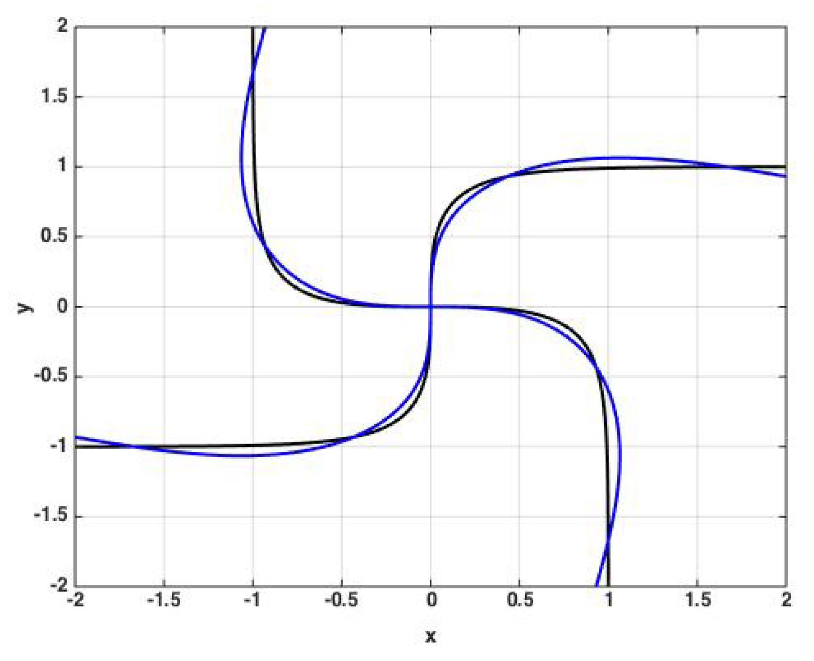
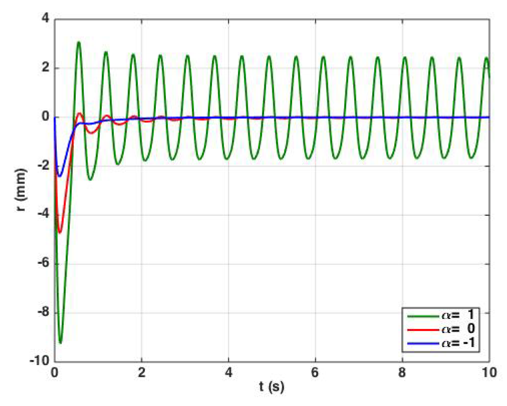
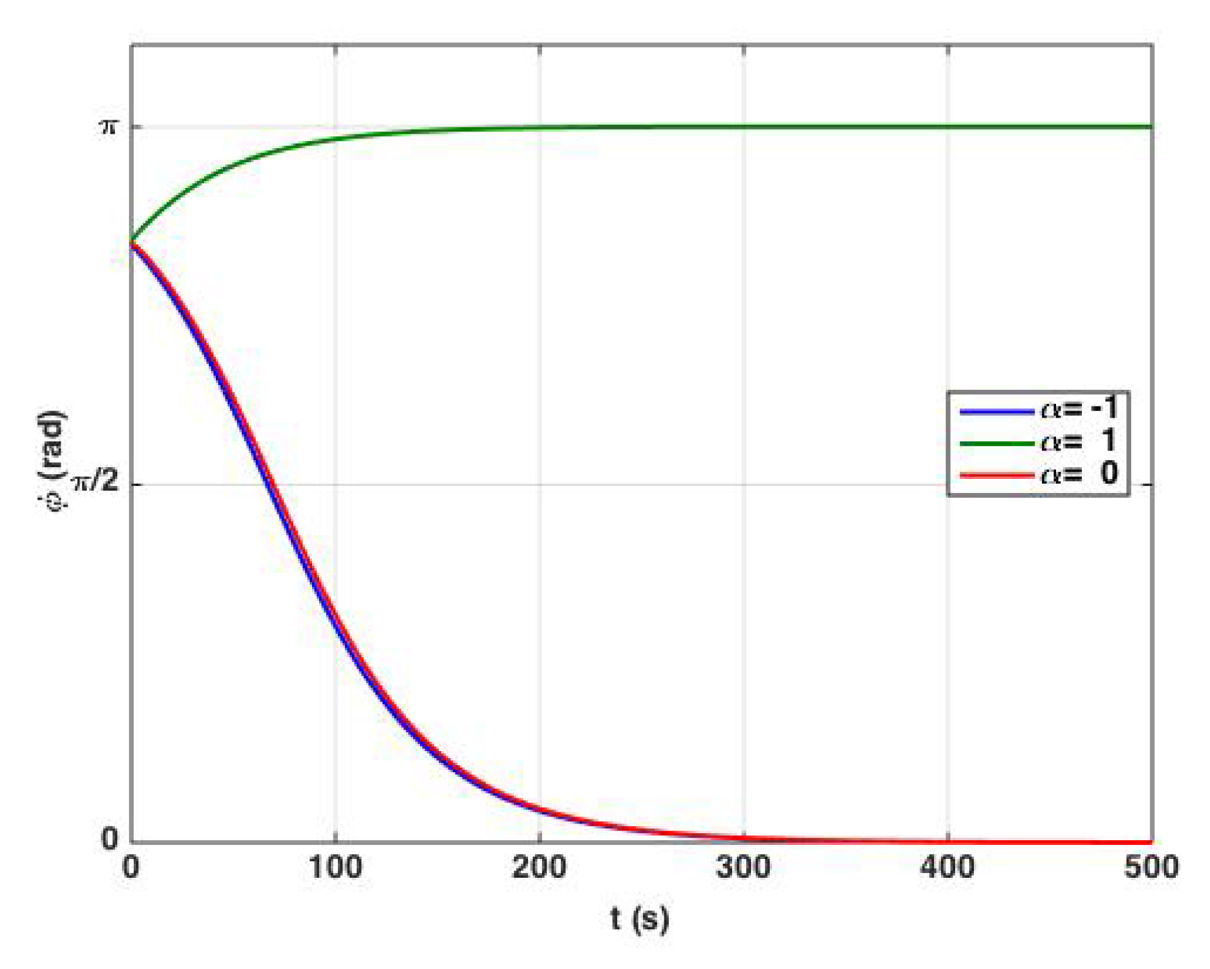
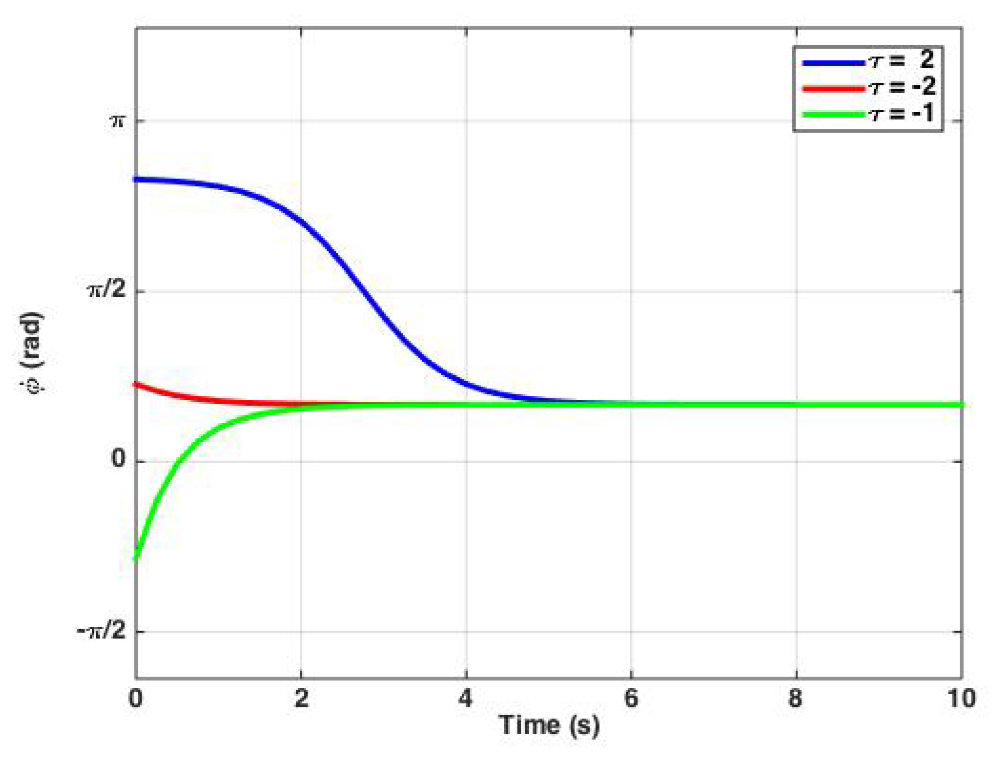
Starting with the canonical model (Equation (20)), we can decompose the system to find the dynamical descriptions of each oscillator’s amplitude and phase:

$$\dot{z_i}=A_1{z}_i+A_{21}{\left|z_i\right|}^2{z}_i+ϵ{\dot{z_i}}_c.$$

(21)

Considering the polar transformation of $z_i$: $z_i=r{e}^{i{\varphi }_i}$, represents the canonical model in polar coordinates. We provide all the algebraic calculations in Appendix C and the final coupled nonlinear differential equations that govern the dynamics of the amplitudes and phases are:

$$\begin{array}{cc}\hfill \dot{r_i}=& \alpha r_i+\beta r_i^3+\hfill \\ \hfill & ϵ[n_{1}cos({\varphi }_j-{\varphi }_i)+n_{2}cos({\varphi }_j+{\varphi }_i)]r_j\hfill \\ \hfill & +ϵ[n_{4}cos({\varphi }_j+{\varphi }_i)\hfill \\ \hfill & +n_{3}cos({\varphi }_j-{\varphi }_i)+n_{5}cos({\varphi }_j-3{\varphi }_i)+n_{6}cos({\varphi }_j+3{\varphi }_i)]r_i^2{r}_j\hfill \\ \hfill & +ϵ[n_{7}cos({\varphi }_i+3{\varphi }_j)+n_{8}cos({\varphi }_j+{\varphi }_i)]r_j^3\hfill \end{array}$$

(22)

and

$$\begin{array}{cc}\hfill \dot{{\varphi }_i}=& \omega +\delta r_i^2\hfill \\ \hfill & +ϵ[l_{1}sin({\varphi }_j-{\varphi }_i)+l_{2}sin({\varphi }_j+{\varphi }_i)]\frac{r_j}{r_i}\hfill \\ \hfill & +ϵ[l_{4}sin({\varphi }_j+{\varphi }_i)\hfill \\ \hfill & +l_{3}sin({\varphi }_j-{\varphi }_i)+l_{5}sin({\varphi }_j-3{\varphi }_i)+l_{6}sin({\varphi }_j+3{\varphi }_i)]r_i{r}_j\hfill \\ \hfill & +ϵ[l_{7}sin({\varphi }_i+3{\varphi }_j)+l_{8}sin({\varphi }_j+{\varphi }_i)]\frac{r_j^3}{r_i},\hfill \end{array}$$

(23)

where $i\ne j$ and $\delta$ is the imaginary part of constant $A_{21}$. We can derive relationships for the relative amplitude and phase of the two oscillators by defining $\varphi \left(t\right)={\varphi }_1\left(t\right)-{\varphi }_2\left(t\right)$ and $r\left(t\right)=r_1\left(t\right)-r_2\left(t\right)$ as relative phase and amplitude, respectively. We start with $\dot{r}=\dot{r_1}-\dot{r_2}$ and then substitute for $r_1$ and $r_2$ obtained in Equation (22). We do the same for the relative phase equation: $\dot{\varphi }=\dot{{\varphi }_1}-\dot{{\varphi }_2}$ using Equation (23).

In the special case of $r_1=r_2$ the relative amplitude dynamics is described by:

$$\dot{r}=ϵn_5(cos({\varphi }_2-3{\varphi }_1)-cos({\varphi }_1-3{\varphi }_2))r^3,$$

(24)

where the value of $n_5$ is given in Appendix C. Solutions of Equation (24) are shown in Figure 2 for different values of the bifurcation parameter $\alpha$.

By setting Equation (24) equal to zero, we found the fixed points, which are either $r^{*}=0$ or ${\varphi }^{*}=0,\pi$. We demonstrate the solutions of $\varphi$ for different values of the bifurcation parameter $\alpha$ in Figure 3.

3. Results

This section contains the main results of this paper. Here, we suggest an analytical solution of Equation (20) using approximating methods. In practice we were interested to find the relative phase dynamics of the two coupled canonical oscillators described above. We considered the compact format of Equation (20):

$$\dot{z_k}-A_1{z}_k-A_{21}{\left|z_k\right|}^2{z}_k=ϵ{\dot{z_k}}_c,$$

(25)

which describes the time evolution of two coupled canonical oscillators $(k=1,2)$. Finding the analytical solutions for z is not straight forward. To address this issue, we utilize the ansatz:

$$z_k\left(t\right)=c_k\left(t\right)e^{i{\omega }_{k}t}+{\overline{c}}_k\left(t\right)e^{-i{\omega }_{k}t}$$

(26)

as an approximate solution of this behavior with $c_k\left(t\right)=r_k{e}^{i{\varphi }_k\left(t\right)}$ as the time dependent amplitude of oscillations. ${\varphi }_k$ and ${\omega }_k$ are the phase and frequency of the oscillations of each oscillator, respectively. This approximate solution is true under the assumptions of slowly varying amplitude and rotating wave approximations; i.e., the time scale of their dynamics is much larger than $1/{\omega }_k$ ($\dot{c_k}\ll {\omega }_k$), and frequencies bigger than ${\omega }_k$ are neglected [1,9,14]. Differentiating this solution with respect to time yields:

$$\begin{array}{cc}\hfill \dot{z_k}\left(t\right)=& {\dot{c}}_k\left(t\right)e^{i{\omega }_k\left(t\right)}+\dot{c_k}{\left(t\right)}^{*}{e}^{-i{\omega }_k\left(t\right)}\hfill \\ \hfill & +i{\omega }_k{c}_k\left(t\right)e^{i{\omega }_k\left(t\right)}-i{\omega }_k{c}_k{\left(t\right)}^{*}{e}^{-i{\omega }_k\left(t\right)}.\hfill \end{array}$$

(27)

Knowing that:

$${\dot{c}}_k\left(t\right)={\dot{r}}_k{e}^{{i\varphi }_k\left(t\right)}+i{r}_k{\dot{\varphi }}_k\left(t\right)e^{{i\varphi }_k\left(t\right)}=({\dot{r}}_k+i{r}_k{\dot{\varphi }}_k\left(t\right))e^{i{\varphi }_k\left(t\right)},$$

(28)

Equation (27) becomes:

$$\begin{array}{cc}\hfill \dot{z_k}\left(t\right)=& ({\dot{r}}_k+i{r}_k{\dot{\varphi }}_k\left(t\right))e^{{i\varphi }_k\left(t\right)}{e}^{i{\omega }_k\left(t\right)}\hfill \\ \hfill & +({\dot{r}}_k-i{r}_k{\dot{\varphi }}_k\left(t\right))e^{{-i\varphi }_k\left(t\right)}{e}^{-i{\omega }_k\left(t\right)}\hfill \\ \hfill & +i{\omega }_k{r}_k{e}^{i{\varphi }_k\left(t\right)}{e}^{i{\omega }_k\left(t\right)}-i{\omega }_k{r}_k{e}^{{-i\varphi }_k\left(t\right)}{e}^{-i{\omega }_k\left(t\right)}.\hfill \end{array}$$

(29)

Without loss of generality, we assume equal amplitude for both oscillators, which means $r_1=r_2=r$. Note that even if the amplitudes are not equal, the relative phase dynamics do not get changed since we are analyzing the system under the assumption of slowly varying amplitude approximation; i.e., $\dot{r}\left(t\right)\ll \omega$. We note here the equations for the first canonical oscillator; the equations for the second oscillator are the same by switching the subindices. The left-hand side of Equation (25) after multiplying by $e^{-i{\varphi }_1}{e}^{-i{\omega }_1\left(t\right)}$ and regrouping is:

$$\begin{array}{cc}\hfill L.H.S\times e^{-i{\varphi }_1}{e}^{-i{\omega }_1\left(t\right)}=& (\dot{r}+ir\dot{{\varphi }_1}+i{\omega }_{1}r)(1-e^{-2i({\varphi }_1+{\omega }_1(t))})\hfill \\ & -((A_1+A_2)r-A{r}^3{(e^{i({\varphi }_1+{\omega }_1(t))}+e^{-i({\varphi }_1+{\omega }_1\left(t\right))})}^2)(1+e^{-2i({\varphi }_1+{\omega }_1\left(t\right))}).\hfill \end{array}$$

(30)

Equation (30) contains both oscillatory terms (exponential functions) with integer multiples of ${\omega }_1$ as the frequency and non-oscillating terms that do not contain these exponentials. By integrating over a time period given by $T=\frac{2\pi }{{\omega }_1}$ (averaging), all oscillatory terms vanish and only the non-oscillating terms remain:

$$L.H.S=\dot{r}+ir(\dot{{\varphi }_1}+{\omega }_1)-(A_1+A_2)r$$

(31)

We consider the right-hand side of Equation (25) and set $ϵ=1$ for now to ease the calculations. Recollecting the coupling terms on the $R.H.S.$ yields:

$$\begin{array}{cc}\hfill R.H.S.=& (B_1+B_2)r[e^{i({\varphi }_2+{\omega }_1\left(t\right))}+e^{-i({\varphi }_2+{\omega }_1\left(t\right))}]\hfill \\ \hfill & +(B_3+B_4+B_5+B_6+B_7+B_8-{\kappa }_1(B_1+B_2)\hfill \\ \hfill & -2{\kappa }_1(\overline{B_1}+\overline{B_2}))\times {[e^{i({\varphi }_1+{\omega }_1\left(t\right))}+e^{-i({\varphi }_1+{\omega }_1\left(t\right))}]}^2\hfill \\ \hfill & \times [e^{i({\varphi }_2+{\omega }_1\left(t\right))}+e^{-i({\varphi }_2+{\omega }_1\left(t\right))}]\hfill \\ \hfill & +(B_1{\kappa }_2+B_2\overline{{\kappa }_2})r^3{[e^{i({\varphi }_2+{\omega }_1\left(t\right))}+e^{-i({\varphi }_2+{\omega }_1\left(t\right))}]}^3.\hfill \end{array}$$

(32)

Introducing new coefficients as:

$$\left\{\begin{array}{c}M=B_1+B_2\hfill \\ N=B_3+B_4+B_5+B_6+B_7+B_8-{\kappa }_{1}M-2{\kappa }_1\overline{M}\hfill \\ P=B_1{\kappa }_2+B_2\overline{{\kappa }_2}\hfill \end{array}\right.$$

and substituting into the $R.H.S.$ gives:

$$\begin{array}{cc}\hfill R.H.S.=& Mr[e^{i({\varphi }_2+{\omega }_1\left(t\right))}+e^{-i({\varphi }_2+{\omega }_1\left(t\right))}]\hfill \\ \hfill & +N{r}^2{[e^{i({\varphi }_1+{\omega }_1\left(t\right))}+e^{-i({\varphi }_1+{\omega }_1\left(t\right))}]}^2\hfill \\ \hfill & \times [e^{i({\varphi }_2+{\omega }_1\left(t\right))}+e^{-i({\varphi }_2+{\omega }_1\left(t\right))}]\hfill \\ \hfill & +P{r}^3{[e^{i({\varphi }_2+{\omega }_1\left(t\right))}+e^{-i({\varphi }_2+{\omega }_1\left(t\right))}]}^3.\hfill \end{array}$$

(33)

Multiplying the R.H.S. by $e^{-i({\varphi }_1+{\omega }_{1}t)}$ gives:

$$\begin{array}{cc}\hfill R.H.S.=& Mr[e^{\left(i({\varphi }_2-{\varphi }_1)\right)}+e^{-i({\varphi }_2+{\omega }_1\left(t\right))}{e}^{-i({\varphi }_1+{\omega }_1\left(t\right))}]\hfill \\ \hfill & +N{r}^3{[e^{i({\varphi }_1+{\omega }_1\left(t\right))}+e^{-i({\varphi }_1+{\omega }_1\left(t\right))}]}^2\hfill \\ \hfill & \times [e^{i({\varphi }_2-{\varphi }_1)}+e^{-i({\varphi }_2+{\varphi }_1+2{\omega }_{1}t)}]\hfill \\ \hfill & +P{r}^3[e^{i({\varphi }_2-{\varphi }_1)}+e^{-i({\varphi }_2+{\varphi }_1+2{\omega }_{1}t)}].\hfill \end{array}$$

(34)

By averaging, only the first term survives and if we consider $ϵ$ not necessarily equal to 1:

$$R.H.S.=Mϵr{e}^{i({\varphi }_2-{\varphi }_1)}=Mϵr{e}^{i\varphi }$$

(35)

Now by equating the L.H.S. with the R.H.S. and including the second oscillator by letting $1\to 2$ and consequently $\varphi \to -\varphi$, we obtain:

$$\left\{\begin{array}{c}\dot{r}+ir(\dot{{\varphi }_1}+{\omega }_1)-(A_1+A_2)=Mϵr{e}^{i\varphi }\hfill \\ \dot{r}+ir(\dot{{\varphi }_2}+{\omega }_2)-(A_1+A_2)=Mϵr{e}^{-i\varphi }\hfill \end{array}\right.$$

(36)

Subtracting second equation from the first one gives:

$$ir(\dot{{\varphi }_1}-\dot{{\varphi }_2}+{\omega }_1-{\omega }_2)=Mϵr[e^{i\varphi }-e^{-i\varphi }].$$

(37)

By defining the relative frequency as $\omega ={\omega }_1-{\omega }_2$ and recalling that $sin\varphi =\frac{e^{i\varphi }-e^{-i\varphi }}{2i}$:

$$-ir(\dot{\varphi }-\omega )=Mϵr(2isin\varphi ).$$

(38)

Hence, the average relative phase dynamics is given by:

$$\dot{\varphi }=\omega -Csin\varphi .$$

(39)

where $C=2Mϵ$ is the total coupling coefficient and a complex number, due to M. We can reinterpret M and consequently C in terms of the initial Wilson–Cowan model parameters (refer to Appendix B):

$$M=B_1+B_2=c_1+i{c}_3,$$

(40)

so:

$$C=2Mϵ=2ϵ(c_1+i{c}_3).$$

(41)

Note that the magnitude of the total coupling coefficient is:

$$\left|C\right|=2ϵ\sqrt{c_1^2+c_3^2}.$$

(42)

It can be described as the coupling strength of the two canonical oscillators. This enables us to access a coupling coefficient based on the coefficients in the original Wilson-Cowan model. As one can see, the value of C is independent of $c_2$ and $c_4$. This means that the average phase dynamics of the system do not depend on $c_2$ and $c_4$ coefficients. C being a complex number indicates the rotation of the two canonical oscillators in phase space or a delay between their relative oscillations. Integrating Equation (39) gives us more insights:

$$t=\int \frac{d\varphi }{\omega -Csin\varphi }$$

(43)

There is a pole at $\varphi =si{n}^{-1}\left(\frac{\omega }{C}\right)$. This is the fixed point of the system that gives the steady-state solution of the relative phase. We will confirm it later by taking the limit of $\varphi$ as time tends to infinity. In other words:

$${\varphi }^{*}={sin}^{-1}\left(\frac{\omega }{C}\right).$$

(44)

Equation (44) gives us the constraint of having convergent solutions; i.e.:

$$|\frac{\omega }{C}|\le 1.$$

(45)

This is the convergence interval in which we evaluate the integral of Equation (43). Before solving this integral we consider the special case when the two oscillators have the same frequency, i.e., $\omega =0$, such that the integration process becomes simpler:

$$-Ct=\int \frac{d\varphi }{sin\varphi }=\frac{1}{2}ln(tan\frac{\varphi }{2})+c,$$

(46)

where c is the constant of integration and depends on the initial conditions. We solve this equation for $\varphi$:

$$ln(tan\frac{\varphi }{2})=-2(Ct+c)⟹tan\frac{\varphi }{2}=exp(-2(Ct+c));$$

(47)

hence, the relative phase is:

$$\varphi =2{tan}^{-1}(e^{-2(Ct+c)}).$$

(48)

This result can be written in terms of the integration time interval $\tau =\frac{c}{C}$:

$$\varphi =2{tan}^{-1}\left(e^{-2C(t-\tau )}\right).$$

(49)

Some plots of the relative phase are shown in Figure 4 for different initial conditions.

In the general case of Equation (43) in which the canonical oscillators do not necessarily have the same frequency, i.e., $\omega \ne 0$, the solution within the convergence region ($|\frac{\omega }{C}|\le 1$) is given by either:

$$t=-{\displaystyle \frac{2}{\sqrt{C^2-{\omega }^2}}}{tanh}^{-1}({\displaystyle \frac{\omega tan\frac{\varphi }{2}-C}{\sqrt{C^2-{\omega }^2}}})+c$$

(50)

or:

$$t=-{\displaystyle \frac{2}{\sqrt{C^2-{\omega }^2}}}{coth}^{-1}({\displaystyle \frac{\omega tan\frac{\varphi }{2}-C}{\sqrt{C^2-{\omega }^2}}})+c,$$

(51)

depending on the initial conditions ${\varphi }_1\left(0\right)$ and ${\varphi }_2\left(0\right)$.

Hence, the average relative phase is given by:

$$\varphi =2{tan}^{-1}\{{\displaystyle \frac{\sqrt{C^2-{\omega }^2}}{\omega }}tanh({\displaystyle \frac{-\sqrt{C^2-{\omega }^2}(t-c)}{2}})+\frac{C}{\omega }\}$$

(52)

or:

$$\varphi =2{tan}^{-1}\{{\displaystyle \frac{\sqrt{C^2-{\omega }^2}}{\omega }}coth({\displaystyle \frac{-\sqrt{C^2-{\omega }^2}(t-c)}{2}})+\frac{C}{\omega }\}.$$

(53)

In either case, taking the limit of this average relative phase as time tends to infinity gives us:

$$\underset{t\to \infty }{lim}\varphi =2{tan}^{-1}\{{\displaystyle \frac{C-\sqrt{C^2-{\omega }^2}}{\omega }}\}.$$

(54)

This angle is the fixed-point or the steady-state solution that we have already mentioned (Equation (44)). As a proof, recall that

$$sin2x=2sinxcosx=2tanx{cos}^{2}x={\displaystyle \frac{2tanx}{1+{tan}^{2}x}}$$

and if we set $x=\frac{{\varphi }^{*}}{2}$, then:

$$sin{\varphi }^{*}={\displaystyle \frac{2({\displaystyle \frac{C-\sqrt{C^2-{\omega }^2}}{\omega }})}{1+{({\displaystyle \frac{C-\sqrt{C^2-{\omega }^2}}{\omega }})}^2}}=\frac{\omega }{C}\Rightarrow {\varphi }^{*}={sin}^{-1}(\frac{\omega }{C}).$$

(55)

In Figure 5 we illustrate some solutions of the relative phase for some different initial conditions.

The convergence of the average relative phase of the two canonical oscillators to a fixed point is an indicator of phase-locking. After some amount of time that depends on their initial conditions, the two oscillators become phase-locked; i.e., they tend to oscillate with a fixed relative phase.

4. Discussion

The canonical model that we studied in this paper is the normal form of the Wilson–Cowan oscillators about a Hopf bifurcation point. The Hopf bifurcation in dynamical systems particularly refers to the development of periodic orbits from an equilibrium or a stable fixed point as an order parameter crosses a critical value [15]—in this paper the bifurcation parameter $\alpha$ (refer to Equations (13), (22) and (23)). This is a point of interest in auditory neuroscience, for example, in modeling approaches that have the potential to link neural dynamics to sound perception [16,17]. Other physical examples include the identification of stable oscillations in nonlinear waves [15]. Nevertheless, if another type of bifurcation is of interest, the normal form could be modified to resemble that particular type of bifurcation. This is because of the fact that normal forms are generic and enable us to remove the nonlinear terms that are not necessary going to be present for our specific purpose.

This work provided both an overview and detailed analysis of the coupled canonical oscillators of Wilson–Cowan-type neural field models, along with a novel methodology to check the interesting solutions. As a recapitulation of previous studies in the literature, we re-derived the canonical models of single and two coupled Wilson–Cowan oscillators under no external stimulus, Equations (13) and (20), respectively. As described in the Methods section, we utilized two theorems in nonlinear dynamical systems that give us constraints on the order of transformations during Hopf bifurcation to find the most compact form of the canonical model. The evolutions of amplitude and phase of each oscillator were found by representing the canonical model in the polar coordinates, Equations (22)–(24), and the solutions were plotted in time for different values of the bifurcation parameter, $\alpha$, along with the calculation of the fixed points. The damped, critical and spontaneous behaviors were seen as the values of $\alpha$ changes from −1 to 0 and then to 1, respectively (see Figure 2 and Figure 3). These were compatible with the behavior of the coupled oscillators at the Hopf bifurcation, as expected. By integrating knowledge and understanding from the basic mathematics and nonlinear dynamics along with our biophysical understanding of the brain, we presented solutions for the entrainment of two coupled canonical oscillators, which are analyzed in the Results section. These solutions are in line with our previous understanding of coupled nonlinear oscillators; however, a more straightforward method is presented using slowly varying amplitude and rotating wave approximations that helps us obtain approximate analytical solutions of the average relative phases of the two coupled oscillators. The time evolution of the average relative phase is given by Equation (49) for an special case wherein the frequencies of the two oscillators are equal. However, we were able to analytically calculate the average relative phase dynamics in a more general regime wherein the frequencies of the two oscillators were not necessarily equal; see Equations (52) and (53). The results were plotted in Figure 4 and Figure 5 for some different values of the initial conditions. The steady-state of the system, the fixed relative phases of the oscillators are given by Equation (55). The main novel aspect of the proposed method is that it enables investigators to directly relate the parameters in the canonical model to the original oscillatory population model of Wilson–Cowan; for example, see Equation (42). On the other hand, using the ansatz in Equation (26) we overcame the cumbersome task of solving the dynamics of the coupled canonical oscillators that traditionally have been addressed by the method of averaging [15].

Bifurcation analysis and dynamical properties of the canonical model, including phase planes, were investigated in detail in a more general regime of forced canonical oscillators [4] and due to their extensivity, were not presented in this study. The effects of the nonlinear terms in the canonical model, specifically on the resonance patterns, were analyzed and compared with the Wilson–Cowan model in an analytical and simulation study [3], and the analysis of higher order nonlinear terms was out of the scope of this paper.

We considered some assumptions in our analysis to ease the calculations. In all of the study, we considered no external stimulus present in the system. Traditionally, external inputs could be considered within the sigmoidal functions’ arguments of the neural field model and consequently would be present in the Taylor expansions of those sigmoid functions. However, the external inputs could be simply considered as direct additive terms as in case of the canonical oscillator, which was investigated in detail in a previous study [4]. For the sake of simplicity, we considered the coupled canonical oscillators to be identical. Nevertheless, one can consider them non-identicall and obtain the same oscillatory terms as in the canonical model but with different coefficients. The average relative phase calculations are done under the assumption of small perturbations; i.e., the time evolution of the canonical oscillators’ amplitudes are much smaller than their relative frequency. If we are in a regime in which this assumption is not true anymore, the average relative phases of the two canonical oscillators still could be found numerically but not explicitly.

The results of this study contribute to applications such as neural network modelings that target desired or unwanted resonance in the oscillatory system under investigation. The methodology of deriving the single and coupled canonical models presented here could be generalized for any Wilson–Cowan-type activity rate model and any number of oscillators.

References

1. Fuchs, A. Nonlinear Dynamics in Complex Systems: Theory and Applications for the Life-, Neuro- and Natural Sciences; Springer: Berlin, Germany, 2013. [Google Scholar]
2. Izhikevich, E.M. Dynamical Systems in Neuroscience; The MIT Press: Cambridge, MA, USA, 2007. [Google Scholar]
3. Large, E.W.; Almonte, F.V.; Velasco, M.J. A canonical model for gradient frequency neural networks. Phys. D 2010, 239, 905–911. [Google Scholar] [CrossRef]
4. Kim, J.C.; Large, E.W. Signal Processing in Periodically Forced Gradient Frequency Neural Networks. Front. Comput. Neurosci. 2015, 9, 152. [Google Scholar] [CrossRef] [PubMed] [Green Version]
5. Duke, T.; Andor, D.; Julicher, F. Physical Basis of Interference Effects in Hearing. Ann. Henri Poincaré 2003, 4, 667–669. [Google Scholar] [CrossRef]
6. He, J.H. Homotopy perturbation method for bifurcation of nonlinear problems. Int. J. Nonlinear Sci. Numer. Simul. 2005, 6, 207–208. [Google Scholar] [CrossRef]
7. Bayat, M.; Pakar, I.; Emadi, A. Vibration of electrostatically actuated microbeam by means of homotopy perturbation method. Struct. Eng. Mech. 2013, 48, 823–831. [Google Scholar] [CrossRef]
8. Bayat, M.; Pakar, I.; Domairry, G. Recent developments of some asymptotic methods and their applications for nonlinear vibration equations in engineering problems: A review. Lat. Am. J. Solids Struct. 2012, 9, 1–93. [Google Scholar] [CrossRef] [Green Version]
9. Bogoliubov, N.N.; Mitropolsky, Y.A. Asymptotic Methods in the Theory of Nonlinear Oscillators; Hindustan Publishing Corporation: Delhi, India, 1961. [Google Scholar]
10. Wiggins, S. Introduction to Applied Nonlinear Dynamical Systems and Chaos; Text in Applied Mathematics; Springer: Berlin, Germany, 2003; Volume 2. [Google Scholar]
11. Yu, P. Computation of the simplest normal forms with perturbation parameters based on Lie transformation and rescaling. J. Comput. Appl. Math. 2002, 144, 359–373. [Google Scholar] [CrossRef] [Green Version]
12. Wilson, H.R.; Cowan, J.D. Excitatory and Inhibitory Interactions in Localized Populations of Modeled Neurons. Biophys. J. 1972, 12, 1–24. [Google Scholar] [CrossRef] [Green Version]
13. Hoppensteadt, F.C.; Izhikevich, E.M. Weakly Connected Neural Networks; Appied Mathematical Sciences; Springer: Berlin, Germany, 1997; Volume 126. [Google Scholar]
14. Fuchs, A.; Jirsa, V.K.; Haken, H.; Kelso, J.A. Scott Extending the HKB model of coordinated movement to oscillators with different eigenfrequencies. Biol. Cybern. 1996, 74, 21–30. [Google Scholar] [CrossRef]
15. Marsden, J.E.; McCracken, M. The Hopf Bifurcation and Its Applications; Applied Mathematical Sciences; Springer: Berlin, Germany, 1976; Volume 19. [Google Scholar]
16. Lerud, K.D.; Almonte, F.V.; Kim, J.C.; Large, E.W. Mode-locking neurodynamics predict human auditory brainstem responses to musical intervals. Hear. Res. 2014, 308, 41–49. [Google Scholar] [CrossRef] [PubMed]
17. Farokhniaee, A.A. Simulation and Analysis of Gradient Frequency Neural Networks. Ph.D. Thesis, University of Connecticut Graduate School, Mansfield, CT, USA, 2016. [Google Scholar]
Figure 1. The nullclines. Nullclines of both Wilson–Cowan (black) and canonical (blue) models. Here a = 1 , b = c = ω = 1.7 , d = 1 , α = 0 , β = 0.75 .
Mathematics 08 01312 g001
Figure 2. The solutions of r for different values of the bifurcation parameter α . These solutions exhibit different behaviors of the coupled oscillators, as we changed the bifurcation parameter α . For α = 1 < 0 we have damped oscillations, and for α = 0 we faced critical ones. For α = 1 spontaneous oscillation was the result. In this figure a = α + 1 , b = c = ω = 5 , d = a 2 , ϵ = 0.1 , c 1 = c 2 = c 3 = c 4 = ϵ , β = A 21 and δ = 0.1 . The initial conditions were r 1 = r 2 = 1 , ϕ 1 = π and ϕ 2 = π / 6 .
Mathematics 08 01312 g002
Figure 3. The solutions of ϕ for different values of the bifurcation parameter α . For the two cases of α < 0 (damped) and α = 0 (critical) the two oscillators become in-phase with the relative phase of ϕ = 0 . Obviously, the rate of change of ϕ for the damped oscillation is greater than the critical one. When α > 0 (spontaneous), the two oscillators become anti-phase. In this figure a = α + 1 , b = c = ω = 10 , d = a 2 , ϵ = 0.1 , c 1 = c 2 = c 3 = c 4 = ϵ , β = A 21 and δ = 0.1 . The initial conditions were r 1 = r 2 = 1 , ϕ 1 = π and ϕ 2 = π / 6 .
Mathematics 08 01312 g003
Figure 4. The evolution of relative phase when ω 1 = ω 2 . The relative phase ( ϕ ) as a function of time for different initial conditions when C = 0.02 . This is a special case when the relative frequency of the oscillators ω is zero, which means they oscillate with the same frequency. One can see that they become phase-locked as time increases. In this special case, since ω = 0 , the fixed relative phase will be π .
Mathematics 08 01312 g004
Figure 5. The evolution of relative phase when ω 1 ω 2 . The relative phase ( ϕ ) is a function of time for different initial conditions while C = 2 and ω = 1 , so we can see the convergence of the solutions and phase-locking phenomenon. In this special case, since ω = 1 and C = 2 , the fixed relative phase will be π 6 .
Mathematics 08 01312 g005