Towards a Better Basis Search through a Surrogate Model-Based Epistasis Minimization for Pseudo-Boolean Optimization

Abstract

Epistasis, which indicates the difficulty of a problem, can be used to evaluate the basis of the space in which the problem lies. However, calculating epistasis may be challenging as it requires all solutions to be searched. In this study, a method for constructing a surrogate model, based on deep neural networks, that estimates epistasis is proposed for basis evaluation. The proposed method is applied to the Variant-OneMax problem and the $NK$-landscape problem. The method is able to make successful estimations on a similar level to basis evaluation based on actual epistasis, while significantly reducing the computation time. In addition, when compared to the epistasis-based basis evaluation, the proposed method is found to be more efficient.

1. Introduction

In terms of computation, various challenges such as black-box problems still exist. Multiple attempts have been made to resolve the difficulties by constructing surrogate models based on deep learning [1,2].

When we use a basis other than the standard basis, the structure of problem space can be quite different from the original one. Mbarek et al. [3,4] changed the standard basis of a vector space to ensure the efficient performance of an algorithm. Seo et al. [5] modified problem space by nontrivial encoding through a method changing the standard basis. The effects of basis change on a genetic algorithm (GA) in binary encoding have been investigated [6]. Furthermore, it has been shown that using this method, problem space can be fundamentally changed in graph problems, the performance of GAs gets affected. There were several studies that measured the problem difficulty from the view of epistasis [7,8]. To search a basis to smooth the ruggedness of the problem space, Lee and Kim [9,10] proposed a method that used a meta-GA and an epistasis-based basis evaluation method which largely reduced computational time over the meta-GA. In order to calculate epistasis accurately, all feasible solutions need to be first searched. However, searching all solutions becomes challenging as the complexity of the problem increases. They have resolved this issue by estimating the epistasis of solution samples.

However, estimating the epistasis using samples of the solutions still requires a large computational cost. Therefore, in this study, deep neural networks (DNNs) are used to construct an epistasis-estimating surrogate model to remarkably reduce the computational cost.

The remaining of the paper is consisted as follows. The background is explained in Section 2. In Section 3, related studies are introduced. First, a method of smoothing the ruggedness of the problem space using a meta-GA is described, and then, a study related to basis evaluation based on actual epistasis is described. Section 4 discusses the deep learning-based epistasis estimation method proposed in this study. In Section 5, the results of applying the basis change to a GA are analyzed. We draw conclusions in Section 6.

2. Backgrounds and Test Problems

In this section, we describe various backgrounds needed to understand the rest of this paper. In Section 2.1 and Section 2.2, we describe basis and epistasis, respectively. We explain how we calculated epistasis in Section 2.3. Section 2.4 and Section 2.5 discuss the deep learning and surrogate models, respectively. In Section 2.6, we introduce test problems used in our experiments.

2.1. Basis

In linear algebra, the basis of a vector space is the linear independent vectors that span the vector space [11,12]. In other words, they are vectors that give a unique representation as a linear combination to any vector in the vector space. The basis can be defined as follows:

Definition 1.

[Basis] Basis B, which is a basis of V, which is a vector space, over $\mathbb{F}$, which is a field, is a linear independent subset of V that spans V. Satisfying the following two conditions means that B, which is a subset of V, is a basis:

• Linear independence property: for every finite subset $\{b_1,b_2,\dots ,b_n\}$ of B and every $a_1,a_2,\dots ,a_n$ in $\mathbb{F}$, if $a_1{b}_1+a_2{b}_2+\cdots +a_n{b}_n=0$, then necessarily $a_1=a_2=\cdots =a_n=0;$
• Spanning property: it is possible to choose $v_1,v_2,\dots ,v_n$ in $\mathbb{F}$ and $b_1,b_2,\dots ,b_n$ in B such that $v=v_1{b}_1+v_2{b}_2+\cdots +v_n{b}_n$ for every vector v in V.

The standard basis for vector space ${\mathbb{Z}}^n$ is $e_1,e_2,\dots ,e_n$, where $e_i$ is a column vector with the i-th component of 1 and remaining components of 0 If the basis is expressed as a 0-1 matrix, it becomes the identity matrix. Changing the identity matrix into an invertible one can lead to the transformation of the standard basis.

$$B_S=\left\{e_1,e_2,\dots ,e_n\right\}=\left\{\left(\begin{array}{c}1\\ 0\\ ⋮\\ 0\end{array}\right)\left(\begin{array}{c}0\\ 1\\ ⋮\\ 0\end{array}\right)\cdots \left(\begin{array}{c}0\\ 0\\ ⋮\\ 1\end{array}\right)\right\}\iff \left(\begin{array}{cccc}1& 0& \cdots & 0\\ 0& 1& \cdots & 0\\ ⋮& ⋮& \ddots & ⋮\\ 0& 0& \cdots & 1\end{array}\right)=I_n$$

(1)

2.2. Epistasis

In GAs, epistasis refers to any type of gene interaction. A more complex gene interaction implies more complex problems and greater epistasis. On the other hand, if the gene interaction is independent, the epistasis becomes zero.

A method proposed by Lee and Kim [10] used the epistasis proposed by Davidor [13]. Equations for calculating the epistasis are provided in Section 2.3.

Typically, the standard basis is used in binary encoding. When the evaluation functions in the standard basis with complex interdependencies of basis vectors are changed to another basis, with the aim of smoothing the ruggedness of the problem space, the calculation of the evaluation functions becomes simpler and the epistasis decreases as well. However, as all the feasible solutions need to be searched first to calculate the epistasis, the epistasis of the sampled solutions was calculated in [10] and, based on this, an estimation was made for the actual epistasis.

2.3. How to Calculate Epistasis

In this paper, we used the formula proposed by Davidor [13] to calculate epistasis. Equations for calculating epistasis in Section 2.2 as follows. A string S is composed of l elements $(s_1,s_2,\dots ,s_l)$, where $s_i\in \{0,1\}$ for each $i=1,2,\dots ,l$.

The $GrandPopulation\mathrm{\Gamma }$ is the group of all strings of length l,

$$\mathrm{\Gamma }=\prod _{i=1}^l\{0,1\}$$

(2)

Let $Pop$ denote a sample of $\mathrm{\Gamma }$, where the sample is selected uniformly and with replacement. $N_{Pop}$ is the size of the sample $Pop$. $v\left(S\right)$ is the fitness of a string S.

The average fitness value of $Pop$ is:

$$V=\frac{1}{N_{Pop}}\sum _{S\in Pop}v\left(S\right)$$

(3)

The number of string S in $Pop$ that match $s_i=a$ is denoted by $N_i\left(a\right)$. If ${Pop}_{S_i=a}$ is the set of all strings in $Pop$ with the allele a in their i-th position. The average allele value $A_i\left(a\right)$ is denoted by

$$A_i\left(a\right)=\frac{1}{N_i\left(a\right)}\sum _{S\in {Pop}_{S_i=a}}v\left(S\right)$$

(4)

The excess allele value $X_i\left(a\right)$ is defined by:

$$X_i\left(a\right)=A_i\left(a\right)-V$$

(5)

The excess genic value $X\left(S\right)$ is:

$$X\left(S\right)=\sum _{i=1}^l{X}_i\left(S_i\right)$$

(6)

The genic value $A\left(S\right)$ of a string S is defined as:

$$A\left(S\right)=X\left(S\right)+V$$

(7)

Finally, the epistasis variance $\epsilon$(S) is:

$$\epsilon \left(S\right)={\left\{v\right(S)-A(S\left)\right\}}^2$$

(8)

2.4. Deep Learning

Deep learning [14] is a high-level abstraction method that uses a combination of various non-linear techniques. This technology is currently being used in various domains of the modern society. In particular, it has brought significant developments in fields like computer vision, speech recognition, and natural language processing.

A deep neural network (DNN) is one kind of artificial neural network (ANN) that consists of various hidden layers between the input layer and output layer. Regardless of the linearity, a DNN can model complex relationships that change from the input to the output. In addition, there are various ANN models such as convolutional neural network (CNN) [15], recurrent neural network [16], and restricted Boltzmann machine [17].

2.5. Surrogate Model

Surrogate model is a model used to replace tasks such as those of complex and time-consuming calculations [18]. There are several real-world simulations that are extremely time-consuming or difficult to implement in a realistic manner. These simulations may take days or even weeks to produce the results. As these tasks are highly time intensive, performing simulations in many cases is almost infeasible. In such cases, surrogate models are used for the simulations. Sreekanth and Datte [19] built a surrogate model for coastal aquifer management. Eason and Cremaschi [20] used an ANN-based surrogate model for a chemical simulation.

Surrogate models are also used in the fields of mathematics and optimization. Some studies have been conducted to optimize various objective functions using surrogate models [21,22,23,24,25,26]. Specifically, these studies attempted to optimize the cost-expensive black-box problems. In particular, several studies have proposed the use of Walsh-based surrogate models to reduce the computational cost associated with pseudo-Boolean problems [27,28,29].

Similarly, these models have been adopted to reduce computational costs in several other fields as well. Deep learning techniques can also be used to replace black-box evaluation. To this end, surrogate models using deep learning have been developed [2,30,31,32,33,34,35]. Deep learning can be a powerful method for estimating the evaluation values that are difficult to compute in a realistic manner. This study intends to reduce the computation time by constructing a DNN-based surrogate model that estimates the epistasis corresponding to a basis.

2.6. Test Problems

This study tested the same problems as those in the experiments conducted by Lee and Kim [10]. The OneMax problem is the maximization of the number of 1s in a binary vector. Variant-OneMax is defined as the problem that maximizes the number of 1s in the binary vectors that are changed from the standard basis to another basis. When $B_S$ is the standard basis and B is another basis, the change of $B_S$ to B can be expressed as an invertible matrix ${\left[T\right]}_{B_S}^B$. When we change the basis, a vector v can be represented as ${\left[T\right]}_{B_S}^{B}v={\left[v\right]}_B$. The fitness value of ${\left[v\right]}_B$ counts the number of 1s in ${\left[v\right]}_B$. The optimal solution to the Variant-OneMax problem is that all elements are 1.

The $NK$-landscape problem defined by Kauffman [36] comprises of chromosome S of length N, and each gene has a dependency on the other K numbers of genes. The fitness contribution $f_i$ of the gene at locus i depends on the allele $S_i$ and K other alleles $S_{i1},S_{i2},\dots ,S_{iK}$. The fitness f of a point $S=(S_1,S_2,\dots ,S_N)$ can then be expressed as follows:

$$f\left(S\right)=\frac{1}{N}\sum _{i=1}^N{f}_i(S_i,S_{i1},S_{i2},\dots ,S_{iK})$$

(9)

As the $NK$-landscape problem is an NP-complete problem, it is difficult to find the global optimum, and therefore, it is employed extensively in the optimization field [37]. Additionally, the level of difficulty of the problem can be adjusted through N, which represents the overall size of the landscape and K, which represents the number of its local hills and valleys. The higher K is, the more rugged the problem space is.

3. Prior Work on Searching Basis

In this section, we introduce prior work on searching basis. We describe the work of finding a good basis using a meta-GA and the GA combined with epistasis-based basis evaluation.

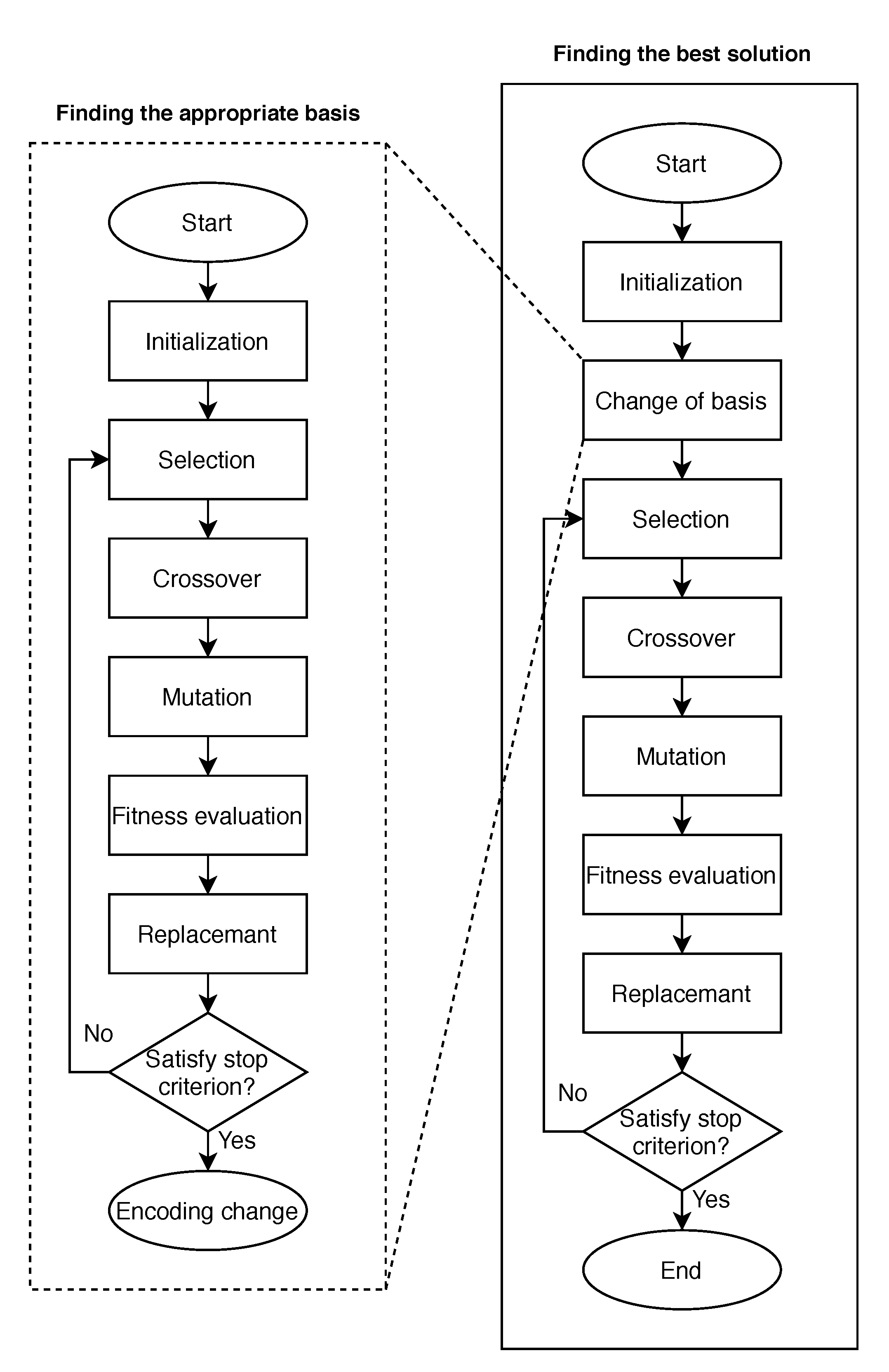
3.1. Basis Searching with a Meta-GA

A good basis can improve the performance of a GA. Lee and Kim [9] proposed a method of using a meta-GA to search a good basis.

The performance improvement was demonstrated for the $NK$-landscape problem by changing the standard basis to the other basis obtained using the meta-GA. However, the time complexity of searching the basis with their meta-GA was found to be $O\left(2^{n^2}\right)$. Hence, the method of obtaining a good basis using the meta-GA is not practical as it is extremely time-intensive.

3.2. Epistasis-based Basis Evaluation

Lee and Kim [10] proposed an epistasis-based basis evaluation method and subsequently applied the proposed method to a GA in order to search a good basis. They converted the complex problem into a simpler one by changing the basis.

Their epistasis-based basis evaluation method was conducted as follows. With a certain given basis, the sampled solution set S was obtained from the problem, following which $S^{\prime }$ was obtained by a basis change. The epistasis in $S^{\prime }$ was calculated. A low value of the epistasis represented the higher appropriateness of the basis for the problem. When the gene size was represented by l and the number of the sampled solution set S was represented by s, the time required for calculating the epistasis was $O\left(l^{2}s\right)$.

Next, GAs using the epistasis evaluation were described. A basis could be represented as an invertible matrix. If $E_i$s were elementary matrices, any invertible matrix T could be expressed as $T=E_1\times E_2\times \dots \times E_{m_T}$. Each basis was represented as a variable-length string encoding meaning the multiplication of the elementary matrices [38].

The parents were aligned according to the Wagner–Fischer algorithm [39], after which a uniform crossover operator was applied. For the selection operator, the tournament operator was applied to select the best solution out of three parents. The mutation operator was used by applying either insertion, deletion, or replacement. The replacement was applied by replacing the parent households with child households.

Experiments were conducted on the Variant-OneMax problem and the $NK$-landscape problem that are described in Section 2.6. After performing the GA, to identify another basis for each problem, the optimal solutions were found by searching solutions for each problem one hundred times, independently. This was conducted by changing to the basis found by the GA. Thereafter, the experimental results were compared for three cases: the case where the basis change was not conducted, the case where a meta-GA was applied, and the case where the epistasis-based basis evaluation method was used. The case with using the meta-GA showed better results overall. However, as the computation of the meta-GA is time intensive, it is difficult to use in practice. The epistasis-based basis evaluation method yielded better results compared to the basis with no change made, and required less time compared with the meta-GA. Thus, considering both the experimental results and process time, the epistasis-based basis evaluation method was shown to be the most efficient method. Further, the calculation of the epistasis before and after the basis change showed a decrease in the epistasis, thereby indicating the effectiveness of the presented model. However, this method was still time-consuming as it required calculating the epistasis for each solution in the solution set. We try to remarkably reduce the computational cost by estimating epistasis using deep learning.

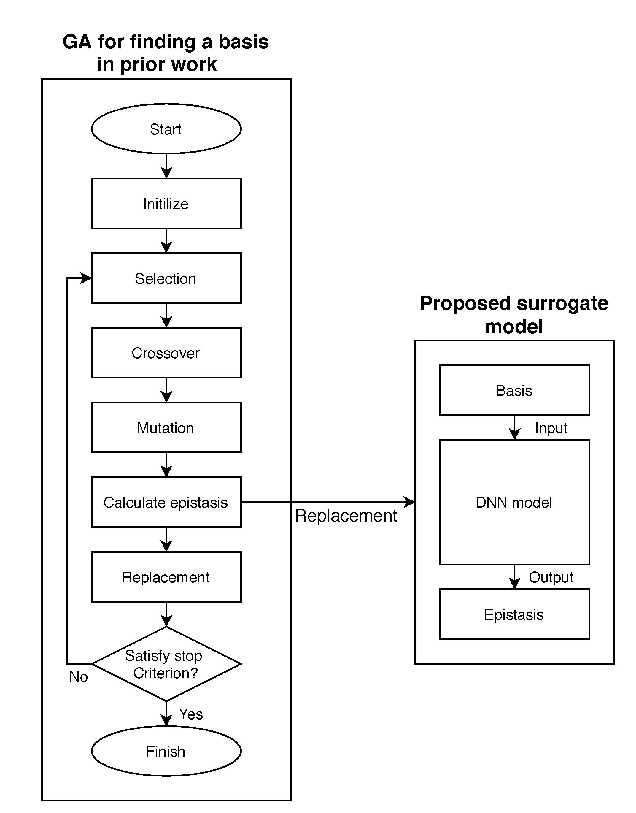
4. Proposed Method Based on Surrogate Model

In this section, we describe the proposed epistasis estimation method based on a surrogate model. We present how to estimate epistasis using deep learning in Section 4.1. In Section 4.2, we introduce our GA combined with the proposed surrogate model.

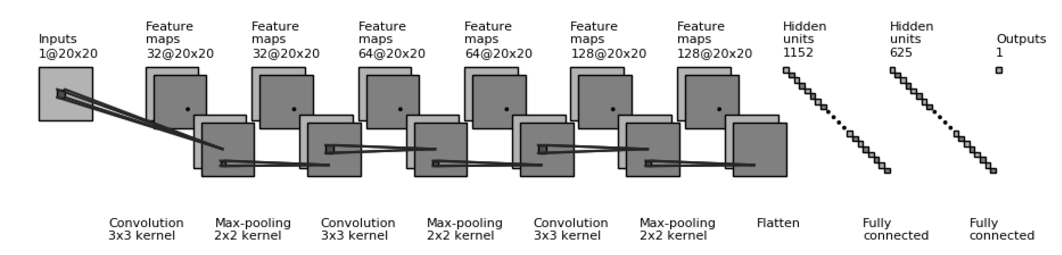
4.1. Surrogate Model-Based Epistasis Estimation Using Deep Learning

In Section 4.2, we confirmed that the complexity of a problem on a basis could be represented by an epistasis. This was done by estimating the actual epistasis using a sampled solution set as the problem of searching all the solutions to calculate the epistasis. However, as this estimated method of computing the epistasis was still time-consuming, we expected that deep learning could be used to further reduce the computation time.

We intended to apply a deep learning model when the basis and the estimated epistasis, in Section 4.2, were considered to be input and output, respectively. In practice, it is nearly impossible to search all the solutions to calculate epistasis. However, if the epistasis can be successfully estimated using a deep learning model, the deep learning model can be viewed as an objective function for estimating the epistasis. A surrogate model estimates an unknown objective function based on the accumulated input and output data. Therefore, the corresponding deep learning model can be considered to be a surrogate model.

Kim et al. [40] and Kim and Kim [41] introduced an epistasis estimation method using a DNN model. Experiments were conducted using DNN and CNN to determine the deep learning model that was more suitable for epistasis estimation. The hyperparameters for the DNN and CNN models are detailed in

Table 1. The hyperparameter configuration of deep neural network (DNN) and  convolutional neural network (CNN).

Hyperparameter	DNN Value	CNN Value
Learning rate	0.001	0.001
Epoch	1000	1000
Dropout rate	0.5	0.5
Loss function	RMSE	RMSE
Optimizer	“Adam”	“Adam”
Number of layers	5	N/A
Number of neurons per layer	$N^2/2$	N/A

* N: the dimension of each problem.

, and the used structure of the CNN model is shown in Figure 1.

The data used in our experiments were from the populations obtained by the GA experiments of Lee and Kim [10] for searching the basis on each problem. Further, 10-fold cross-validation was conducted after removing duplicated data within the dataset. The results of the experiment are summarized in

Table 2. Experimental results of epistasis estimation using DNN and CNN.

Problems		Deduplication		DNN				CNN
				Actual	Estimated	Ratio (%)	Time (s)	Actual	Estimated	Ratio (%)	Time (s)
		Before	After	Average	Average			Average	Average
Variant- OneMax	$N=20$	6400	1863	$4.06$	$4.03$	0.74	21.5	$4.06$	$4.03$	0.88	36.0
	$N=30$	14,400	2291	$4.44$	$4.40$	0.72	24.7	$4.44$	$4.41$	0.63	60.1
	$N=50$	40,000	9767	$8.72$	$8.74$	0.23	103.8	$8.72$	$8.75$	0.36	680.1
$NK$- landscape	$N=20$ $K=3$	6400	1403	$3.08\times {10}^{-3}$	$3.15\times {10}^{-3}$	2.26	18.8	$3.08\times {10}^{-3}$	$3.01\times {10}^{-3}$	2.32	31.5
	$N=20$ $K=5$	6400	1141	$3.16\times {10}^{-3}$	$3.18\times {10}^{-3}$	0.53	18.4	$3.16\times {10}^{-3}$	$3.22\times {10}^{-3}$	1.62	28.9
	$N=20$ $K=10$	6400	1527	$4.08\times {10}^{-3}$	$4.09\times {10}^{-3}$	0.09	18.4	$4.08\times {10}^{-3}$	$4.07\times {10}^{-3}$	0.43	32.5
	$N=30$ $K=3$	14,400	2124	$1.77\times {10}^{-3}$	$1.80\times {10}^{-3}$	1.51	22.0	$1.77\times {10}^{-3}$	$1.79\times {10}^{-3}$	1.17	58.9
	$N=30$ $K=5$	14,400	2822	$2.49\times {10}^{-3}$	$2.52\times {10}^{-3}$	1.01	23.9	$2.49\times {10}^{-3}$	$2.51\times {10}^{-3}$	0.71	72.2
	$N=30$ $K=10$	14,400	3609	$2.58\times {10}^{-3}$	$2.58\times {10}^{-3}$	0.21	25.5	$2.58\times {10}^{-3}$	$2.59\times {10}^{-3}$	0.27	94.2
	$N=30$ $K=20$	14,400	4039	$2.72\times {10}^{-3}$	$2.75\times {10}^{-3}$	1.03	26.3	$2.72\times {10}^{-3}$	$2.74\times {10}^{-3}$	0.83	105.7
	$N=50$ $K=3$	40,000	9816	$1.08\times {10}^{-3}$	$1.16\times {10}^{-3}$	7.12	107.1	$1.08\times {10}^{-3}$	$1.10\times {10}^{-3}$	1.91	651.9

. The ratio shown there was the result calculated by $100\times \frac{E_s-E_d}{E_s}(\%)$, where $E_s$ denotes the calculated epistasis by sampling, and $E_d$ represents the estimated epistasis using deep learning. A lower ratio implies that the epistasis estimated using deep learning could be successfully replaced by epistasis of a sampled solution set.

According to the experimental results are present in Table 2, there was no significant difference between the ratio in DNN and the ratio in CNN. However, the CNN model required 6.5 times more training time than the DNN model. When we considered both the estimation results and the training time taken, the DNN model was more efficient.

There are various hyperparameters that can be configured in the DNN model, and depending on the hyperparameter configuration, the performance of the DNN model may vary. Kim et al. [40] used the dropout technique [42] to resolve the vanishing gradient problem of the DNN. The initial weights also affect the model performance; the two popular initialization techniques are “Xavier” [43] and “He” [44]. Finally, the experiment was conducted using the best composition: three layers, the “Xavier” initializer, and a dropout rate of 0.5.

4.2. A Genetic Algorithm with Our Surrogate Model

In this section, we present a GA to find a good basis with our surrogate model. As shown in Figure 2, we replaced the part of calculating epistasis in our GA with the proposed surrogate model. It is known that any basis is representable as an invertible matrix [10]. Every invertible matrix can be expressed as a product of elementary matrices. In our GA, we used a variable-length string for the encoding of the elementary matrix product as a way to represent a basis.

For selection, we applied a tournament operator three times in order to get three solutions. The best among the three became a parent. Parents were gathered as many as the size of population, and two parents randomly paired up and we applied a crossover operator between them. In both parents, one string was stretched to match the other string. The stretched string was inserted with “-” symbols to adjust the length to minimize the Hamming distance between the two strings. Two offspring were generated by applying a uniform crossover to align and removing the “-” symbols. The mutation operator applied one of insertion, deletion, and replacement. The probability of applying the mutation operator was 0.05 for each gene, and 0.2 for each individual. Afterwards, fitness was evaluated by applying the proposed surrogate model. Finally, the parent population was replaced by the offspring population.

5. Results of Experiments and Discussion

We introduce our computing environments and dataset in Section 5.1. In Section 5.2, we present the experimental results when we applied the proposed method to the Variant-OneMax problem and the $NK$-landscape problem. In Section 5.3, we describe how well the proposed method estimates epistasis.

5.1. Test Environments and Dataset

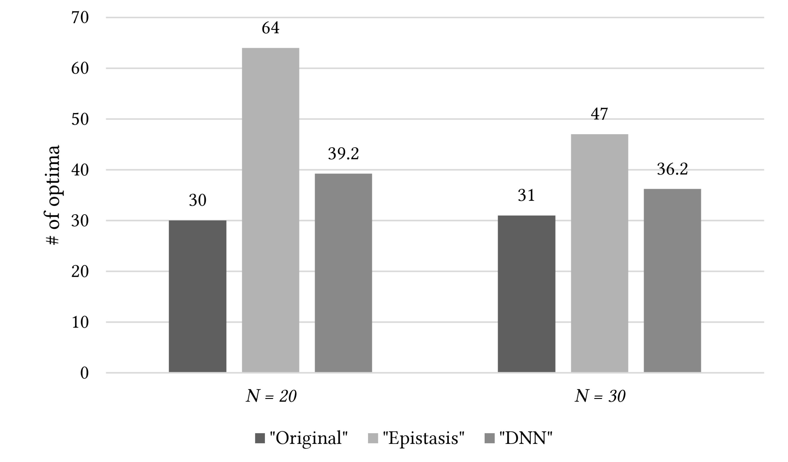
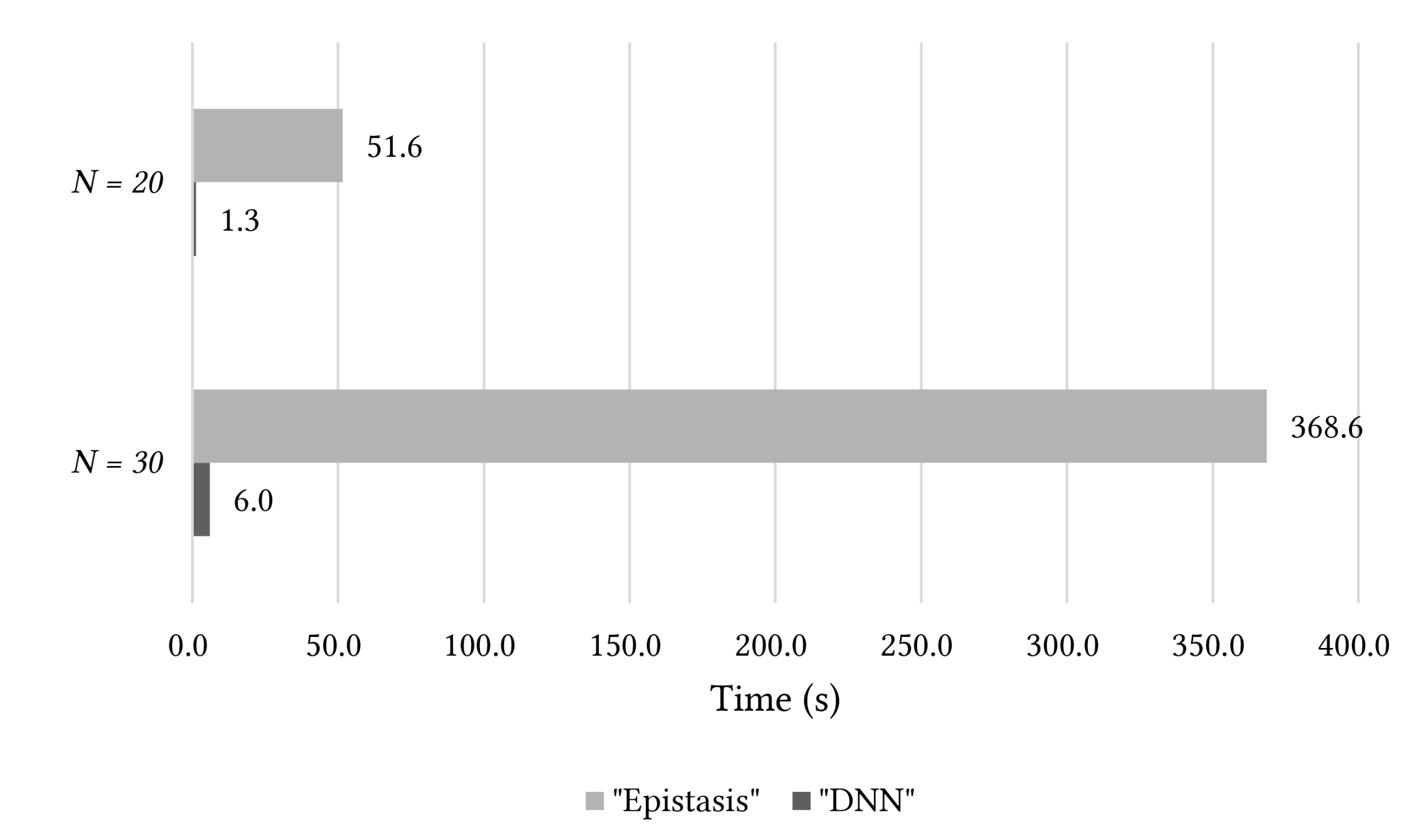
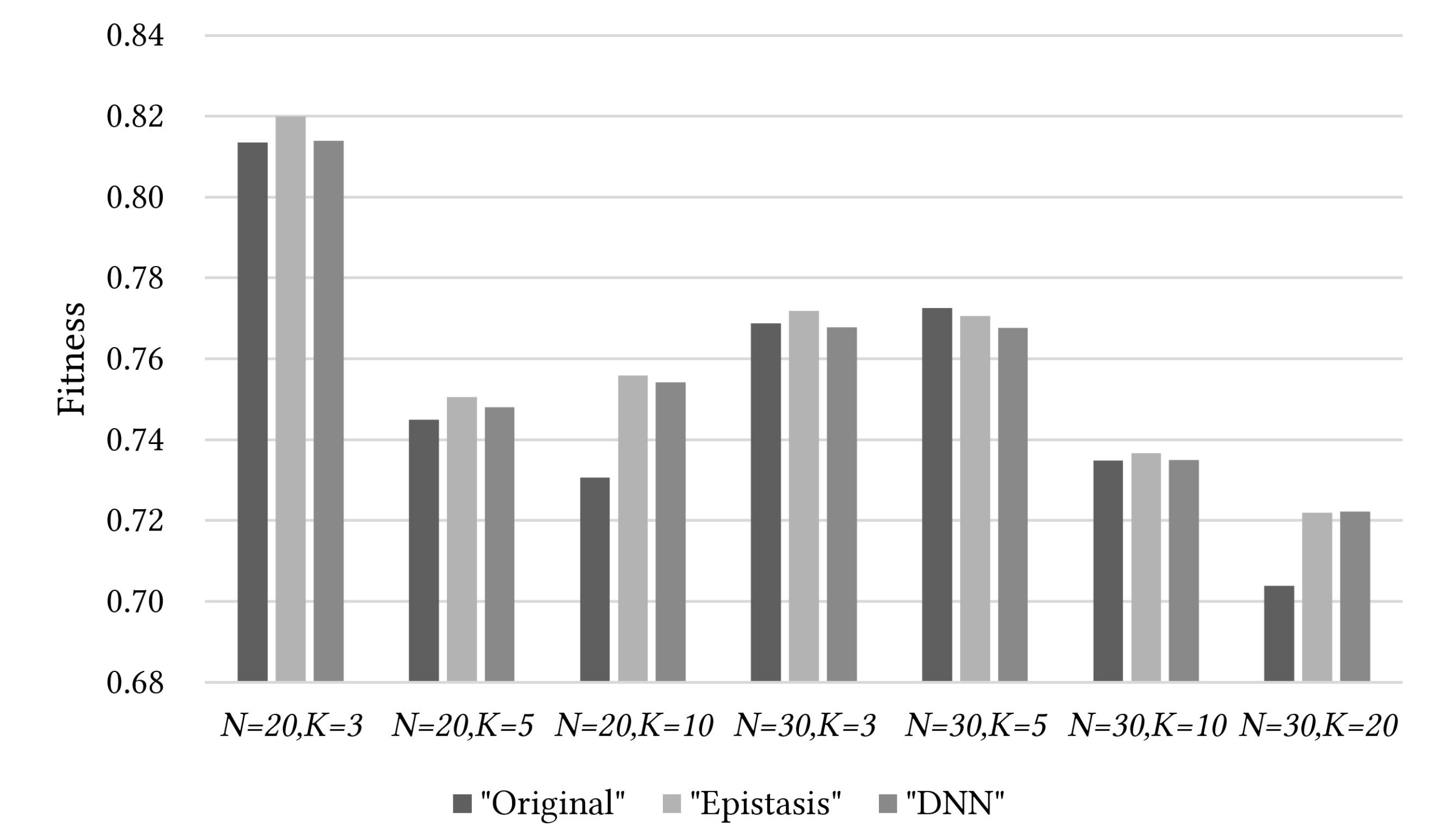
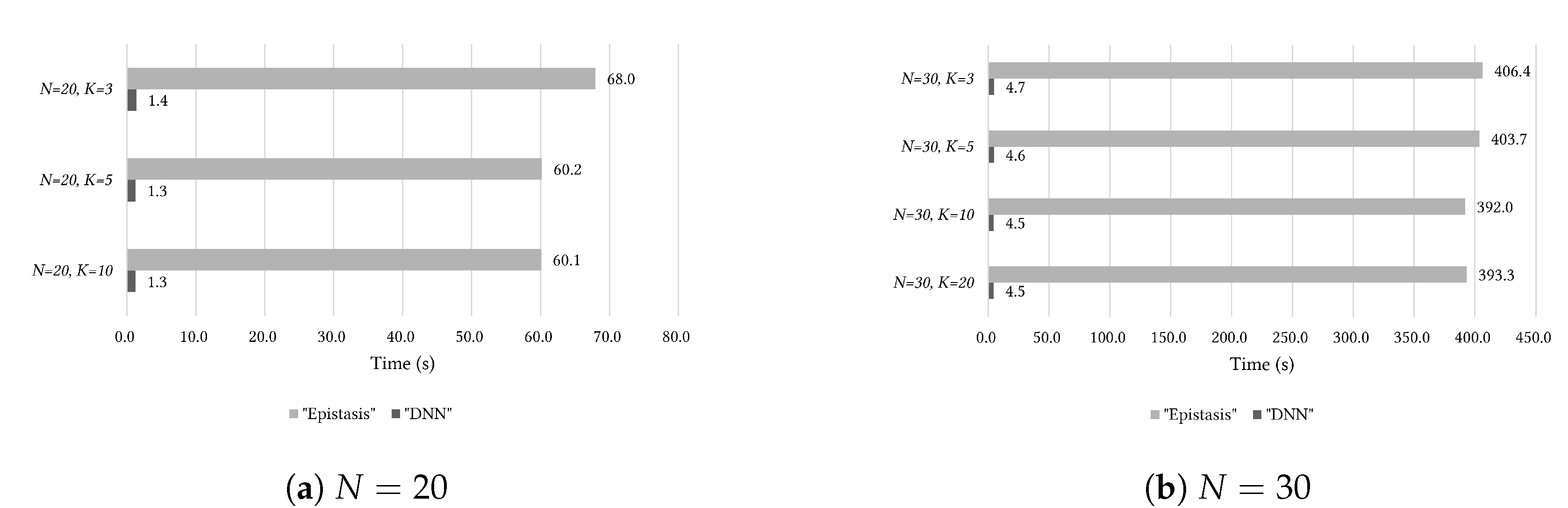
Our experiments were conducted on the computing environments presented in

Table 3. Test environments.

CPU	Intel® CoreTM i7-6850K CPU @ 3.60 GHz
GPU	NVIDIA GeForce GTX 1080 Ti × 4
RAM	64 GB
Operating system	Ubuntu 18.04 LTS
Programing language (version)	Python (3.7)

. Further, GPU computation was used for tensor calculation to reduce the time of the DNN model training. The amount of data was reduced after removing the duplicated data from Table 2. If the training process was conducted repeatedly on a small amount of data, it may result in an overfit. To prevent an overfit, additional data were generated in a manner similar to the one used by Lee and Kim [10]. The amount of data generated for each problem became 100 times the amount of data before the duplication removal; the generated data were then used for the DNN model training.

5.2. Results

We conducted experiments on the Variant-OneMax and $NK$-landscape problems. As shown in Figure 3, the experiments were split into two parts. The first part involved searching for another basis for each problem through a GA, whereas the second part consisted of finding the optimal solution for each problem by changing the basis found through another GA. In this study, we used the DNN model trained by the basis and the epistasis that were used in the experiments by Lee and Kim [10].

On the Variant-OneMax problem, experiments were conducted for $N=20$ and $N=30$. This experiments was conducted under the same conditions as in [41], and the same result was obtained. In both cases, the basis was searched for using a GA. Then, after changing as the basis obtained by the GA, the optimal solution was obtained by independently searching for solutions one hundred times on each of the problem instances. For finding the best solution on the problem, our GA used one-point crossover and bit-flip mutation with probability 0.05. The remaining part including selection and replacement were the same as GA for finding a good basis in Section 4.2. This process was repeated 10 times to obtain the average values.

Table 4. Experimental results on the Variant-OneMax Problem [41].

Trial	Variant-OneMax
	$\mathit{N}=\mathbf{20}$	$\mathit{N}=\mathbf{30}$
1	35	25
2	42	48
3	17	25
4	24	31
5	51	24
6	49	70
7	36	48
8	30	41
9	55	3
10	53	47
Average	39.2	36.2

shows how well the optimal solution could be found when the estimation method using the DNN was applied to the Variant-OneMax problem.

In Figure 4 and Figure 5, “Original” corresponds to the case where the optimal solution is found without applying the basis change. “Epistasis” corresponds to the case of finding the optimal solution using the epistasis-based basis evaluation method proposed by Lee and Kim [10]. “DNN” is the result of applying the method proposed in this study. Considering the results in Figure 4, “Epistasis” provided the best results among all the cases. “DNN” provided better results than “Original”, but performed slightly poorer than “Epistasis.” However, in Table 4, “DNN” showed almost similar results to “Epistasis.” Considering the computation time results in Figure 5, there was a 40 to 60 times difference between “DNN” and “Epistasis.”

On the $NK$-landscape problem, experiments were conducted for seven different cases: ($N=20$, $K=3$), ($N=20$, $K=5$), ($N=20$, $K=10$), ($N=30$, $K=3$), ($N=30$, $K=5$), ($N=30$, $K=10$), and ($N=30$, $K=20$). Similar to the Variant-OneMax problem, the basis was searched for using a GA, following that the change was made on the obtained basis. This was followed by ten repetitions of the independent GA search that was conducted 100 times. The results of the experiments are summarized in

Table 5. Experimental results for the $NK$-landscape problem.

N, K		$\mathit{N}=20$ $\mathit{K}=3$	$\mathit{N}=20$ $\mathit{K}=5$	$\mathit{N}=20$ $\mathit{K}=10$	$\mathit{N}=30$ $\mathit{K}=3$	$\mathit{N}=30$ $\mathit{K}=5$	$\mathit{N}=30$ $\mathit{K}=10$	$\mathit{N}=30$ $\mathit{K}=20$
1	Average	0.8169	0.7445	0.7487	0.7714	0.7655	0.7313	0.7209
	Best	0.8250	0.7613	0.7814	0.7763	0.7952	0.7791	0.7549
2	Average	0.8154	0.7433	0.7572	0.7663	0.7658	0.7388	0.7210
	Best	0.8250	0.7613	0.7855	0.7763	0.7873	0.7745	0.7627
3	Average	0.8141	0.7467	0.7550	0.7625	0.7683	0.7358	0.7240
	Best	0.8250	0.7613	0.7855	0.7763	0.7952	0.8048	0.7615
4	Average	0.8130	0.7533	0.7595	0.7718	0.7643	0.7337	0.7217
	Best	0.8250	0.7613	0.7855	0.7763	0.7897	0.7802	0.7526
5	Average	0.8165	0.7560	0.7563	0.7706	0.7720	0.7338	0.7244
	Best	0.8250	0.7613	0.7855	0.7763	0.7952	0.7804	0.7726
6	Average	0.8137	0.7504	0.7573	0.7700	0.7701	0.7322	0.7215
	Best	0.8250	0.7613	0.7855	0.7763	0.7952	0.8034	0.7627
7	Average	0.8158	0.7463	0.7529	0.7630	0.7701	0.7373	0.7244
	Best	0.8250	0.7613	0.7814	0.7763	0.7952	0.7717	0.7715
8	Average	0.8094	0.7461	0.7540	0.7671	0.7719	0.7323	0.7215
	Best	0.8250	0.7613	0.7855	0.7763	0.7952	0.7855	0.7590
9	Average	0.8091	0.7429	0.7540	0.7678	0.7582	0.7400	0.7216
	Best	0.8250	0.7613	0.7855	0.7763	0.7876	0.7844	0.7525
10	Average	0.8150	0.7501	0.7475	0.7679	0.7706	0.7341	0.7210
	Best	0.8250	0.7613	0.7855	0.7763	0.7952	0.7749	0.7541
Total	Average	0.8139	0.7480	0.7542	0.7678	0.7677	0.7349	0.7222
	Best	0.8250	0.7613	0.7855	0.7763	0.7952	0.8048	0.7726

.

In Figure 6, Figure 7 and Figure 8, “Original,” “Epistasis,” and “DNN” illustrate the same trends as obtained from the Variant-OneMax problem. Figure 6 compares the entire population averages. The best quality of population was obtained when “Epistasis” was used. “DNN” had better results than “Original”, but showed slightly poorer results than “Epistasis.” However, the comparison results for the optimal solutions were more important because the best solution of the population was the optimal solution. In Figure 7, “DNN” generally found better optimal solutions than “Original,” and also found almost identical or slightly poorer solutions when compared with “Epistasis.” In Figure 8, when we compared the computing time taken, “Epistasis” required 46 to 87 times longer times compared with that required by “DNN.”

In this study, it was confirmed only how well the best solution of the problems was found, and we did not perform a statistical analysis. Derrac et al. [45] explained how to use statistical tests to compare evolutionary algorithms. In future work, it is valuable to check the significance of our improvement through a statistical analysis.

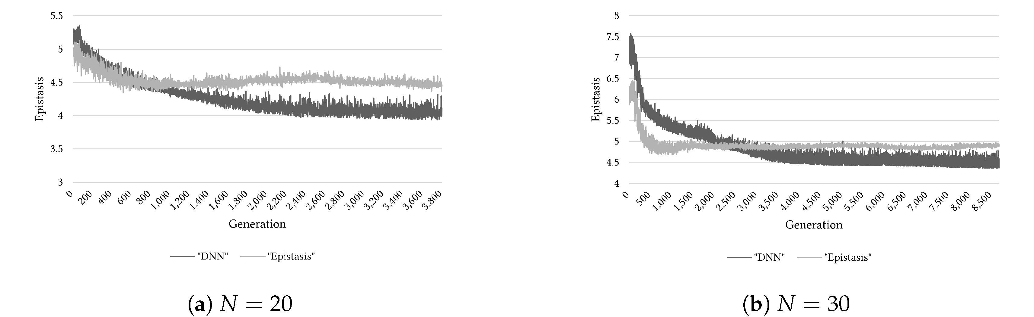
5.3. Epistasis Estimation Based on Basis

This section examines the effectiveness of the epistasis estimation method based on the DNN. Through Figure 9, Figure 10 and Figure 11, we can know the comparison results of estimating the epistasis with the DNN and calculating the epistasis of sampled solutions in the basis search using a GA. Considering Figure 9, the estimation results using the DNN model appeared to be similar to the calculated epistasis for the Variant-OneMax problem. However, from Figure 10 and Figure 11, when we considered the $NK$-landscape problem, the difference between the DNN model estimation and the calculated epistasis is observed to increase with the growth in problem complexity. Owing to this tendency, the reason for the lower quality of the population by “DNN” than that by “Epistasis” for the cases of ($N=30$, $K=10$) and ($N=30$, $K=20$) can be guessed as follows. As the Variant-OneMax problem is a relatively simple problem, the epistasis estimation based on the basis was not presented with any significant difficulties; however, on the $NK$-landscape problem, as the problem complexity increased, the estimation by the DNN became more difficult.

6. Conclusions

Lee and Kim [10] introduced an epistasis-based basis evaluation method; in this study, however, we propose a surrogate model-based epistasis estimation method, which uses deep neural networks (DNNs) for epistasis estimation.The proposed method was applied to two types of problems, as discussed in Section 2.6, then experiments were conducted. The results were compared with those obtained using the epistasis-based basis evaluation method. Regarding the optimal solution search, estimating the epistasis of the basis using the DNN model was nearly always better than that with no basis change. In addition, the method using the DNN showed nearly similar or slightly poorer results than the epistasis-based basis evaluation. In particular, on the $NK$-landscape problem, the method using the DNN provided optimal solutions that were quite similar to those obtained using the epistasis-based basis evaluation. However, using the DNN, the time required for the epistasis estimation was 87 times less as compared with the one conventionally used. Although our method spent time to construct a surrogate model using DNN, the time was just for pre-processing, and it was a low overhead that was much less than the time taken by the previous method [10] that repeatedly calculated epistasis. Therefore, by applying our method, a successful estimation of the epistasis was achieved, along with effective reduction in the computation time. (See Table 2, and Figure 5 and Figure 8).

The contributions of our study can be described as follows. Kim and Yoon [6] presented the effect of basis change. Lee and Kim [9] obtained a good basis by using a meta-GA, and also obtained better results on the $NK$-landscape problem using this basis. However, the meta-GA is time intensive and is therefore very impractical. To address this issue, they proposed an epistasis-based basis evaluation method [10] that showed better efficiency than the meta-GA method; however, their method was still computationally intensive. To this end, we proposed a surrogate model method of estimating the epistasis by using a DNN model. The proposed method showed similar qualities as the epistasis-based basis evaluation method while significantly reducing the computation time. Thus, our epistasis estimation using the DNN was more efficient than the previous methods; furthermore, our method was found to be more practical.

However, the DNN model was presented with challenges when we estimate the epistasis as the problem complexity increased, due to the following reasons: the use of the estimated epistasis values instead of the actual calculated values for DNN training resulted in a lower estimation accuracy, or that each problem required different optimal hyperparameters for the DNN. Thus, in the future, we intend to improve the results of the present study by improving the method of searching for the better optimal solution or by developing separate DNN models for each problem.

References

1. Tripathy, R.K.; Bilionis, I. Deep UQ: Learning deep neural network surrogate models for high dimensional uncertainty quantification. J. Comput. Phys. 2018, 375, 565–588. [Google Scholar] [CrossRef] [Green Version]
2. Pfrommer, J.; Zimmerling, C.; Liu, J.; Kärger, L.; Henning, F.; Beyerer, J. Optimisation of manufacturing process parameters using deep neural networks as surrogate models. Procedia CiRP 2018, 72, 426–431. [Google Scholar] [CrossRef]
3. Mbarek, R.; Tmar, M.; Hattab, H. Vector space basis change in information retrieval. Computación y Sistemas 2014, 18, 569–579. [Google Scholar] [CrossRef]
4. Mbarek, R.; Tmar, M.; Hattab, H. A new relevance feedback algorithm based on vector space basis change. In International Conference on Intelligent Text Processing and Computational Linguistics; Springer: Berlin/Heidelberg, Germany, 2014; pp. 355–366. [Google Scholar]
5. Seo, K.; Hyun, S.; Kim, Y.H. An edge-set representation based on a spanning tree for searching cut space. IEEE Trans. Evol. Comput. 2014, 19, 465–473. [Google Scholar] [CrossRef]
6. Kim, Y.H.; Yoon, Y. Effect of changing the basis in genetic algorithms using binary encoding. KSII Trans. Internet Inf. Syst. 2008, 2. [Google Scholar] [CrossRef]
7. Reeves, C.R.; Wright, C.C. Epistasis in genetic algorithms: An experimental design perspective. In Proceedings of the International Conference on Genetic Algorithms, Pittsburgh, PA, USA, 15–19 July 1995; pp. 217–224. [Google Scholar]
8. Naudts, B.; Kallel, L. A comparison of predictive measures of problem difficulty in evolutionary algorithms. IEEE Trans. Evol. Comput. 2000, 4, 1–15. [Google Scholar] [CrossRef]
9. Lee, J.; Kim, Y.H. Importance of finding a good basis in binary representation. In Proceedings of the Genetic and Evolutionary Computation Conference Companion, Kyoto, Japan, 15–19 July 2018; pp. 49–50. [Google Scholar]
10. Lee, J.; Kim, Y.H. Epistasis-based basis estimation method for simplifying the problem space of an evolutionary search in binary representation. Complexity 2019. [Google Scholar] [CrossRef]
11. Meyer, C.D. Matrix Analysis and Applied Linear Algebra; Siam: Philadelphia, PA, USA, 2000; Volume 71. [Google Scholar]
12. Hirsch, M.W.; Devaney, R.L.; Smale, S. Differential Equations, Dynamical Systems, and Linear Algebra; Academic Press: Cambridge, MA, USA, 1974; Volume 60. [Google Scholar]
13. Davidor, Y. Epistasis variance: Suitability of a representation to genetic algorithms. Complex Syst. 1990, 4, 369–383. [Google Scholar]
14. LeCun, Y.; Bengio, Y.; Hinton, G. Deep learning. Nature 2015, 521, 436–444. [Google Scholar] [CrossRef]
15. LeCun, Y.; Bottou, L.; Bengio, Y.; Haffner, P. Gradient-based learning applied to document recognition. Proc. IEEE 1998, 86, 2278–2324. [Google Scholar] [CrossRef] [Green Version]
16. Rumelhart, D.E.; Hinton, G.E.; Williams, R.J. Learning representations by back-propagating errors. Nature 1986, 323, 533–536. [Google Scholar] [CrossRef]
17. Smolensky, P. Information Processing in Dynamical Systems: Foundations of Harmony Theory; Technical Report; Colorado Univ at Boulder Dept of Computer Science: Boulder, CO, USA, 1986. [Google Scholar]
18. Ong, Y.S.; Nair, P.B.; Keane, A.J. Evolutionary optimization of computationally expensive problems via surrogate modeling. AIAA J. 2003, 41, 687–696. [Google Scholar] [CrossRef] [Green Version]
19. Sreekanth, J.; Datta, B. Multi-objective management of saltwater intrusion in coastal aquifers using genetic programming and modular neural network based surrogate models. J. Hydrol. 2010, 393, 245–256. [Google Scholar] [CrossRef]
20. Eason, J.; Cremaschi, S. Adaptive sequential sampling for surrogate model generation with artificial neural networks. Comput. Chem. Eng. 2014, 68, 220–232. [Google Scholar] [CrossRef]
21. Lim, D.; Jin, Y.; Ong, Y.S.; Sendhoff, B. Generalizing surrogate-assisted evolutionary computation. IEEE Trans. Evol. Comput. 2009, 14, 329–355. [Google Scholar] [CrossRef] [Green Version]
22. Amouzgar, K.; Bandaru, S.; Ng, A.H. Radial basis functions with a priori bias as surrogate models: A comparative study. Eng. Appl. Artif. Intell. 2018, 71, 28–44. [Google Scholar] [CrossRef]
23. Kattan, A.; Galvan, E. Evolving radial basis function networks via GP for estimating fitness values using surrogate models. In Proceedings of the IEEE Congress on Evolutionary Computation, Brisbane, Australia, 10–15 June 2012. [Google Scholar]
24. Lange, K.; Hunter, D.R.; Yang, I. Optimization transfer using surrogate objective functions. J. Comput. Graph. Stat. 2000, 9, 1–20. [Google Scholar]
25. Manzoni, L.; Papetti, D.M.; Cazzaniga, P.; Spolaor, S.; Mauri, G.; Besozzi, D.; Nobile, M.S. Surfing on fitness landscapes: A boost on optimization by Fourier surrogate modeling. Entropy 2020, 22, 285. [Google Scholar] [CrossRef] [Green Version]
26. Yu, D.P.; Kim, Y.H. Predictability on performance of surrogate-assisted evolutionary algorithm according to problem dimension. In Proceedings of the Genetic and Evolutionary Computation Conference Companion, Prague, Czech Republic, 13–17 July 2019; pp. 91–92. [Google Scholar]
27. Verel, S.; Derbel, B.; Liefooghe, A.; Aguirre, H.; Tanaka, K. A surrogate model based on Walsh decomposition for pseudo-Boolean functions. In International Conference on Parallel Problem Solving from Nature; Springer: Berlin/Heidelberg, Germany, 2018; pp. 181–193. [Google Scholar]
28. Leprêtre, F.; Verel, S.; Fonlupt, C.; Marion, V. Walsh functions as surrogate model for pseudo-Boolean optimization problems. In Proceedings of the Genetic and Evolutionary Computation Conference, Prague, Czech Republic, 13–17 July 2019; pp. 303–311. [Google Scholar]
29. Swingler, K. Learning and searching pseudo-Boolean surrogate functions from small samples. Evol. Comput. 2020, 28, 317–338. [Google Scholar] [CrossRef]
30. Zhu, Y.; Zabaras, N. Bayesian deep convolutional encoder–decoder networks for surrogate modeling and uncertainty quantification. J. Comput. Phys. 2018, 366, 415–447. [Google Scholar] [CrossRef] [Green Version]
31. Zhu, Y.; Zabaras, N.; Koutsourelakis, P.S.; Perdikaris, P. Physics-constrained deep learning for high-dimensional surrogate modeling and uncertainty quantification without labeled data. J. Comput. Phys. 2019, 394, 56–81. [Google Scholar] [CrossRef] [Green Version]
32. Karavolos, D.; Liapis, A.; Yannakakis, G.N. Using a surrogate model of gameplay for automated level design. In Proceedings of the 2018 IEEE Conference on Computational Intelligence and Games (CIG), Maastricht, The Netherlands, 14–17 August 2018; pp. 1–8. [Google Scholar]
33. Melo, A.; Cóstola, D.; Lamberts, R.; Hensen, J. Development of surrogate models using artificial neural network for building shell energy labelling. Energy Policy 2014, 69, 457–466. [Google Scholar] [CrossRef] [Green Version]
34. Kourakos, G.; Mantoglou, A. Pumping optimization of coastal aquifers based on evolutionary algorithms and surrogate modular neural network models. Adv. Water Resour. 2009, 32, 507–521. [Google Scholar] [CrossRef]
35. Kim, H.J.; Kim, Y.H. A Surrogate Model Using Deep Neural Networks for Optimal Oil Skimmer Assignment. In Proceedings of the Genetic and Evolutionary Computation Conference Companion, Cancun, Mexico, 8–12 July 2020; pp. 39–40. [Google Scholar]
36. Kauffman, S.A.; Weinberger, E.D. The NK model of rugged fitness landscapes and its application to maturation of the immune response. J. Theor. Biol. 1989, 141, 211–245. [Google Scholar] [CrossRef]
37. Weinberger, E.D. NP Completeness of Kauffman’S NK Model, a Tuneably Rugged Fitness Landscape; Santa Fe Institute Technical Reports; Santa Fe Institute: Santa Fe, NM, USA, 1996. [Google Scholar]
38. Yoon, Y.; Kim, Y.H. A mathematical design of genetic operators on GLn(2). Math. Probl. Eng. 2014, 2014. [Google Scholar] [CrossRef] [Green Version]
39. Wagner, R.A.; Fischer, M.J. The string-to-string correction problem. J. ACM (JACM) 1974, 21, 168–173. [Google Scholar] [CrossRef]
40. Kim, Y.H.; Lee, J.; Kim, Y.H. Predictive model for epistasis-based basis evaluation on pseudo-Boolean function using deep neural networks. In Proceedings of the Genetic and Evolutionary Computation Conference Companion, Prague, Czech Republic, 13–17 July 2019; pp. 61–62. [Google Scholar]
41. Kim, Y.H.; Kim, Y.H. Finding a better basis on binary representation through DNN-based epistasis estimation. In Proceedings of the Genetic and Evolutionary Computation Conference Companion, Cancun, Mexico, 8–12 July 2020; pp. 229–230. [Google Scholar]
42. Dahl, G.E.; Sainath, T.N.; Hinton, G.E. Improving deep neural networks for LVCSR using rectified linear units and dropout. In Proceedings of the IEEE International Conference on Acoustics, Speech and Signal Processing, Vancouver, BC, Canada, 26–31 May 2013; pp. 8609–8613. [Google Scholar]
43. Glorot, X.; Bengio, Y. Understanding the difficulty of training deep feedforward neural networks. In Proceedings of the Thirteenth International Conference on Artificial Intelligence and Statistics, Sardinia, Italy, 13–15 May 2010; pp. 249–256. [Google Scholar]
44. He, K.; Zhang, X.; Ren, S.; Sun, J. Delving deep into rectifiers: Surpassing human-level performance on imagenet classification. In Proceedings of the IEEE International Conference on Computer Vision, Santiago, Chile, 7–13 December 2015; pp. 1026–1034. [Google Scholar]
45. Derrac, J.; García, S.; Molina, D.; Herrera, F. A practical tutorial on the use of nonparametric statistical tests as a methodology for comparing evolutionary and swarm intelligence algorithms. Swarm Evol. Comput. 2011, 1, 3–18. [Google Scholar] [CrossRef]
Figure 1. Structure of the CNN model used in this study, when N = 20 .
Mathematics 08 01287 g001
Figure 2. Flowchart of our genetic algorithm (GA) [10] combined with the proposed surrogate model.
Mathematics 08 01287 g002
Figure 3. Flowchart of a GA (right-side solid box) with a change of basis which is found by another GA (left-side dotted box).
Mathematics 08 01287 g003
Figure 4. Performance comparison of the experiment in this study (“DNN”) and those in previous studies (“Original” and “Epistasis”) on the Variant-OneMax problem [41].
Mathematics 08 01287 g004
Figure 5. Comparison of processing time for the experiment in this study (“DNN”) and that in previous study (“Epistasis”) on the Variant-OneMax problem [41].
Mathematics 08 01287 g005
Figure 6. Performance comparison of the experiment in this study (“DNN”) and those in previous studies (“Original” and “Epistasis”) on the average of population for the N K -landscape problem.
Mathematics 08 01287 g006
Figure 7. Comparison of best solution results for the experiments in this study (“DNN”) and previous studies (“Original” and “Epistasis”) on the N K -landscape problem.
Mathematics 08 01287 g007
Figure 8. Comparison of processing time for the experiments in this study (“DNN”) and previous study (“Epistasis”) on the NK-landscape problem.
Mathematics 08 01287 g008
Figure 9. Comparison of target epistasis values (“Epistasis”) and ones estimated by DNN (“DNN”) on the Variant-OneMax problem.
Mathematics 08 01287 g009
Figure 10. Comparison of target epistasis values (“Epistasis”) and ones estimated by DNN (“DNN”) on the N K -landscape problem ( N = 20 ).
Mathematics 08 01287 g010aMathematics 08 01287 g010b
Figure 11. Comparison of target epistasis values (“Epistasis”) and ones estimated by DNN (“DNN”) on the NK-landscape problem ( K = 30 ).
Mathematics 08 01287 g011