Magnetohydrodynamic Flow and Heat Transfer Induced by a Shrinking Sheet


Abstract
1. Introduction
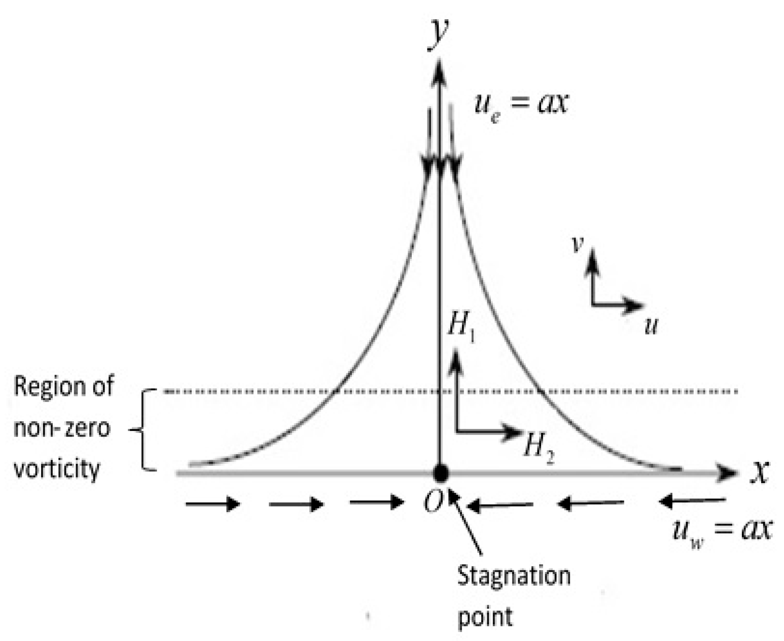
2. Basic Equations
3. Flow Stability
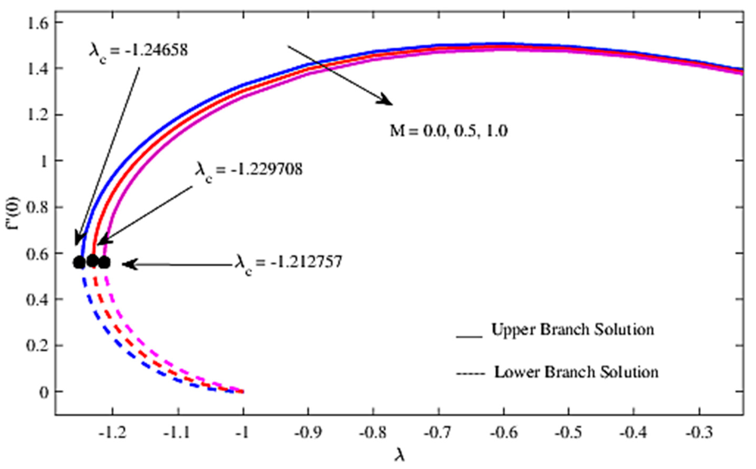
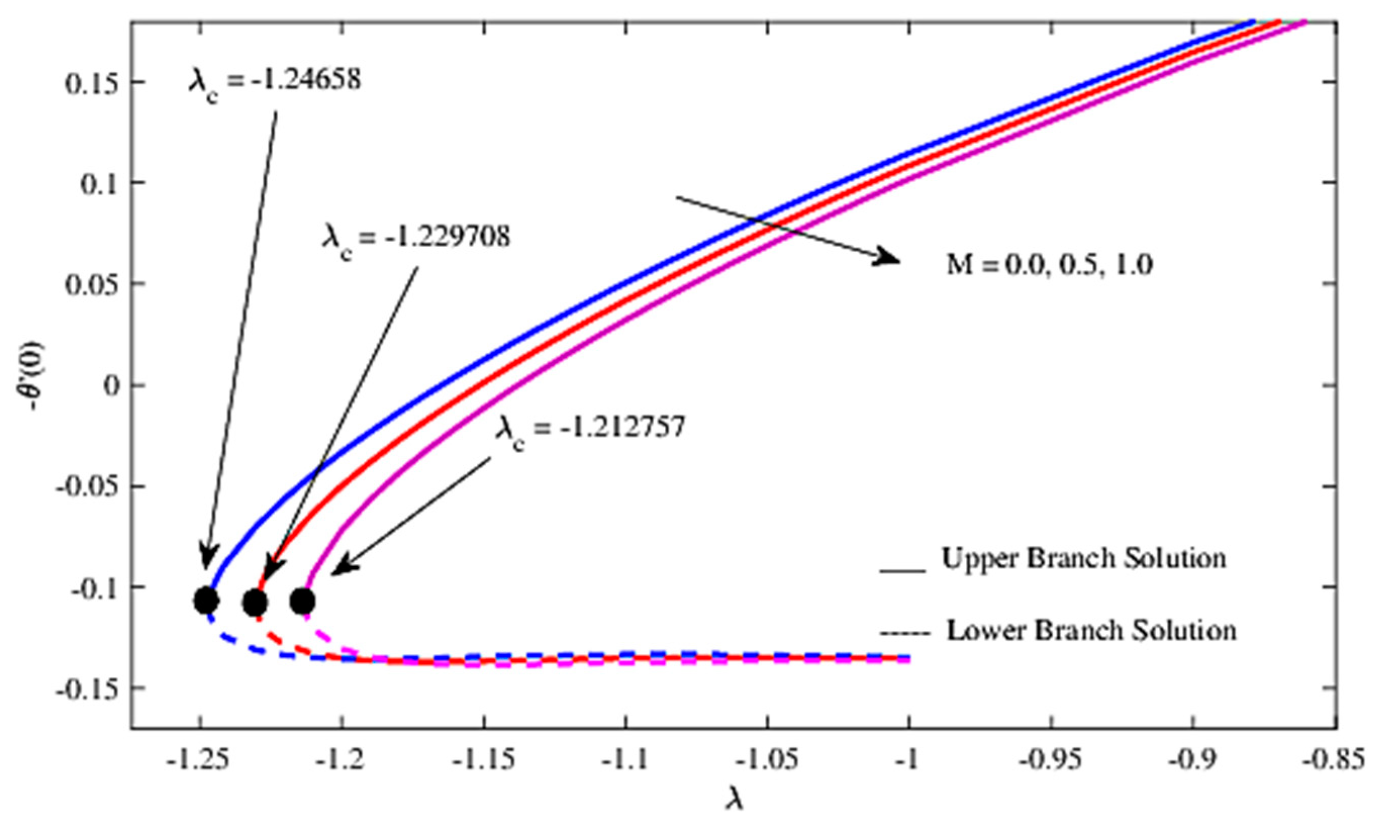
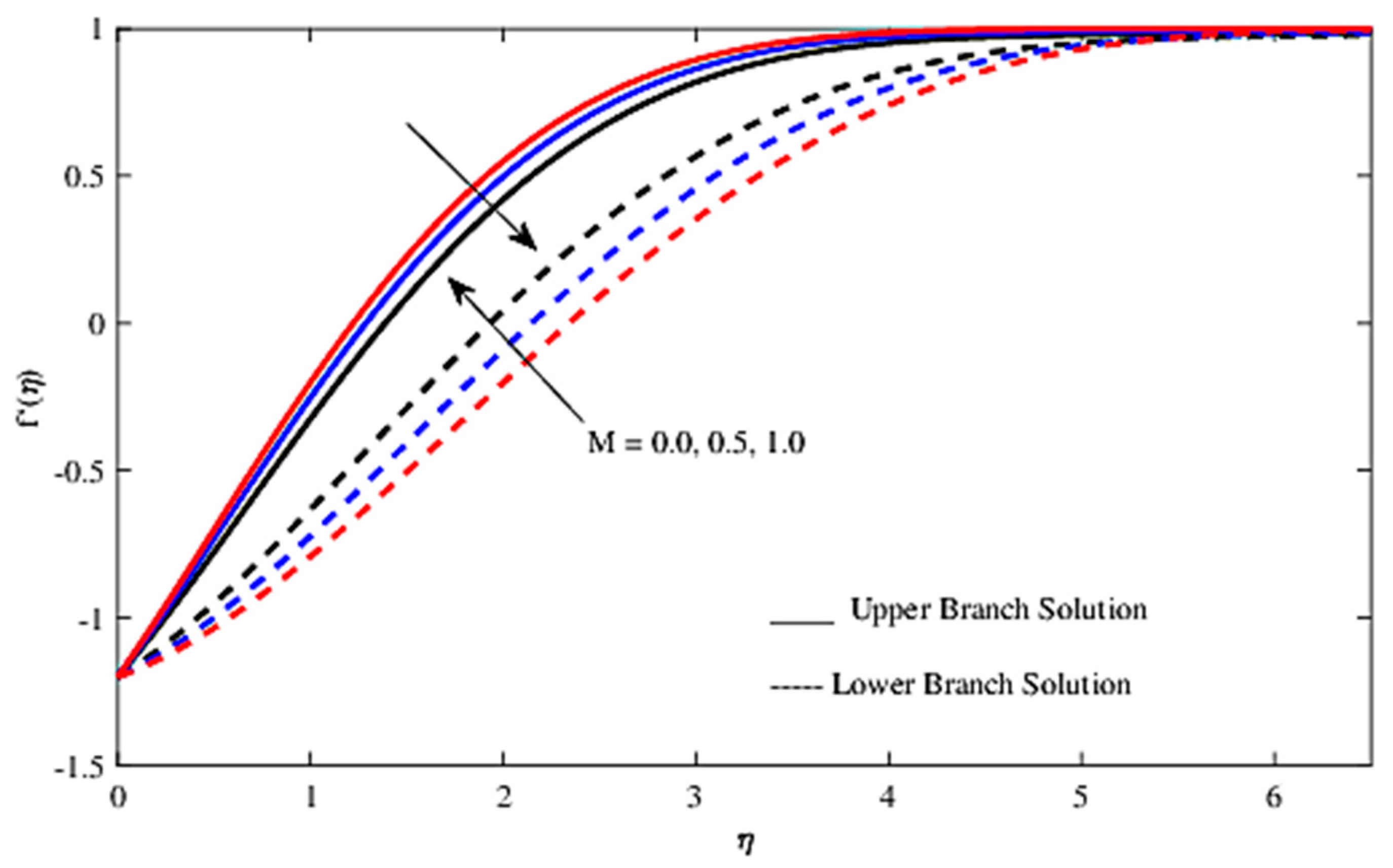
4. Result and Discussion
5. Conclusions
Author Contributions
Funding
Acknowledgments
Conflicts of Interest
Nomenclatures
| Cf | Skin friction coefficient |
| cp | Specific heat at constant pressure (JKg−1 K−1) |
| ρcp | Heat capacitance of the fluid (JK−1 m−3) |
| f(η) | Dimensionless stream function |
| H0 | Initial velocity magnetic field |
| H1, H2 | Velocity magnetic field component in x and y direction |
| He | Velocity magnetic field of the ambient fluid |
| Nux | Local Nusselt number |
| Pr | Prandtl number |
| Q0 | Thermal conductivity |
| Rex | Local Reynolds number |
| T | Fluid temperature (K) |
| Tw | Surface temperature (K) |
| T∞ | Ambient temperature (K) |
| T | Time (s) |
| U, V | Velocity component time dependent in the x and y directions (ms−1) |
| u, v | Velocity components in the x and y directions (ms−1) |
| uw | Velocity of the surface (ms−1) |
| ue | Ambient velocity (ms−1) |
| Greek symbols | |
| α | Thermal diffusivity |
| γ | Eigenvalue |
| ζ0 | Magnetic diffusivity |
| η | Similarity variable |
| λ | Shrinking parameter |
| θ | Dimensionless temperature |
| μ | Dynamic viscosity of the fluid (kgm−1s−1) |
| ν | Kinematic viscosity of the fluid (m2 s−1) |
| ρ | Density of the fluid (kgm−3) |
| τw | Skin friction or wall shear stress (kgm−1s−2) |
| τ | Dimensionless time |
| Subscripts | |
| f | Fluid |
| Superscript | |
| ‘ | Differentiation with respect to η |
References
- Rashad, A.M. Impact of thermal radiation on MHD slip flow of a ferrofluid over a non-isothermal wedge. J. Magn. Magn. Mater. 2017, 422, 25–31. [Google Scholar] [CrossRef]
- Hassan, M.; Marin, M.; Alsharif, A.; Ellahi, R. Convection heat transfer flow of nanofluid in a porous medium over wavy surface. Phys. Lett. A 2018, 382, 2749–2753. [Google Scholar] [CrossRef]
- Jha, B.K.; Aina, B. Role of induced magnetic field on MHD natural convection flow in vertical microchannel formed by two electrically non-conducting infinite vertical parallel plates. Alex. Eng. J. 2016, 55, 2087–2097. [Google Scholar] [CrossRef]
- Fang, T. Magnetohydrodynamic viscous flow over a nonlinearly moving surface: Closed-form solutions. Eur. Phys. J. Plus 2014, 129, 92. [Google Scholar] [CrossRef]
- Goldsworthy, F.A. Magnetohydrodynamic flow of a perfectly conducting, viscous fluid. J. Fluid Mech. 1961, 11, 519–528. [Google Scholar] [CrossRef]
- Zhang, J.; Fang, T.; Zhong, Y.F. Analytical solution of magnetohydrodynamic sink flow. Appl. Math. Mech. Engl. 2011, 32, 1221–1230. [Google Scholar] [CrossRef]
- Alamri, S.Z.; Khan, A.A.; Azeez, M.; Ellahi, R. Effects of mass transfer on MHD second grade fluid towards stretching cylinder: A novel perspective of Cattaneo-Christov heat flux model. Phys. Lett. A 2019, 383, 276–281. [Google Scholar] [CrossRef]
- Yousif, M.A.; Ismael, H.K.; Abbas, T.; Ellahi, R. Numerical study of momentum and heat transfer of MHD Carreaunanofluid over an exponentially stretched plate with internal heat source/sink and radiation. Heat Transf. Res. 2019, 50, 649–658. [Google Scholar] [CrossRef]
- Fang, T.; Zhang, J.; Yao, S. Slip MHD viscous flow over a stretching sheet—An exact solution. Commun. Nonlinear Sci. Numer. Simul. 2009, 14, 3731–3737. [Google Scholar] [CrossRef]
- Fang, T.; Zhang, J. Closed-form exact solutions of MHD viscous flow over a shrinking sheet. Commun. Nonlinear Sci. Numer. Simul. 2009, 14, 2853–2857. [Google Scholar] [CrossRef]
- Nandy, S.K.; Sidui, S.; Mahapatra, T.R. Unsteady MHD boundary-layer flow and heat transfer of nanofluid over a permeable shrinking sheet in the presence of thermal radiation. Alex. Eng. J. 2014, 53, 929–937. [Google Scholar] [CrossRef]
- Akbar, N.S.; Nadeem, S.; Ul-Haq, R.; Yex, S. MHD stagnation point flow of Carreau fluid toward a permeable shrinking sheet: Dual solutions. Ain Shams Eng. J. 2014, 5, 1233–1239. [Google Scholar] [CrossRef]
- Ghosh, S.; Mukhopadhyay, S.; Vajravelu, K. Dual solutions of slip flow past a nonlinearly shrinking permeable sheet. Alex. Eng. J. 2016, 55, 1835–1840. [Google Scholar] [CrossRef]
- Nadeem, S.; Ul-Haq, R.; Lee, C. MHD flow of a Casson fluid over an exponentially shrinking sheet. Sci. Iran. 2012, 19, 1550–1553. [Google Scholar] [CrossRef]
- Rosali, H.; Ishak, A.; Nazar, R.; Pop, I. Rotating flow over an exponentially shrinking sheet with suction. J. Mol. Liq. 2015, 211, 965–969. [Google Scholar] [CrossRef]
- Rosca, N.C.; Rosca, A.V.; Pop, I. Lie group symmetry method for MHD double-diffusive convection from a permeable vertical stretching/shrinking sheet. Comput. Math. Appl. 2016, 71, 1679–1693. [Google Scholar] [CrossRef]
- Turkyilmazoglu, M. MHD fluid flow and heat transfer due to a shrinking rotating disk. Comput. Fluids 2014, 90, 51–56. [Google Scholar] [CrossRef]
- Soid, S.K.; Ishak, A.; Pop, I. Unsteady MHD flow and heat transfer over a shrinking sheet with ohmic heating. Chin. J. Phys. 2017, 55, 1626–1636. [Google Scholar] [CrossRef]
- Fang, T.; Wang, F. Viscous slip MHD flow over a moving sheet with an arbitrary surface velocity. Chin. Phys. Lett. 2018, 35, 104701. [Google Scholar] [CrossRef]
- Hiemenz, K. Die grenzschicht an einem in den gleichformingen flussigkeitsstrom eingetauchten geraden kreiszylinder. Dinglers Polytech. J. 1911, 326, 321–324. [Google Scholar]
- Mustafa, I.; Javed, T.; Ghaffari, A. Heat transfer in MHD stagnation point flow of a ferrofluid over a stretchable rotating disk. J. Mol. Liq. 2016, 219, 526–532. [Google Scholar] [CrossRef]
- Ibrahim, W. The effect of induced magnetic field and convective boundary condition on MHD stagnation point flow and heat transfer of upper-convected Maxwell fluid in the presence of nanoparticle past a stretching sheet. Propuls. Power Res. 2016, 5, 164–175. [Google Scholar] [CrossRef]
- Mabood, F.; Khan, W.A.; Ismail, A.M. MHD stagnation point flow and heat transfer impinging on stretching sheet with chemical reaction and transpiration. Chem. Eng. J. 2015, 273, 430–437. [Google Scholar] [CrossRef]
- Farooq, M.; Khan, M.I.; Waqas, M.; Hayat, T.; Alsaedi, A.; Khan, M.I. MHD stagnation point flow of viscoelastic nanofluid with non-linear radiation effects. J. Mol. Liq. 2016, 221, 1097–1103. [Google Scholar] [CrossRef]
- Rostami, M.N.; Dinarvand, S.; Pop, I. Dual solutions for mixed convective stagnation-point flow of an aqueous silica-alumina hybrid nanofluid. Chin. J. Phys. 2018, 56, 2465–2478. [Google Scholar] [CrossRef]
- Nasir, N.A.A.M.; Ishak, A.; Pop, I. Stagnation-point flow and heat transfer past a permeable quadratically stretching/shrinking sheet. Chin. J. Phys. 2017, 55, 2081–2091. [Google Scholar] [CrossRef]
- Khan, M.I.; Kiyani, M.Z.; Malik, M.Y.; Yasameen, T.; Khan, M.W.A.; Abbas, T. Numerical investigation of magnetohydrodynamic stagnation point flow with variable properties. Alex. Eng. J. 2016, 55, 2367–2373. [Google Scholar] [CrossRef]
- Ali, F.M.; Nazar, R.; Arifin, N.M.; Pop, I. MHD boundary layer flow and heat transfer over a stretching sheet with induced magnetic field. Heat Mass Transf. 2011, 47, 155–162. [Google Scholar] [CrossRef]
- Ali, F.M.; Nazar, R.; Arifin, N.M.; Pop, I. MHD stagnation-point flow and heat transfer towards stretching sheet with induced magnetic field. Appl. Math. Mech. Engl. 2011, 32, 409–418. [Google Scholar] [CrossRef]
- Goldstein, S. On backward boundary layers and flow in converging passage. J. Fluid Mech. 1965, 21, 33–45. [Google Scholar] [CrossRef]
- Cowling, T.G. Magnetohydrodynamics; Interscience Publishers: New York, NY, USA; London, UK, 1957. [Google Scholar]
- Mahapatra, T.R.; Gupta, A.S. Heat transfer in stagnation-point flow towards a stretching sheet. Heat Mass Transf. 2002, 38, 517–521. [Google Scholar] [CrossRef]
- Zeeshan, A.; Shehzad, N.; Abbas, T.; Ellahi, R. Effects of radiative electro-Magnetohydrodynamics diminishing internal energy of pressure-driven flow of titanium dioxide-water nanofluid due to entropy generation. Entropy 2019, 21, 236. [Google Scholar] [CrossRef]
- Weidman, P.D.; Kubitschek, D.G.; Davis, A.M.J. The effect of transpiration on self similar boundary layer flow over moving surfaces. Int. J. Eng. Sci. 2006, 44, 730–737. [Google Scholar] [CrossRef]
- Rosca, N.C.; Pop, I. Mixed convection stagnation point flow past a vertical flat plate with a second order slip: Heat flux case. Int. J. Heat Mass Transf. 2013, 65, 102–109. [Google Scholar] [CrossRef]
- Waini, I.; Ishak, A.; Pop, I. Squeezed hybrid nanofluid flow over a permeable sensor surface. Mathematics 2020, 8, 898. [Google Scholar] [CrossRef]
- Harris, S.D.; Ingham, D.B.; Pop, I. Mixed convection boundary-layer flow near the stagnation point on a vertical surface in a porous medium: Brinkman model with slip. Transp. Porous Media 2009, 77, 267–285. [Google Scholar] [CrossRef]
- Rosca, A.V.; Rosca, N.C.; Pop, I. Numerical simulation of the stagnation point flow past a permeable stretching/shrinking sheet with convective boundary condition and heat generation. Int. J. Numer. Methods Heat 2016, 26, 348–364. [Google Scholar] [CrossRef]
- Ishak, A.; Lok, Y.Y.; Pop, I. Stagnation-point flow over a shrinking sheet in a micropolar fluid. Chem. Eng. Commun. 2010, 197, 1417–1427. [Google Scholar] [CrossRef]
- Takhar, H.S.; Chamkha, A.J.; Nath, G. Unsteady flow and heat transfer on a semi-infinite at plate with an aligned magnetic. Int. J. Eng. Sci. 1999, 37, 1723–1736. [Google Scholar] [CrossRef]
- Sarafraz, M.M.; Pourmehran, O.; Yang, B.; Arjomandi, M.; Ellahi, R. Pool boiling heat transfer characteristics of iron oxide nano-suspension under constant magnetic field. Int. J. Therm. Sci. 2020, 147, 106131. [Google Scholar] [CrossRef]
- Dhanai, R.; Rana, P.; Kumar, L. MHD mixed convection nanofluid flow and heat transfer over an inclined cylinder due to velocity and thermal slip effects: Buongiorno’s model. Powder Technol. 2016, 288, 140–150. [Google Scholar] [CrossRef]


| λ | Present Study | Ishak et al. [39] | Rosca et al. [38] | |||
|---|---|---|---|---|---|---|
| Upper Branch | Lower Branch | Upper Branch | Lower Branch | Upper Branch | Lower Branch | |
| −0.5 | 1.495690 | - | 1.495670 | - | 1.495669 | - |
| −0.75 | 1.489298 | - | 1.489298 | - | 1.489298 | - |
| −1 | 1.328817 | 0.0 | 1.328817 | 0.0 | 1.328816 | 0.0 |
| −1.15 | 1.082231 | 0.116702 | 1.082231 | 0.116702 | 1.082231 | 0.116702 |
| −1.20 | 0.932473 | 0.233650 | 0.932474 | 0.233650 | 0.932473 | 0.233649 |
| M | Re(1/2)xCf | Re(−1/2)xNux | ||
|---|---|---|---|---|
| Upper Branch | Lower Branch | Upper Branch | Lower Branch | |
| 0.1 | 0.919288600 | 0.245461561 | 0.036388462 | 0.135535051 |
| 0.5 | 0.860316623 | 0.299225512 | 0.049914145 | 0.135168459 |
| 1.0 | 0.761569269 | 0.392040873 | 0.071787829 | 0.130550670 |
| Q | 0 | 0.2 | 0.5 | |
|---|---|---|---|---|
| Re(−1/2)xNux | Upper branch solution | −0.093149185 | 0.194299118 | 1.160454023 |
| Lower branch solution | −0.002856956 | 0.304206653 | 1.362866119 | |
© 2020 by the authors. Licensee MDPI, Basel, Switzerland. This article is an open access article distributed under the terms and conditions of the Creative Commons Attribution (CC BY) license (http://creativecommons.org/licenses/by/4.0/).
Share and Cite
Mohd Nasir, N.A.A.; Ishak, A.; Pop, I. Magnetohydrodynamic Flow and Heat Transfer Induced by a Shrinking Sheet. Mathematics 2020, 8, 1175. https://doi.org/10.3390/math8071175
Mohd Nasir NAA, Ishak A, Pop I. Magnetohydrodynamic Flow and Heat Transfer Induced by a Shrinking Sheet. Mathematics. 2020; 8(7):1175. https://doi.org/10.3390/math8071175
Chicago/Turabian StyleMohd Nasir, Nor Ain Azeany, Anuar Ishak, and Ioan Pop. 2020. "Magnetohydrodynamic Flow and Heat Transfer Induced by a Shrinking Sheet" Mathematics 8, no. 7: 1175. https://doi.org/10.3390/math8071175
APA StyleMohd Nasir, N. A. A., Ishak, A., & Pop, I. (2020). Magnetohydrodynamic Flow and Heat Transfer Induced by a Shrinking Sheet. Mathematics, 8(7), 1175. https://doi.org/10.3390/math8071175