The Effects of Icing on Aircraft Longitudinal Aerodynamic Characteristics

Abstract

To study the effects of ice accretion on the longitudinal aerodynamic characteristics of an aircraft, a two-part method for predicting longitudinal aerodynamic derivatives of iced aircraft is proposed. For the aircraft with a flight test, a parameter identification system based on maximum likelihood criterion and a longitudinal nonlinear flight dynamics model is established. For the aircraft without a flight test, an engineering prediction method of aerodynamic derivatives based on an individual component CFD calculation and narrow strip theory is established. According to the flight test data of DHC-6 Twin Otter aircraft from NASA, the longitudinal aerodynamic parameters of both clean and artificially iced aircraft are obtained. Additionally, the longitudinal aerodynamic derivatives of the iced aircraft are calculated. Then, the correctness of the prediction method is verified by comparing the calculated results with the identification results. The comparison of these results shows that the prediction method is correct and accurate, and it can be used to calculate the effects of icing on the aircraft longitudinal aerodynamic parameters.

1. Introduction

Aircraft icing is the phenomena of ice accretion on the aircraft. Aircraft icing will change the air flow around the lift surface, thus reducing the performance and control ability of the aircraft. Severe icing will cause air separation on the airfoil ahead of time, resulting in a stall [1], which poses a threat to the safety of flight characteristics. In order to prevent the serious consequences of icing, an anti-icing system is usually installed on the important lifting components of modern aircraft. However, flights with ice accretion on the aircraft are still unavoidable, and the accidents are usually caused by the failure or improper operation of ice protection systems. According to the data given by National Transportation Safety Board (NTSB) [2], from 1981 to 1988, about 542 aircraft accidents are caused by aircraft icing. According to the statistics of the International Civil Aviation Organization (ICAO), the death rate of passengers in aircraft icing accidents reached 39% in the early 1990s [3]. Aircraft icing is still a big problem for flight safety and the studies on this area are attracting more attention.

In order to define the effects of ice accretion on aircraft, the methods of parameter identification were used to extract the aerodynamic parameters from flight test data. Ranaudo et al. [4] compared the stability and control derivatives between clean and naturally iced aircraft, using a modified maximum likelihood estimation method with flight test data of Twin Otter. Ratvasky and Ranaudo [5] studied the effects of ice accretion on Twin Otter stability and control derivatives with flight test data of clean and artificially iced aircraft, and a modified stepwise regression algorithm was used to obtain pitching and yawing derivatives. Whalen [6], based on the flight test data of Twin Otter, studied the changes of stability and control derivatives of naturally iced aircraft from clean aircraft with a MATLAB toolbox called System Identification Programs for Aircraft (SIDPAC) [7], and an analysis was given about the differences of aerodynamic parameters with different icing locations on aircraft. Melody et al. [8] compared the results of different parameter identification techniques: a batch least-squares algorithm, an extended Kalman filter, and an $H^{\infty }$ algorithm, and found that only the $H^{\infty }$ method provides a timely and accurate icing indication.

Flight test data and identification results of icing could be used as a basis component of the forecast of aircraft icing. Based on the flight test data of the Twin Otter aircraft [4,5,9], Bragg [10] proposed a simple model to relate ice accretion effects with icing and flight parameters, which could be used on the Twin Otter aircraft to sense the effect of ice accretion on the aircraft performance and control during quasi-steady-state flight. Lampton [11] developed a methodology and simulation tool for evaluation of aircraft dynamical response, stability and control characteristics due to icing. The component build-up method was used to implement icing effects. Based on the flight test data from the Tailplane Icing Program (TIP) [12] conducted by National Aeronautics and Space Administration (NASA) and Federal Aviation Administration (FAA), Hiltner et al. [13] developed an analytical tool called TAILSIM to model the effects of tailplane icing on the flight dynamics of the Twin Otter aircraft and a comparison has been made between the responses of the TAILSIM program and the flight test data. Di Donato et al. [14] studied the viability of ice accretion detection using measurements of a single output from airplane longitudinal dynamics, and a parameter estimation method is used to detect the changes due to ice accretion. Ratvasky et al. [15], in 2008, reviewed the methods available to model and simulate icing effects on performance, stability and control, including the wind tunnel testing of sub-scale complete aircraft models, which showed that modeling and simulating methods could help to forecast the effects of aircraft icing. Deiler [16] presented a new Δ model approach to model the icing-related degradation of aircraft aerodynamics, which described changes of the longitudinal and lateral aircraft aerodynamics accurately.

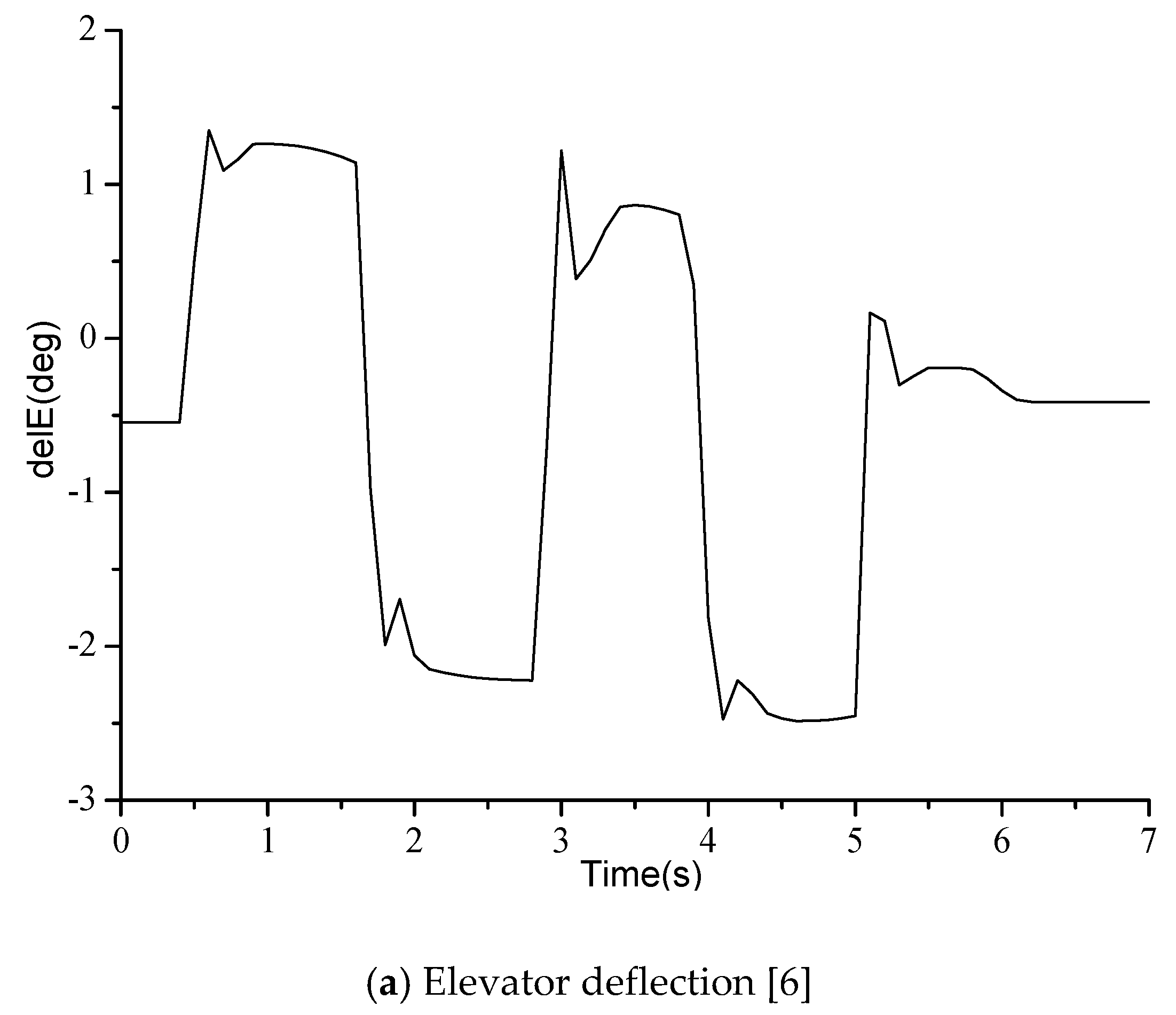
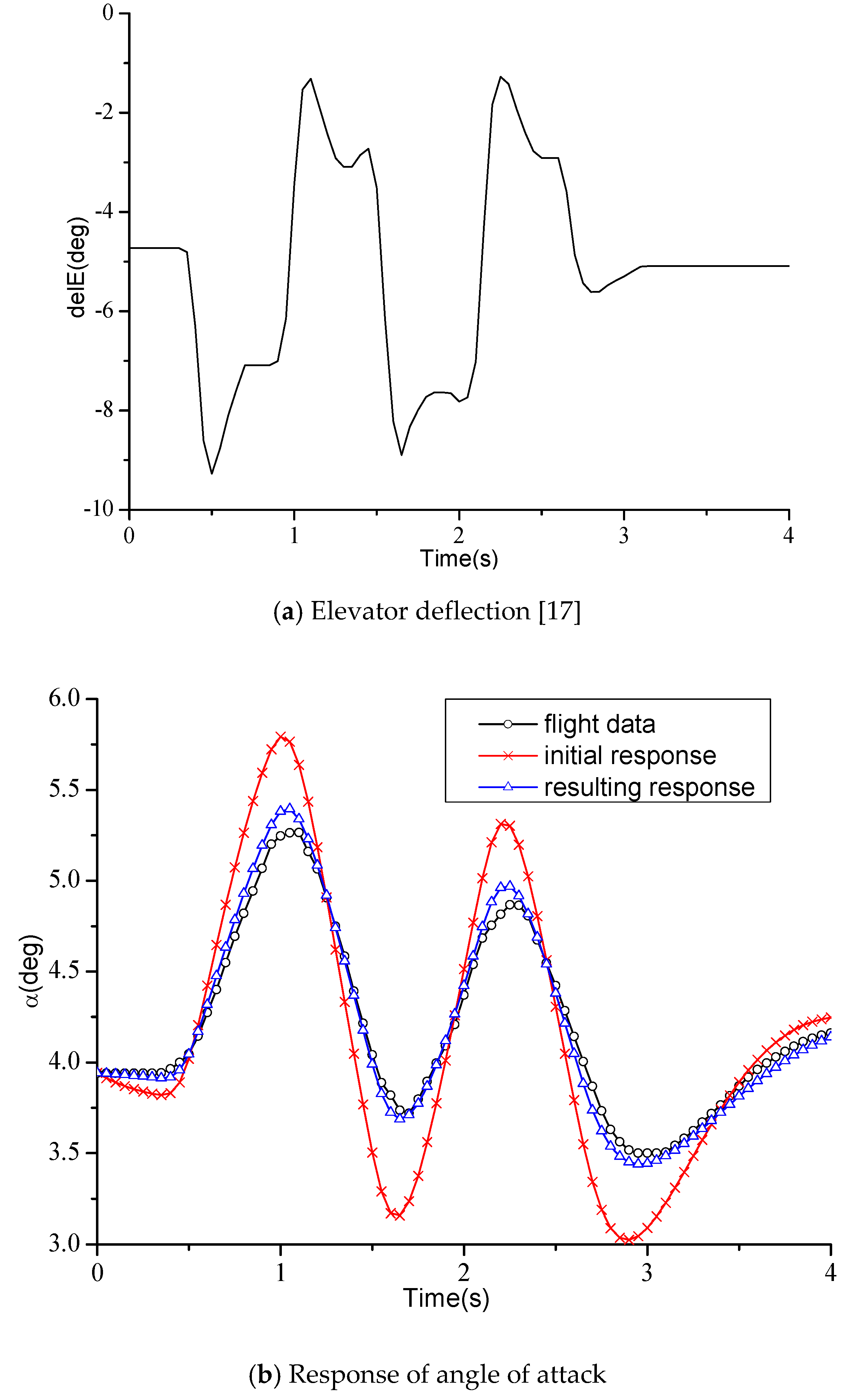
In this paper, a two-part method for predicting longitudinal aerodynamic derivatives of iced aircraft is proposed. Firstly, a nonlinear modeling of longitudinal flight dynamics is carried out. Then, for the aircraft with flight test, a parameter identification system based on maximum likelihood criterion is established. Furthermore, according to the NASA flight test data [17,18], the longitudinal aerodynamic parameters of both clean and artificially iced aircraft are obtained by the maximum likelihood identification method. Finally, for the aircraft without flight test, an engineering prediction method of aerodynamic derivatives based on individual component CFD calculation and narrow strip theory is established. The longitudinal aerodynamic derivatives are calculated by the prediction method, and the correctness of the prediction method is verified by comparing the calculated results with the identified results.

The contribution of this paper is the establishment of a reasonable and accurate method for calculating the effects of icing on aircraft longitudinal aerodynamic parameters. Based on the ice shapes of wing and horizontal tail, this approach can easily calculate the difference between clean and iced aircrafts. The utility of this approach is the ability to evaluate the effects of different ice shapes accreted on the wing or horizontal tail of the aircraft, especially for those where icing data do not exist. Usually, the complete CFD method needs to calculate the ice shape according to the meteorological conditions, then grid the aircraft model and, finally, carry out the flow numerical simulation. The method in this paper only needs to calculate the aerodynamic derivatives of individual aircraft component. Compared with the complete CFD method, this method reduces a lot of calculation and can provide fast estimation results for engineering.

2. Theories and Calculation Methods

2.1. Aircraft Dynamic Model

Parameter identification is to solve the related parameters of a system when the input and output of the system are known. To describe the system, a mathematical model is built first. According to the characteristics of an iced aircraft, a nonlinear longitudinal flight dynamics model is constructed.

$$\{\begin{array}{l}\dot{\overrightarrow{x}}(t)=f(\overrightarrow{x}(t),\overrightarrow{u}(t),t)\\ \overrightarrow{x}(t)={[u,w,q,\theta ,x_e,h]}^T\\ \overrightarrow{u}(t)={[{\delta }_e,{\delta }_T]}^T\end{array}$$

(1)

where the state vector $\overrightarrow{x}(t)$ includes forward velocity $u$, angular velocity $w, q,$ the Euler angle $\theta$ and spatial position coordinates $x_e, h$. The control vector $\overrightarrow{u}(t)$ includes the elevator deflection ${\delta }_e$ and engine thrust ${\delta }_T$.

Figure 1 shows the coordinate systems of longitudinal motion of airplane, where ox_b and oz_b are the body axes, ox_E and oz_E are the earth axes.

$$\left[\begin{array}{l}{x}_e\\ h\end{array}\right]=L_{Eb}\left[\begin{array}{l}u\\ w\end{array}\right]$$

(2)

where $L_{Eb}$ is the transfer matrix from the body coordinate system to earth’s coordinate system.

Generally, aircraft is regarded as a rigid body when analyzing the whole motion of aircraft. The nonlinear ordinary differential motion equations are as follows:

$$\{\begin{array}{l}\dot{u}=\frac{F_X}{m}-qw\\ \dot{w}=\frac{F_Z}{m}+qu\\ \dot{q}=\frac{M}{I_Y}\end{array}$$

(3)

The aerodynamic model is as following:

$$\{\begin{array}{l}{C}_X=C_{X0}+C_{X\alpha 2}{\alpha }^2\\ C_Z=C_{Z0}+C_{Z\alpha }\alpha +C_{Zq}q\frac{\overline{c}}{2V}+C_{Z\delta e}{\delta }_e\\ C_m=C_{m0}+C_{m\alpha }\alpha +C_{mq}q\frac{\overline{c}}{2V}+C_{m\delta e}{\delta }_e\end{array}$$

(4)

where, $C_{X0}$, $C_{X\alpha 2}$, $C_{Z0}$, $C_{Z\alpha }$, $C_{Zq}$, $C_{Z\delta e}$, $C_{m0}$, $C_{m\alpha }$, $C_{mq}$, $C_{m\delta e}$ are unknown aerodynamic derivatives, that is, the target of parameter identification.

2.2. Parameter Identification Method

After the aircraft dynamic model is established, the unknown parameters of the model, namely aerodynamic derivative, need to be identified. In this paper, the maximum likelihood criterion is used to identify the parameters.

The dynamic system model can be written as follows:

$$\{\begin{array}{l}\dot{\overrightarrow{x}} (t)=f[ \overrightarrow{x}(t), \overrightarrow{u}(t), \overrightarrow{\lambda }, t ], \overrightarrow{x}(t_0)={\overrightarrow{x}}_0\\ \overrightarrow{y} (t)=h [ \overrightarrow{x}(t), \overrightarrow{u}(t), \overrightarrow{\lambda }, t ]\\ \overrightarrow{v} (i)=\overrightarrow{z} (i)-\overrightarrow{y} (i)\end{array}$$

(5)

where, $\overrightarrow{x}$ is the state vector, $\overrightarrow{u}$ is the input vector, $\overrightarrow{\lambda }$ is the parameter vector to be identified, $\overrightarrow{z}$ is the test data vector, $\overrightarrow{y}$ is the observation vector, $\overrightarrow{v}$ is the difference between $\overrightarrow{z}$ and $\overrightarrow{y}$, and i represents the number of times.

The theory of parameter identification proves that the maximum likelihood estimation of parameters is asymptotically unbiased, consistent and effective. When the experimental data of the system are enough, the mathematical expectation of the parameters obtained by the maximum likelihood identification is the true value and converges to the true value with probability 1. Its variance gradually reaches the Cramer-Rao lower bound, which is the unbiased estimation with the minimum variance. Therefore, the maximum likelihood estimation of the parameters is to seek the parameters to minimize the following likelihood indicator functions.Indicator function of the maximum likelihood identification is:

$$J={\displaystyle \sum _{i=1}^N[\overrightarrow{v}{(i)}^T{B}^{-1}\overrightarrow{v}(i)+\ln \left|B\right|]}$$

(6)

where B is the innovation variance matrix. The optimal estimation $\widehat{B}$ of B can be obtained by finding the extremum of J to B.

$$\widehat{B}=\frac{1}{N} {\displaystyle \sum _{i=1}^N\overrightarrow{v}(i) \overrightarrow{v}{(i)}^T}$$

(7)

Then, the asymptotically unbiased, uniform and efficient estimation of $\overrightarrow{\lambda }$ can be obtained by minimizing J to $\overrightarrow{\lambda }$. The iterative convergence process of $\overrightarrow{\lambda }$ is based on the modified Newton-Raphon algorithm [19].

The procedure of the identification program is shown in Figure 2.

2.3. The Prediction Method

The maximum likelihood identification method is introduced to identify the mathematical model under aircraft icing in Section 2.2. However, this method strongly relies on the flight test, whenever the ice shapes have a large change the identification results maybe heavily discounted. Therefore, based on the values of clean aircraft’s longitudinal aerodynamic derivatives and the ice shapes of wing and horizontal tail, a prediction method is established to calculate the longitudinal aerodynamic derivatives of $C_{Z\alpha }$, $C_{Zq}$, $C_{Z\delta e}$, $C_{m\alpha }$, $C_{mq}$ and $C_{m\delta e}$. The correctness of the prediction method will be verified by comparing the calculated results with the identified results.

The aerodynamic force in z direction on clean aircraft could be expressed as following:

$$Z=Z_W+Z_F+Z_H+Z_{W(\mathrm{int}er)}+Z_{F(\mathrm{int}er)}+Z_{H(\mathrm{int}er)}$$

(8)

where $Z_{(\mathrm{int}er)}$ is the interference aerodynamic force caused by other part of aircraft components.

The aerodynamic force in Z direction on aircraft with iced wing and horizontal tail could be expressed as following:

$$Z_{(ice)}=Z_{W(ice)}+Z_F+Z_{H(ice)}+Z_{W(\mathrm{int}er,ice)}+Z_{F(\mathrm{int}er,ice)}+Z_{H(\mathrm{int}er,ice)}$$

(9)

Assume that the changes of aerodynamic force on body and the mutual influence of aircraft components caused by icing could be ignored, that is:

$$Z_{W(\mathrm{int}er)}=Z_{W(\mathrm{int}er,ice)},Z_{F(\mathrm{int}er)}=Z_{F(\mathrm{int}er,ice)},Z_{H(\mathrm{int}er)}=Z_{H(\mathrm{int}er,ice)}$$

(10)

Then, Equation (11) can be obtained from Equations (8)–(10).

$$Z_{ice}-Z=(Z_{W(ice)}-Z_W)+(Z_{H(ice)}-Z_H)$$

(11)

namely,

$$q_{\infty (ice)}\cdot C_{Z(ice)}-q_{\infty }\cdot C_Z=(q_{\infty (ice)}\cdot C_{ZW(ice)}-q_{\infty }\cdot C_{ZW})+(k_{q(ice)}\cdot q_{\infty (ice)}\cdot C_{ZH(ice)}-k_q\cdot q_{\infty }\cdot C_{ZH})$$

(12)

where $k_{q(ice)}$ and $k_q$ represent the ratios between the dynamic pressure on the horizontal tail and the wing, and the estimation method from [20] is used to calculate them.

Obtain the partial derivatives of Equation (12) with respect to $\alpha$, $\delta e$ and $q$, separately, and ignore the effects of them on $k_{q(ice)}$ and $k_q$. Then Equation (13) could be achieved.

$$\{\begin{array}{l}{q}_{\infty (ice)}\cdot {(C_{Z\alpha })}_{ice}-q_{\infty }\cdot C_{Z\alpha }=\left[q_{\infty (ice)}\cdot {(C_{Z\alpha })}_{W(ice)}-q_{\infty }\cdot {(C_{Z\alpha })}_W\right]+\left[k_{q(ice)}\cdot q_{\infty (ice)}\cdot {(C_{Z\alpha })}_{H(ice)}-k_q\cdot q_{\infty }\cdot {(C_{Z\alpha })}_H\right]\\ q_{\infty (ice)}\cdot {(C_{Z\delta e})}_{ice}-q_{\infty }\cdot C_{Z\delta e}=k_{q(ice)}\cdot q_{\infty (ice)}\cdot {(C_{Z\delta e})}_{H(ice)}-k_q\cdot q_{\infty }\cdot {(C_{Z\delta e})}_H\\ q_{\infty (ice)}\cdot {(C_{Zq})}_{ice}-q_{\infty }\cdot C_{Zq}=\left[q_{\infty (ice)}\cdot {(C_{Zq})}_{W(ice)}-q_{\infty }\cdot {(C_{Zq})}_W\right]+\left[k_{q(ice)}\cdot q_{\infty (ice)}\cdot {(C_{Zq})}_{H(ice)}-k_q\cdot q_{\infty }\cdot {(C_{Zq})}_H\right]\end{array}$$

(13)

Assume that the changes of $C_{Z\alpha }$, $C_{Z\delta e}$ and $C_{Zq}$ caused by the change of $q_{\infty }$ could be ignored in a certain range. Suppose that

$$q_{\infty }=q_{\infty (ice)}$$

(14)

In addition, because $k_q$ is the ratios of dynamic pressure $q_{\infty }$ and it is assumed that the dynamic pressure $q_{\infty }$ is constant before and after icing. The effects of icing on $k_q$ could be ignored, namely,

$$k_q=k_{q(ice)}$$

(15)

Substituting Equations (14) and (15) into (13), Equation (16) could be obtained.

$$\{\begin{array}{l}{(C_{Z\alpha })}_{ice}-C_{Z\alpha }=\left[{(C_{Z\alpha })}_{W(ice)}-{(C_{Z\alpha })}_W\right]+k_{q(ice)}\left[{(C_{Z\alpha })}_{H(ice)}-{(C_{Z\alpha })}_H\right]\\ {(C_{Z\delta e})}_{ice}-C_{Z\delta e}=k_{q(ice)}\left[{(C_{Z\delta e})}_{H(ice)}-{(C_{Z\delta e})}_H\right]\\ {(C_{Zq})}_{ice}-C_{Zq}=\left[{(C_{Zq})}_{W(ice)}-{(C_{Zq})}_W\right]+k_{q(ice)}\left[{(C_{Zq})}_{H(ice)}-{(C_{Zq})}_H\right]\end{array}$$

(16)

In a similar manner to the upper derivation, Equation (17) could be obtained.

$$\{\begin{array}{l}{(C_{m\alpha })}_{ice}-C_{m\alpha }=\left[{(C_{m\alpha })}_{W(ice)}-{(C_{m\alpha })}_W\right]+k_{q(ice)}\left[{(C_{m\alpha })}_{H(ice)}-{(C_{m\alpha })}_H\right]\\ {(C_{m\delta e})}_{ice}-C_{m\delta e}=k_{q(ice)}\left[{(C_{m\delta e})}_{H(ice)}-{(C_{m\delta e})}_H\right]\\ {(C_{mq})}_{ice}-C_{mq}=\left[{(C_{mq})}_{W(ice)}-{(C_{mq})}_W\right]+k_{q(ice)}\left[{(C_{mq})}_{H(ice)}-{(C_{mq})}_H\right]\end{array}$$

(17)

Ignore the change of aerodynamic force location on wing and horizontal tail caused by icing. Equation (18) could be obtained from Equation (17).

$$\{\begin{array}{l}{(C_{m\alpha })}_{ice}-C_{m\alpha }=\frac{L_{WG}}{\overline{c}}\left[{(C_{Z\alpha })}_{W(ice)}-{(C_{Z\alpha })}_W\right]+\frac{L_{HG}}{\overline{c}}{k}_{q(ice)}\left[{(C_{Z\alpha })}_{H(ice)}-{(C_{Z\alpha })}_H\right]\\ {(C_{m\delta e})}_{ice}-C_{m\delta e}=\frac{L_{HG}}{\overline{c}}{k}_{q(ice)}\left[{(C_{Z\delta e})}_{H(ice)}-{(C_{Z\delta e})}_H\right]\\ {(C_{mq})}_{ice}-C_{mq}=\frac{L_{WG}}{\overline{c}}\left[{(C_{Zq})}_{W(ice)}-{(C_{Zq})}_W\right]+\frac{L_{HG}}{\overline{c}}{k}_{q(ice)}\left[{(C_{Zq})}_{H(ice)}-{(C_{Zq})}_H\right]\end{array}$$

(18)

In Equations (16) and (18), to obtain the difference between iced and clean aircraft aerodynamic derivatives, the terms in the right hand of the equation should be solved first. $C_{Z\alpha }$, $C_{Z\delta e}$ could be easily calculated by changing the angle of attack or the elevator location using CFD software.

As for the dynamic derivative of $C_{Zq}$, a calculation method called the ‘strip’ technique developed by [21] is used. The formulas are shown as Equation (19).

$$\{\begin{array}{l}{(C_{Zq})}_W=\frac{1}{L_{WG}\cdot V}\left[-(\frac{4\sin \alpha }{S}){\displaystyle \sum {\overline{C}}_{Z(\alpha )}{}_{{}_W}}(\Delta Yc)X-(\frac{2\cos \alpha }{S}){\displaystyle \sum {(\frac{\partial {\overline{C}}_Z}{\partial \alpha })}_W}(\Delta Yc)X\right]\\ {(C_{Zq})}_H=-2\frac{L_{HG}}{V}\sin \alpha C_{Z{(\alpha )}_H}-\frac{L_{HG}}{V}\cos \alpha {(\frac{\partial C_Z}{\partial \alpha })}_H\end{array}$$

(19)

3. Identification Method Accuracy Verification

In order to verify the accuracy of the identification method, the following steps are taken.

(1)

Choose a set of aerodynamic parameters ${\overrightarrow{\lambda }}_f$ as the reference value under a flight condition within a reasonable range.

(2)

Take ${\overrightarrow{\lambda }}_f$ as the parameters of an aircraft dynamic model to obtain the response of this reference dynamic model under certain elevator inputs. Then, regard the response data as the flight test reference response for identification using in the next step.

(3)

Add a proactive change $\Delta \overrightarrow{\lambda }$ to ${\overrightarrow{\lambda }}_f$, and ${\overrightarrow{\lambda }}_f$ turned into ${\overrightarrow{\lambda }}_0$, which is regarded as the initial value. Start this identification process from the initial value ${\overrightarrow{\lambda }}_0$ using the response data obtained in step 2. The input value ${\overrightarrow{\lambda }}_r$ is calculated iteratively until the input value response is basically consistent with the reference response. Then, the result ${\overrightarrow{\lambda }}_r$ can be achieved.

(4)

By comparing the difference between the identification result and the reference value, the correctness and accuracy of the identification system are verified.

Aircraft DHC-6 Twin Otter [18], a high-wing, twin-engine, commuter-class aircraft, is chosen as the test plane. The initial flight conditions are shown in

Table 1. Initial flight conditions of method validation.

Parameter	Height	Velocity	Angle of Attack	Pitch Angle	Pitch Rate	Thrust Coefficient
Value	900 m	50 m/s	2.6 deg	2.1 deg	1.05 deg/s	0.1

.

The result of aerodynamic parameters is shown in

Table 2. Identification results for method validation.

Aerodynamic Parameter	Reference Values ${\overrightarrow{\mathit{\lambda }}}_{\mathit{f}}$	Initial Value ${\overrightarrow{\mathit{\lambda }}}_{\mathbf{0}}$	Identification Result ${\overrightarrow{\mathit{\lambda }}}_{\mathit{r}}$	Error (%)
$C_{X0}$	−0.040	−0.045	−0.042	5.000
$C_{X\alpha 2}$	4.500	4.900	4.766	5.910
$C_{Z0}$	−0.380	−0.400	−0.386	1.580
$C_{Z\alpha }$	−5.800	−5.000	−5.758	−0.720
$C_{Zq}$	−20.00	−15.00	−22.50	12.50
$C_{Z\delta e}$	−0.600	−0.850	−0.667	11.17
$C_{m0}$	0.010	0.015	0.009	−6.000
$C_{m\alpha }$	−1.300	−1.000	−1.298	−0.150
$C_{mq}$	−35.00	−27.00	−32.85	−6.200
$C_{m\delta e}$	−1.800	−1.300	−1.700	−5.560

, and the output responses fitting curve is shown in Figure 3, respectively.

As shown in Table 2, the results compared extremely well and most of the errors between identification results and reference values are less than 6%. The errors of $C_{Zq}$ and $C_{Z\delta e}$ are larger than others, 12.50% and 11.17%, respectively. However, the change tendency is reasonable.

It could be observed from Figure 3 that the initial responses of angle of attack and pitch rate have some discrepancies as compared with the reference response curve. However, when the system parameters are alternated with the identification result ${\overrightarrow{\lambda }}_r$, the resulting response curves are almost coincident with the reference curves.

According to the verification results, the error of the identification method is within the acceptable range. This method is relatively effective and accurate, and can be used to identify the aircraft longitudinal aerodynamic parameters.

4. Identification Method Application and Result Analysis

4.1. Identification of Clean Aircraft

Firstly, the identification of clean aircraft in doublet pair flight is carried out. The results are used as the basis for analyzing the effect of aircraft icing. The aerodynamic parameters of aircraft DHC-6 are achieved according to the flight test data provided by [6] (Doublet Pair Flight). The initial flight conditions of clean aircraft are shown in

Table 3. Initial flight conditions of clean aircraft.

Parameter	Height	Velocity	Thrust Coefficient
Value	870 m	51 m/s	0.1

and the output responses fitting curves are shown in Figure 4.

Figure 4 shows the responses of the system model obtained by the identification accord quite well with the flight test data. This proves that the aircraft dynamic model established in this paper can simulate DHC-6 aircraft relatively accurately. Furthermore, it proves that this identification method is useful for identifying aerodynamic parameters.

The initial value and identification results are compared in

Table 4. Identification results of the clean aircraft.

Aerodynamic Parameter	Initial Value	Identification Result	Reference [10]	Error %
$C_{X0}$	−0.040	−0.037	−0.410	−9.76
$C_{X\alpha 2}$	4.500	6.691	—	—
$C_{Z0}$	−0.380	−0.379	−0.380	−0.26
$C_{Z\alpha }$	−5.800	−5.640	−5.660	−0.35
$C_{Zq}$	−20.00	−15.75	−19.97	−21.13
$C_{Z\delta e}$	−0.600	−0.812	−0.608	33.55
$C_{m0}$	0.010	0.005	0.008	−37.50
$C_{m\alpha }$	−1.300	−1.446	−1.310	10.38
$C_{mq}$	−35.00	−29.54	−34.20	−13.64
$C_{m\delta e}$	−1.800	−095	−1.740	20.40

. The results reported in [10] are taken as the references.

As shown in Table 4, although the identification results have some discrepancies relative to the initial values, most of the aerodynamic derivatives accord with the reference results quite well.

The causes of the discrepancies may be as follows:

(1)

In different flight tests, the weight and thrust coefficient of DHC-6 aircraft are different.

(2)

In the process of identification, the aircraft dynamic model established in this paper is different from the reference.

4.2. Identification of Horizontal Tail Iced Aircraft

The horizontal tail is the important part of aircraft for the ability to affect aircraft longitudinal control and stability. To study the effect of icing on horizontal tail aerodynamic performance, data from [18] are used, and the ice shapes of “Inter-cycle” and “Stability and Control (S&C)” on the horizontal tail are chosen, as shown in Figure 5. The identification results of clean aircraft in Section 4.1 are used as the initial value.

Inter-cycle ice shape represents ice accretions remaining on the tail between the pneumatic de-ice boot operation. Conditions: V = 135 knots, alpha = −2.9°, Liquid water content (LWC) = 0.5 g/m³, Median volumetric diameter (MVD) = 20 um, T₀ = −4 °C, time = 15 min, with a boot cycle every 3 min [18].

The S&C ice shape is used extensively in NASA’s previous stability and control tests and it is derived from in-flight photos and ADS-4. The aeroperformance characteristics for this ice shape are the worst and nearly identical to the “lewis-ice (LEWICE)” shape. LEWICE shape conditions: V = 120 knots, alpha = −2.9°, LWC = 0.5 g/m³, MVD = 20 um, T₀ =−4 °C, time = 45 min [18].

Table 5. Initial flight conditions of horizontal tail iced aircraft.

Ice Shape	Height	Velocity	Thrust Coefficient
Inter-cycle	1890 m	70 m/s	0.1
S&C	1850 m	62 m/s	0.1

shows the initial flight conditions of horizontal tail iced aircraft. The fitting curves of the output responses of the aircraft with two different ice shapes are shown in Figure 6, and the result of aerodynamic parameters are shown in

Table 6. Identification results of the horizontal tail iced aircraft.

Aerodynamic Parameter	Clean Aircraft	Inter-Cycle Ice Shape	Change %	S&C Ice Shape	Change %
$C_{X0}$	−0.037	−0.047	27.03	−0.049	33.24
$C_{X\alpha 2}$	6.691	6.749	0.870	6.905	3.20
$C_{Z0}$	−0.379	−0.378	−0.260	−0.375	−1.06
$C_{Z\alpha }$	−5.640	−5.498	−2.520	−5.454	−3.30
$C_{Zq}$	−15.75	−13.52	−14.19	−9.457	−39.96
$C_{Z\delta e}$	−0.812	−0.509	−37.32	−0.431	−46.92
$C_{m0}$	0.005	0.005	6.000	0.0075	50.00
$C_{m\alpha }$	−1.446	−1.282	−11.34	−1.386	−4.150
$C_{mq}$	−29.54	−25.22	−14.62	−23.55	−20.27
$C_{m\delta e}$	−2.095	−1.681	−19.76	−1.649	−21.29

, respectively.

According to the identification results of the two kind of horizontal tail iced aircraft as shown in Table 6, the following analysis could be made.

(1)

Compared with clean aircraft, the absolute value of $C_{X0}$ increases by 27.03% and 33.24%, respectively, under the condition of horizontal tail with two ice shapes. This means that aircraft icing will greatly increase aircraft drag. The absolute values of $C_{Z0}$ and $C_{Z\alpha }$ are slightly reduced, which indicates that horizontal tail icing will lead to a small reduction of lift.

(2)

The absolute value of $C_{mq}$ changes largely under icing conditions with Inter-cycle ice shape and S&C ice shape, by −14.62% and −20.27%, respectively, which means the horizontal tail icing would cause the decrease of pitching damping.

(3)

Relative to the clean aircraft, the absolute values of $C_{Z\delta e}$ and $C_{m\delta e}$ for S&C ice shape condition change significantly by −46.92% and −21.29% respectively, which indicates that horizontal tail icing contributes significantly to the reduction of elevator effectiveness.

(4)

Comparing the identification results under the two different icing conditions, the aerodynamic parameters with S&C ice shape changes larger than those with Inter-cycle ice shape, which means horizontal tail iced aircraft with the ice shape of S&C is more affected.

4.3. Identification of All Configuration Iced Aircraft

Identification of all configuration iced aircraft is studied in this section. With the aerodynamic parameters of clean aircraft in Section 4.1 as the initial values and the flight test operation (Elevator Doublet) in [17] as the input values, the aerodynamic parameters of “all iced” aircraft are identified. These flight tests were conducted with the whole iced configuration of Twin Otter’s aircraft, including the wing, horizontal tail, and vertical tail. The ice shapes of those plans could be found from [17] as shown in Figure 7.

The initial flight conditions of “all iced” aircraft are shown in

Table 7. Initial flight conditions of “all iced” aircraft.

Parameter	Height	Velocity	Thrust Coefficient
Value	1200 m	55 m/s	0.14

. This initial flight conditions are quite close to the conditions of clean aircraft, which will help to get a better identification result. The output responses fitting curves are shown in Figure 8, and the identification results are shown in

Table 8. Identification results of artificially iced aircraft.

Aerodynamic Parameter	Clean Aircraft (Initial Value)	“All Iced” Aircraft			Changes of Horizontal Tail Iced Aircraft
		Identification Result	Change (%)	Reference [9]	S&C	Inter–Cycle
$C_{X0}$	−0.037	−0.062	67.57	−0.062	33.24	27.03
$C_{X\alpha 2}$	6.691	6.591	−1.490	—	3.200	0.870
$C_{Z0}$	−0.379	−0.347	−8.440	−0.380	−1.060	−0.260
$C_{Z\alpha }$	−5.640	−5.294	−6.130	−5.094	−3.300	−2.520
$C_{Zq}$	−15.75	−13.85	−12.06	−19.70	−39.96	−14.19
$C_{Z\delta e}$	−0.812	−0.606	−25.37	−0.550	−46.92	−37.32
$C_{m0}$	0.005	0.003	−40.00	0.008	50.00	6.000
$C_{m\alpha }$	−1.446	−1.008	−30.29	−1.180	−4.150	−11.34
$C_{mq}$	−29.50	−25.35	−14.10	−33.00	−20.27	−14.62
$C_{m\delta e}$	−2.095	−1.621	−22.60	−1.566	−21.29	−19.76

, respectively.

According to the identification results of artificially iced aircraft as shown in Table 8, the following analysis could be made.

(1)

Under an “all iced” condition, the absolute value of $C_{X0}$ increased by 67.57%. The absolute values of $C_{Z0}$ and $C_{Z\alpha }$ decreased by −8.44% and −6.13%, respectively. Compared with the horizontal tail icing condition, these parameters change more. The change range is more than twice. The results show that the main wing icing plays a leading role in the change of aircraft lift and drag characteristics under icing conditions.

(2)

The changes of $C_{Zq}$ and $C_{mq}$ do not reflect great difference compared with horizontal tail iced aircraft, which means when the airplane has a tail, the wing contribute to $C_{Zq}$ and $C_{mq}$ is often negligible in comparison with that of tail [22].

(3)

$C_{m\alpha }$ changes largely under “all iced” condition by −30.29%, while those of horizontal tail iced condition with S&C and Inter-cycle ice shape are −4.15% and −11.34%, respectively. These results indicate that wing icing contributes more to the change of $C_{m\alpha }$.

(4)

The changes of $C_{Z\delta e}$ and $C_{m\delta e}$ under the “all iced” condition are slightly more than those under a horizontal tail iced condition, which indicate that horizontal tail icing mainly contributes to the reduction of elevator effectiveness.

Although the results of this identification method are well fitted with the experimental results and have high accuracy, there are some limitations. This identification method is highly dependent on flight test. When the aircraft configuration is different from that of the identification model, or the ice shape is greatly changed, the accuracy of the identification result will be greatly reduced. Therefore, it is necessary to propose an engineering prediction method to calculate the aerodynamic derivatives of the aircraft without sufficient flight test data.

5. Prediction Method Application and Result Analysis

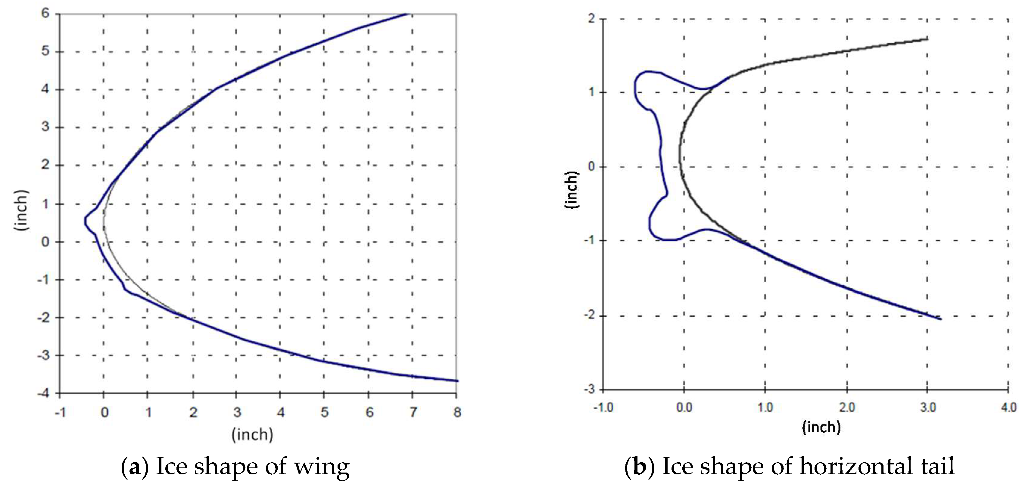
The aerodynamic parameters of the wing and horizontal tail: $C_{Z\alpha W}$, $C_{Z\alpha H}$, $C_{Z\delta eH}$ are calculated under both clean and iced conditions with the ice shapes of the wings and horizontal tail chosen from [17] by the individual component CFD method. As an illustration, Figure 9 shows the grid for CFD calculation of the horizontal tail. The calculation conditions are based on the icing flight test conditions: flight speed $V_{\infty }$ = 55 m/s, flight altitude H = 1200 m.

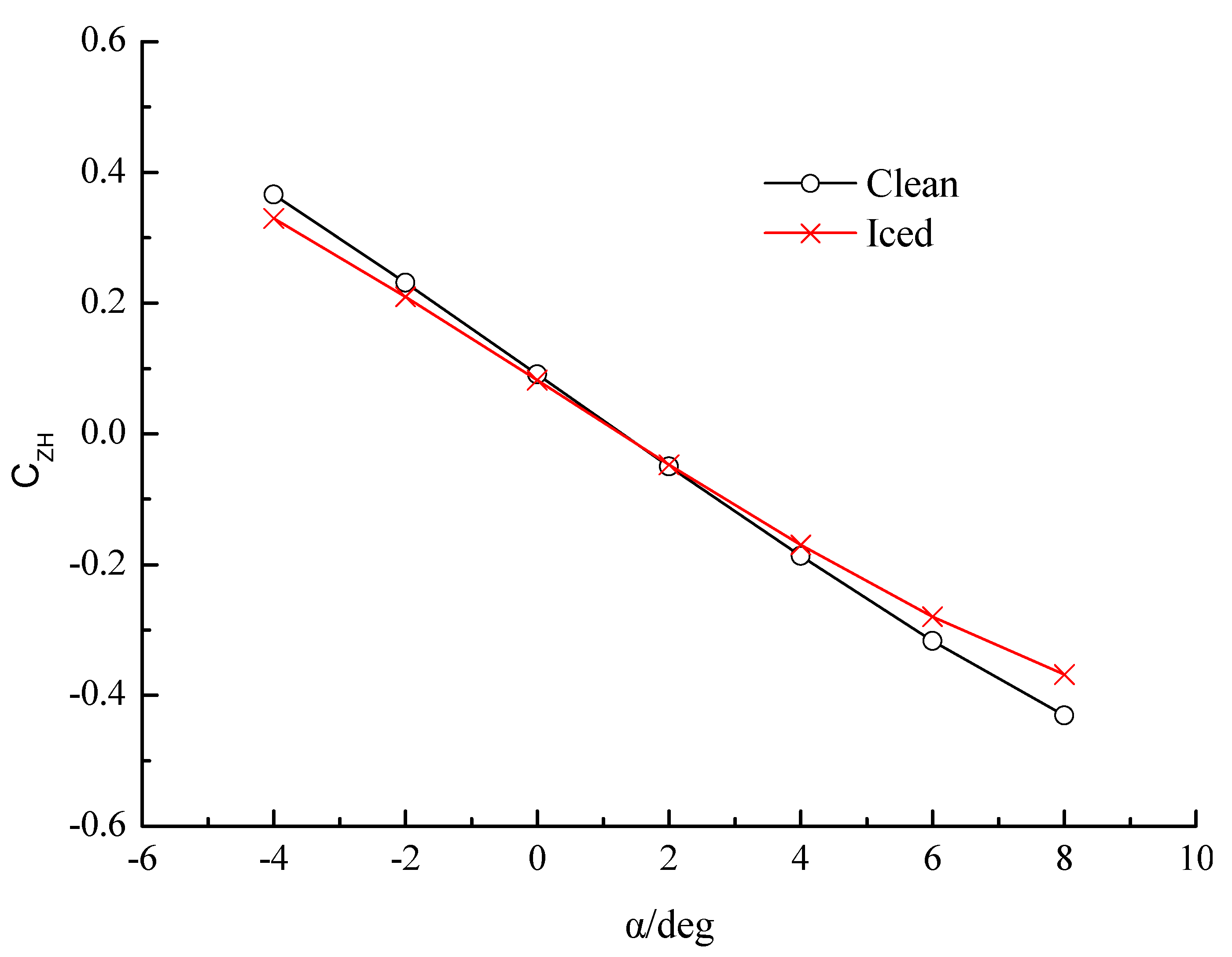
According to the calculation results, the curves of $C_{ZH}$ with angle of attack are drawn, as shown in Figure 10. The slope obtained by linear fitting the two curves can be used as the estimated value of $C_{ZH}$. The other parameters are calculated in the same way.

The results are shown in

Table 9. Aerodynamic derivatives of the wings and horizontal tail.

Aerodynamic Parameters	Clean	Iced
$C_{Z\alpha W}$	−4.772	−4.461
$C_{Z\alpha H}$	−3.801	−3.330
$C_{Z\delta eH}$	−2.857	−2.384

. Additionally, the values of $C_{zqW}$ and $C_{zqH}$ can be calculated from Equation (19).

The value of differences between iced and clean aircraft aerodynamic parameters can be obtained by replacing the corresponding terms in Equations (16) and (18) with the above-calculated results. Then the aerodynamic parameters of iced aircraft are obtained by adding the differences to the aerodynamic parameters of clean aircraft identified in Section 4.1. The results are compared with the identification results of iced aircraft in Section 4.2 as shown in

Table 10. Comparison of different kinds of results.

Aerodynamic Parameters	Identification Results		Iced Aircraft Calculation Result	Errors between Iced and Identification Result
	Clean Aircraft	Iced Aircraft
$C_{Z\alpha }$	−5.640	−5.294	−5.219	−1.42
$C_{Zq}$	−15.75	−13.85	−14.90	7.58
$C_{Z\delta e}$	−0.812	−0.606	−0.702	15.84
$C_{m\alpha }$	−1.446	−1.008	−0.971	−3.67
$C_{mq}$	−29.50	−25.35	−26.25	3.55
$C_{m\delta e}$	−2.095	−1.621	−1.650	1.79

.

As shown in Table 10, the change tendency of the prediction results is coincident with the identification results. For several aerodynamic derivatives of iced aircraft, the error between calculation results and identification results is basically within 10%. Only $C_{Z\delta e}$ reaches 15.84%. These errors may be caused by some assumptions or simplifications used in the prediction method. For the dynamic derivative $C_{mq}$, which represents the pitch damping, the error 3.55% is not very large. Thus, the feasibility of the prediction method in estimating the longitudinal dynamic derivatives of iced aircraft is verified. Based on these validations, the prediction method with the coupled ‘strip’ technique and CFD calculation shows good agreement with the experiment, and it could be used to calculate the effects of icing on the aircraft longitudinal characteristics. With this prediction method, only the aircraft basic configuration, the clean aircraft longitudinal aerodynamic derivatives and the ice shape are needed to calculate the longitudinal aerodynamic derivatives of the iced aircraft. Therefore, this method has a wide range of application.

6. Conclusions

In this paper, a nonlinear longitudinal flight dynamics model of rigid aircraft is established. For the aircraft with flight test, based on the maximum likelihood criterion, the identification system of aircraft aerodynamic parameters is established. For the aircraft without a flight test, based on the individual component CFD calculation and narrow strip theory, an engineering prediction method of longitudinal aerodynamic derivatives is established. According to NASA’s icing flight test data, longitudinal aerodynamic parameters of clean and icing aircraft in different conditions were identified. The aerodynamic parameters of the same icing aircraft are also calculated by the engineering prediction method. The difference between the results of the two methods and the reference value is compared, and the correctness of the two methods is verified. Through the above research and analysis, we can draw the following conclusions:

(1)

The aerodynamic parameters identification system based on the maximum likelihood criterion can predict the longitudinal aerodynamic parameters of iced aircraft relatively accurately. Through the analysis and verification of several examples, the method is practical.

(2)

The engineering prediction method established in this paper shows good agreement with the experiment. On the basis of known aircraft configuration and ice shape, this method can be used to calculate the effect of icing on the aircraft longitudinal aerodynamic parameters.

(3)

Icing has many adverse effects on aircraft flight, such as reduced lift, increased drag and reduced elevator effectiveness. The main wing icing plays a leading role in the change of aircraft lift and drag characteristics under icing conditions.

References

1. Whalen, E.; Bragg, M.B. Aircraft characterization in icing using flight test data. J. Aircr. 2005, 42, 792–794. [Google Scholar] [CrossRef]
2. Authority, C.A. Aircraft Icing Handbook; Safety Education and Publishing Unit: Lower Hutt, New Zealand, 2000. [Google Scholar]
3. Cao, Y.; Tan, W.; Wu, Z. Aircraft icing: An ongoing threat to aviation safety. Aerosp. Sci. Technol. 2018, 75, 353–385. [Google Scholar] [CrossRef]
4. Ranaudo, R.J.; Mikkelsen, K.L.; McKnight, R.C. The Measurement of Aircraft Performance and Stability and Control after Flight through Natural Icing Conditions; National Aeronautics and Space Administration: Washington, DC, USA, 1986.
5. Ratvasky, T.P.; Ranaudo, R.J. Icing Effects on Aircraft Stability and Control Determined from Flight Data; National Aeronautics and Space Administration: Washington, DC, USA, 1993.
6. Whalen, E.; Lee, S.; Bragg, M. Characterizing the Effect of Ice on Aircraft Performance and Control from flight data. AIAA Pap. 2002, 816, 2002. [Google Scholar]
7. Morelli, E. Multiple input design for real-time parameter estimation in the frequency domain. IFAC Proc. 2003, 36, 639–644. [Google Scholar] [CrossRef] [Green Version]
8. Melody, J.W.; Başar, T.; Perkins, W.R. Parameter identification for inflight detection and characterization of aircraft icing. Control Eng. Pract. 2000, 8, 985–1001. [Google Scholar] [CrossRef]
9. Ranaudo, R.J.; Reehorst, A.L.; Bond, T.H. Determination of longitudinal aerodynamic derivatives using flight data from an icing research aircraft. In Proceedings of the 27th Aerospace Sciences Meeting, Reno, NV, USA, 9–12 January 1989; p. 754. [Google Scholar]
10. Bragg, M.; Hutchison, T.; Merret, J. Effect of ice accretion on aircraft flight dynamics. In Proceedings of the 38th Aerospace Sciences Meeting and Exhibit, Reno, NV, USA, 10–13 January 2000; p. 360. [Google Scholar]
11. Lampton, A.; Valasek, J. Prediction of icing effects on the lateral/directional stability and control of light airplanes. Aerosp. Sci. Technol. 2012, 23, 305–311. [Google Scholar] [CrossRef]
12. Ratvasky, T.; Van Zante, J.; Riley, J. NASA/FAA tailplane icing program overview. In Proceedings of the 37th Aerospace Sciences Meeting and Exhibit, Reno, NV, USA, 11–14 January 1999; p. 370. [Google Scholar]
13. Hiltner, D.; McKee, M.; LaNoe, K. DHC-6 Twin Otter Tailplane Airfoil Section Testing in the Ohio State University 7x10 Wind Tunnel; National Aeronautics and Space Administration: Washington, DC, USA, 2000; Volume 1.
14. Di Donato, P.; Yoneyama, T.; Macau, E. Airplane Ice Accretion Detection Using Parameter Estimation. In Proceedings of the AIAA Guidance, Navigation, and Control Conference, Minneapolis, MN, USA, 13–16 August 2012; p. 4890. [Google Scholar]
15. Ratvasky, T.P.; Barnhart, B.P.; Lee, S. Current methods modeling and simulating icing effects on aircraft performance, stability, control. J. Aircr. 2010, 47, 201–211. [Google Scholar] [CrossRef]
16. Deiler, C. Aerodynamic modeling, system identification, and analysis of iced aircraft configurations. J. Aircr. 2018, 55, 145–161. [Google Scholar] [CrossRef]
17. Ratvasky, T.P.; Blankenship, K.; Rieke, W. Iced Aircraft Flight Data for Flight Simulator Validation. SAE Trans. 2002, 111, 100–112. [Google Scholar]
18. Ratvasky, T.P.; Van Zante, J.F.; Sim, A. NASA/FAA Tailplane Icing Program: Flight Test Report; National Aeronautics and Space Administration: Washington, DC, USA, 2000.
19. Taylor, L.W.; Iliff, K.W. Systems Identification Using a Modified Newton-Raphson Method: A FORTRAN Program; National Aeronautics and Space Administratration: Washington, DC, USA, 1972.
20. Wolowicz, C.H.; Yancey, R.B. Longitudinal Aerodynamic Characteristics of Light, Twin-Engine, Propeller-Driven Airplanes; NASA: Washington, DC, USA, 1972.
21. Wykes, J.H.; Casteel, G.R.; Collins, R.A. An Analytical Study of the Dynamics of Spinning Aircraft; Wright Air Development Center: Dayton, OH, USA, 1958; pp. 58–381.
22. Etkin, B.; Reid, L.D. Dynamics of Flight: Stability and Control; Wiley: New York, NY, USA, 1996; pp. 98–100. [Google Scholar]
Figure 1. Coordinate systems of longitudinal motion of aircraft.
Mathematics 08 01171 g001
Figure 2. Procedure of the identification program.
Mathematics 08 01171 g002
Figure 3. Output responses for the model validation.
Mathematics 08 01171 g003
Figure 4. Output responses of clean aircraft.
Mathematics 08 01171 g004aMathematics 08 01171 g004b
Figure 5. Ice shape of horizontal tail [18].
Mathematics 08 01171 g005
Figure 6. Angle of attack responses of horizontal tail iced aircraft.
Mathematics 08 01171 g006aMathematics 08 01171 g006b
Figure 7. Ice shape of “all iced” aircraft [17].
Mathematics 08 01171 g007
Figure 8. Output Responses of “all iced” Aircraft.
Mathematics 08 01171 g008aMathematics 08 01171 g008b
Figure 9. The grid of horizontal tail.
Mathematics 08 01171 g009
Figure 10. The curves of C Z H with angle of attack.
Mathematics 08 01171 g010