The Size-Dependent Thermoelastic Vibrations of Nanobeams Subjected to Harmonic Excitation and Rectified Sine Wave Heating

Abstract

In this article, a nonlocal thermoelastic model that illustrates the vibrations of nanobeams is introduced. Based on the nonlocal elasticity theory proposed by Eringen and generalized thermoelasticity, the equations that govern the nonlocal nanobeams are derived. The structure of the nanobeam is under a harmonic external force and temperature change in the form of rectified sine wave heating. The nonlocal model includes the nonlocal parameter (length-scale) that can have the effect of the small-scale. Utilizing the technique of Laplace transform, the analytical expressions for the studied fields are reached. The effects of angular frequency and nonlocal parameters, as well as the external excitation on the response of the nanobeam are carefully examined. It is found that length-scale and external force have significant effects on the variation of the distributions of the physical variables. Some of the obtained numerical results are compared with the known literature, in which they are well proven. It is hoped that the obtained results will be valuable in micro/nano electro-mechanical systems, especially in the manufacture and design of actuators and electro-elastic sensors.

1. Introduction

In recent decades, due to the rapid advancement in engineering technology and stringent training requirements, dynamics and stability and their control over mechanical vibration have gradually transformed into a fundamental and indivisible branch of study in applied mechanics and related engineering. Mechanical vibration is considered in many conditions and circumstances as a useful phenomenon, used in many areas and can also better serve people’s lives. Vibration analysis is fundamental for developments, as well as structural and mechanical system design. These data support us to predict the performance of the structure under various external loads and to design a control system, which is used to analyze the development vibrations in a cantilever beam instead of the structure itself [1].

The field of micro-electro-mechanical systems (MEMSs) is fast becoming involved in many resistance and correspondence applications. Modern technologies have been created to manufacture a variety of MEMS gadgets to meet the demand for many precision industries. MEMSs consist of elastic mechanical parts, such as micro-bridges, cantilevers, and microscopic films of various geometrical sizes and engineering forms that often contain loads [2]. It is imperative for MEMS designers to understand the mechanical properties of elastic micro-components, considering the ultimate goal of predicting the amount of deflection from the applied load and the additional method of avoiding cracking, performance development, and increasing the shelf life of MEMS devices [3].

Because of its applicability to a variety of problems, MEMSs have been applied in the fields of engineering applications and mathematical physics, including numerical methods and theoretical studies [4,5,6,7,8,9,10,11]. Advanced apparatuses created on the basis of resonators, modern science, microscale switches, telephones, mirrors, and pumps are cases of this approach [12,13].

Both investigations and atomic reproduction calculations have established an important dimension influence in the properties of mechanical materials when the sizes of these engineering structures are very small. As a result, the scale effect plays a principal role in the dynamic and static behavior of materials and micro/nanostructures and cannot be slighted. It is also known that classical mechanics do not represent such dimensional influences in small-scale and nano-scale structures.

The fundamental distinction between the classical theory of elasticity and the nonlocal Eringen theory [14] depends on the meaning of stress. In the local elasticity theory, stress at a point is a function of strain only at that point, while in the nonlocal elasticity theory, the stress at any point is an element of the strains at all points in the continuum. In the theory of local resilience, stress at a point is a function of motion at that point, while in non-local elasticity, stress at any point is an element of strains at all points in the continuum. Thus, the theory of nonlocal elasticity includes information about long-range powers around atoms, and therefore the length of the internal scale is taken into account. However, the nonlocal theory has been connected to different fields of physics, containing the lattice distribution of the elastic and thermoelastic waves, the dislocation mechanism [15], etc.

The dynamical interaction of solid and strong materials that are subjected to load movement is one of strong building and engineering areas, for instance, sea industrial, structural designing, earthquake design, and tribal science. For example, ground motion and stresses are prompted in submerged soils by rapidly moving vehicular loads or surface influence waves due to explosives. Many researchers have considered the dynamic interaction of beams and rods under moving forces. To consider the thermoelastic behavior of the structure caused by a harmonic external force, it is important to obtain the temperature distribution first [16,17,18,19,20,21,22,23,24].

All the studies mentioned above do not involve varying temperatures. Elastic bodies, as well as microbeams, are often in actual engineering applications under a variable temperature environment, so the variable temperature must be taken into account. The generalized thermoelasticity theories consider the influence of the coupling between the temperature and the rate of the strain. In addition, the resulting associated equations are of the hyperbolic type. Consequently, the discrepancy with respect to the infinite velocity of the spread of thermal waves in the classical coupled theory is disregarded. One of the most famous theories of generalized thermoelasticity that we will use in this work is Lord and Shulman's theory [25] that includes the time of thermal relaxation.

The free transversal vibrations of a complex system of coupled nanobeams attracted much attention in the scientific community. Few researchers have linked the theory of thermoelasticity to mechanical vibrations within nanomaterials. Many of them take the effect of the temperature in the form of a thermal load only, similar to the initial stress, and impose the thermal distribution in a specific way. They obtain the temperature distribution by solving the steady-state heat conduction equation with boundary conditions on the lower and upper surfaces of the nanobeam across the thickness.

According to the best knowledge of the authors, this is only one of a few studies that combine the system coupled with elastic nanobeams and generalized thermoelasticity (non-Fourier conduction equation). In addition to what was mentioned, in this paper, we obtained analytical solutions for different physical distributions using Laplace transforms without the need to impose the form of solutions, whether a harmonic solution or otherwise. In addition, the proposed model and methodology introduced in this work can be applied to study and describe the thermodynamic behavior of axial nanomaterial systems, such as nanoplates or nanoscale rods with thermoelastic properties.

In this investigation, the thermoelastic nonlocal theory is applied to the Euler Bernoulli beam problem subjected to a dispersed harmonic excitation load per unit length. The non-Fourier conduction equation depends on the thermal relaxation times [25] that are applied. The Laplace transform procedure is utilized as part of the deduction. The effects due to the harmonic external load, nonlocal and angular frequency parameters are represented graphically and are investigated. The current model can be used in micro/nano-electro-mechanical applications, such as mass flow sensors, accelerometers, relay switches, frequency filters and resonators. The vibration of nanobeams is a significant topic for the study of nanotechnology, as it relates to the optical and electronic properties of the nanobeams.

2. Theoretical Problem Formulations

The schematic representation of the considered system is illustrated in Figure 1, showing a hinged–hinged nanobeam of length $\mathrm{L}$ $\left(0\le \mathrm{x}\le \mathrm{L}\right)$, width $\mathrm{b}$ $\left(-\mathrm{b}/2\le \mathrm{y}\le \mathrm{b}/2\right)$ and thickness $\mathrm{h}$ $\left(-\mathrm{h}/2\le \mathrm{z}\le \mathrm{h}/2\right)$ and Young’s modulus $\mathrm{E}$, assuming that the Euler–Bernoulli beam theory is employed for modeling the nanobeams and the cross section of the nanobeam is uniform along the entire length. Hence, the displacements of the beam can be written as

$$\mathrm{u}=-\mathrm{z}\frac{\partial \mathrm{w}}{\partial \mathrm{x}},\mathrm{v}=0,\mathrm{w}=\mathrm{w}\left(\mathrm{x},\mathrm{t}\right),$$

(1)

where $\mathrm{w}\left(\mathrm{x},\mathrm{t}\right)$ denotes the transverse displacement (lateral deflection) of the nanobeam.

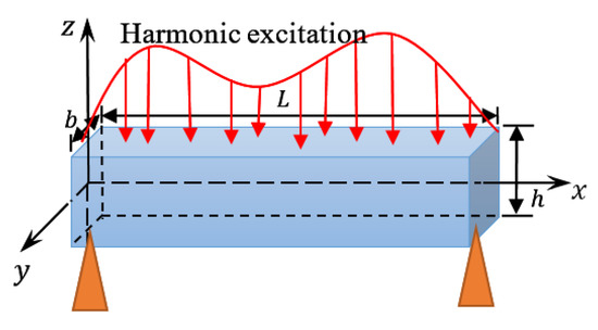
Figure 1. Schematic diagram for the nanobeam.

Based on Eringen’s nonlocal elasticity theory [14,15], the constitutive relation for a one-dimensional problem, after using Equation (11), can be written as

$${\mathsf{\sigma }}_{\mathrm{x}}-\mathsf{\xi }\frac{{\partial }^2{\mathsf{\sigma }}_{\mathrm{x}}}{\partial {\mathrm{x}}^2}=-\mathrm{E}\left(\mathrm{z}\frac{{\partial }^2\mathrm{w}}{\partial {\mathrm{x}}^2}+{\mathsf{\alpha }}_{\mathrm{T}}\mathsf{\theta }\right),$$

(2)

where ${\mathsf{\sigma }}_{\mathrm{x}}$ is the nonlocal axial stress, $\mathsf{\theta }=\mathrm{T}-{\mathrm{T}}_0$ is the resonator temperature change, $\mathrm{T}$ is the distribution of temperature and ${\mathrm{T}}_0$ denotes the environmental temperature, ${\mathsf{\alpha }}_{\mathrm{T}}={\mathsf{\alpha }}_{\mathrm{t}}/\left(1-2\mathsf{\nu }\right)$, $\mathsf{\nu }$ is Poisson’s ratio and ${\mathsf{\alpha }}_{\mathrm{t}}$ is the linear thermal expansion.

In Equation (2), the nonlocal parameter is $\mathsf{\xi }={\left({\mathrm{e}}_{0}a\right)}^2$, where $a$ is the internal characteristic length and ${\mathrm{e}}_0$ is a suitable parameter that can be determined by the experiment. When the characteristic parameter $a$ is neglected, then $\mathsf{\xi }=0$, and Equation (2) reduces to the classical constitutive relation (local elasticity).

The bending moment $\mathrm{M}\left(\mathrm{x},\mathrm{t}\right)$ is given by

$$\mathrm{M}\left(\mathrm{x},\mathrm{t}\right)={{\displaystyle \int }}_{-\mathrm{h}/2}^{\mathrm{h}/2}{\mathrm{z}\mathsf{\sigma }}_{\mathrm{x}}\mathrm{dz}.$$

(3)

Substitution of Equation (2) into Equation (3) results in

$$\mathrm{M}\left(\mathrm{x},\mathrm{t}\right)-\mathsf{\xi }\frac{{\partial }^2\mathrm{M}}{\partial {\mathrm{x}}^2}=-\mathrm{EI}\left(\frac{{\partial }^2\mathrm{w}}{\partial {\mathrm{x}}^2}+{\mathsf{\alpha }}_{\mathrm{T}}{\mathrm{M}}_{\mathrm{T}}\right)$$

(4)

where $\mathrm{I}={\mathrm{bh}}^3/12$ and ${\mathrm{M}}_{\mathrm{T}}$ is the thermal moment defined by

$${\mathrm{M}}_{\mathrm{T}}=\frac{12}{{\mathrm{h}}^3}{{\displaystyle \int }}_{-\mathrm{h}/2}^{\mathrm{h}/2}\mathsf{\theta }\left(\mathrm{x},\mathrm{z},\mathrm{t}\right)\mathrm{zdz}$$

(5)

When the beam is due to a distributed load $\mathrm{q}\left(\mathrm{x},\mathrm{t}\right)$, the transverse motion equation is as follows [24]:

$$\frac{{\partial }^2\mathrm{M}}{\partial {\mathrm{x}}^2}=-\mathrm{q}\left(\mathrm{x},\mathrm{t}\right)+\mathsf{\rho }\mathrm{A}\frac{{\partial }^2\mathrm{w}}{\partial {\mathrm{t}}^2}.$$

(6)

where $\mathsf{\rho }$ is the density of the material and $\mathrm{A}$ is the cross section of the nanobeam.

Substitution of Equation (4) into Equation (6) results in

$$\mathrm{M}\left(\mathrm{x},\mathrm{t}\right)=\mathsf{\xi }\left(\mathsf{\rho }\mathrm{A}\frac{{\partial }^2\mathrm{w}}{\partial {\mathrm{t}}^2}-\mathrm{q}\right)-\mathrm{EI}\left(\frac{{\partial }^2\mathrm{w}}{\partial {\mathrm{x}}^2}+{\mathsf{\alpha }}_{\mathrm{T}}{\mathrm{M}}_{\mathrm{T}}\right).$$

(7)

Substituting Equation (7) into Equation (6), Equation (6) can be rewritten in the form

$$\left[\frac{{\partial }^4}{\partial {\mathrm{x}}^4}+\frac{\mathsf{\rho }\mathrm{A}}{\mathrm{EI}}\frac{{\partial }^2}{\partial {\mathrm{t}}^2}\left(1-\mathsf{\xi }\frac{{\partial }^2}{\partial {\mathrm{x}}^2}\right)\right]\mathrm{w}-\frac{1}{\mathrm{EI}}\left(1-\mathsf{\xi }\frac{{\partial }^2}{\partial {\mathrm{x}}^2}\right)\mathrm{q}+{\mathsf{\alpha }}_{\mathrm{T}}\frac{{\partial }^2{\mathrm{M}}_{\mathrm{T}}}{\partial {\mathrm{x}}^2}=0.$$

(8)

The non-Fourier heat transfer equation, considering the entropy balance proposed by Lord and Shulman [25], which includes the heat flux in addition to its time derivative, is given as

$${\left({\mathrm{K}\mathsf{\theta }}_{,\mathrm{i}}\right)}_{,\mathrm{i}}+\left(1+{\mathsf{\tau }}_0\frac{\partial }{\partial \mathrm{t}}\right)\left(\mathsf{\rho }\mathrm{Q}\right)=\left(1+{\mathsf{\tau }}_0\frac{\partial }{\partial \mathrm{t}}\right)\frac{\partial }{\partial \mathrm{t}}\left({\mathsf{\rho }\mathrm{C}}_{\mathrm{E}}\mathsf{\theta }+{\mathsf{\gamma }\mathrm{T}}_0\mathrm{e}\right).$$

(9)

where $\mathrm{K}$ is the coefficient of thermal conductivity, $\mathrm{Q}$ is the heat source, ${\mathrm{C}}_{\mathrm{E}}$ denotes the specific heat at constant strain, ${\mathsf{\tau }}_0$ is the relaxation time characteristic according to the Lord and Shulman theory and $\mathrm{e}=\frac{\partial \mathrm{u}}{\partial \mathrm{x}}$ is the volumetric strain. Substituting Equation (1) into the heat equation, Equation (9), when$\mathrm{Q}=0$, is given by

$$\mathrm{K}\left(\frac{{\partial }^2}{\partial {\mathrm{x}}^2}+\frac{{\partial }^2}{\partial {\mathrm{z}}^2}\right)\mathsf{\theta }=\left(1+{\mathsf{\tau }}_0\frac{\partial }{\partial \mathrm{t}}\right)\frac{\partial }{\partial \mathrm{t}}\left({\mathsf{\rho }\mathrm{C}}_{\mathrm{E}}\mathsf{\theta }-{\mathsf{\gamma }\mathrm{T}}_0\mathrm{z}\frac{{\partial }^2\mathrm{w}}{\partial {\mathrm{x}}^2}\right)$$

(10)

3. Solution of the Problem

We assume that the increment of temperature change is in terms of a sine function (sinusoidal variation) as

$$\mathsf{\theta }\left(\mathrm{x},\mathrm{z},\mathrm{t}\right)=\mathsf{\Theta }\left(\mathrm{x},\mathrm{t}\right)\sin \left(\frac{\mathsf{\pi }}{\mathrm{h}}\mathrm{z}\right)$$

(11)

Using relation (11) in the governing Equations (7), (8) and (10), we obtain

$$\left[\frac{{\partial }^4}{\partial {\mathrm{x}}^4}+\frac{\mathsf{\rho }\mathrm{A}}{\mathrm{EI}}\frac{{\partial }^2}{\partial {\mathrm{t}}^2}\left(1-\mathsf{\xi }\frac{{\partial }^2}{\partial {\mathrm{x}}^2}\right)\right]\mathrm{w}-\frac{1}{\mathrm{EI}}\left(1-\mathsf{\xi }\frac{{\partial }^2}{\partial {\mathrm{x}}^2}\right)\mathrm{q}+\frac{24{\mathsf{\alpha }}_{\mathrm{T}}}{{\mathsf{\pi }}^2\mathrm{h}}\frac{{\partial }^2\mathsf{\Theta }}{\partial {\mathrm{x}}^2}=0,$$

(12)

$$\mathrm{M}\left(\mathrm{x},\mathrm{t}\right)=\mathsf{\xi }\left(\mathsf{\rho }\mathrm{A}\frac{{\partial }^2\mathrm{w}}{\partial {\mathrm{t}}^2}-\mathrm{q}\right)-\mathrm{EI}\left(\frac{{\partial }^2\mathrm{w}}{\partial {\mathrm{x}}^2}+\frac{24{\mathrm{T}}_0{\mathsf{\alpha }}_{\mathrm{T}}}{{\mathsf{\pi }}^2\mathrm{h}}\mathsf{\Theta }\right),$$

(13)

$$\left(1+{\mathsf{\tau }}_{\mathsf{\theta }}\frac{\partial }{\partial \mathrm{t}}\right)\left(\frac{{\partial }^2\mathsf{\Theta }}{\partial {\mathrm{x}}^2}-\frac{{\mathsf{\pi }}^2}{{\mathrm{h}}^2}\mathsf{\Theta }\right)=\left(1+{\mathsf{\tau }}_{\mathrm{q}}\frac{\partial }{\partial \mathrm{t}}\right)\frac{\partial }{\partial \mathrm{t}}\left(\frac{{\mathsf{\rho }\mathrm{C}}_{\mathrm{E}}}{\mathrm{K}}\mathsf{\Theta }-\frac{{\mathsf{\gamma }\mathrm{T}}_0{\mathsf{\pi }}^2\mathrm{h}}{24\mathrm{K}}\frac{{\partial }^2\mathrm{w}}{\partial {\mathrm{x}}^2}\right).$$

(14)

Introducing the following non-dimensional quantities:

$$\begin{gathered} \left\{{\mathrm{x}}^{\prime },{\mathrm{w}}^{\prime },{\mathrm{u}}^{\prime },{\mathrm{z}}^{\prime },{\mathrm{L}}^{\prime },{\mathrm{h}}^{\prime },{\mathrm{b}}^{\prime }\right\} = \mathsf{\eta }\mathrm{c}\left\{\mathrm{x},\mathrm{w},\mathrm{u},\mathrm{z},\mathrm{L},\mathrm{h},\mathrm{b}\right\},\hspace{1em}\left\{{\mathrm{t}}^{\prime },{\mathsf{\tau }}_{\mathrm{q}}^{\prime },{\mathsf{\tau }}_{\mathsf{\theta }}^{\prime }\right\} = {\mathsf{\eta }\mathrm{c}}^2\left\{t,{\mathsf{\tau }}_{\mathrm{q}},{\mathsf{\tau }}_{\mathsf{\theta }}\right\}, \\ {\mathsf{\Theta }}^{\prime } = \frac{1}{{\mathrm{T}}_0}\mathsf{\Theta },\hspace{1em}{\mathsf{\xi }}^{\prime } = {\mathsf{\eta }}^2{\mathrm{c}}^2\mathsf{\xi },\hspace{1em}{\mathrm{M}}^{\prime } = \frac{1}{\mathsf{\eta }\mathrm{cEI}}\mathrm{M}, {\mathrm{q}}^{\prime } = \frac{\mathrm{A}}{\mathrm{EI}}\mathrm{q},\hspace{1em}{\mathrm{c}}^2 = \frac{\mathrm{E}}{\mathsf{\rho }},\hspace{1em}\mathsf{\eta }=\frac{\mathsf{\rho }{\mathrm{C}}_{\mathrm{E}}}{\mathrm{K}} \end{gathered}$$

(15)

Substitution of (15) into (12)–(14) results in (dropping the primes for convenience)

$$\left[\frac{{\partial }^4}{\partial {\mathrm{x}}^4}+\frac{12}{{\mathrm{h}}^2}\frac{{\partial }^2}{\partial {\mathrm{t}}^2}\left(1-\mathsf{\xi }\frac{{\partial }^2}{\partial {\mathrm{x}}^2}\right)\right]\mathrm{w}-\left(1-\mathsf{\xi }\frac{{\partial }^2}{\partial {\mathrm{x}}^2}\right)\mathrm{q}+\frac{24{\mathrm{T}}_0{\mathsf{\alpha }}_{\mathrm{T}}}{{\mathsf{\pi }}^2\mathrm{h}}\frac{{\partial }^2\mathsf{\Theta }}{\partial {\mathrm{x}}^2}=0,$$

(16)

$$\frac{{\partial }^2\mathsf{\Theta }}{\partial {\mathrm{x}}^2}-\frac{{\mathsf{\pi }}^2}{{\mathrm{h}}^2}\mathsf{\Theta }=\left(1+{\mathsf{\tau }}_0\frac{\partial }{\partial \mathrm{t}}\right)\frac{\partial }{\partial \mathrm{t}}\left(\mathsf{\Theta }-\frac{{\mathsf{\gamma }\mathsf{\pi }}^2\mathrm{h}}{24\mathrm{K}\mathsf{\eta }}\frac{{\partial }^2\mathrm{w}}{\partial {\mathrm{x}}^2}\right),$$

(17)

$$\mathrm{M}\left(\mathrm{x},\mathrm{t}\right)=\frac{12\mathsf{\xi }}{{\mathrm{h}}^2}\frac{{\partial }^2\mathrm{w}}{\partial {\mathrm{t}}^2}-\mathsf{\xi }\mathrm{q}\left(\mathrm{x}\right)-\frac{{\partial }^2\mathrm{w}}{\partial {\mathrm{x}}^2}-\frac{24{\mathrm{T}}_0{\mathsf{\alpha }}_{\mathrm{T}}}{{\mathsf{\pi }}^2\mathrm{h}}\mathsf{\Theta }$$

(18)

In general, the harmonic excitation $\mathrm{q}\left(\mathrm{x},\mathrm{t}\right)$ has the form of a sine or cosine function of a single frequency. In this problem, the dynamic load $\mathrm{q}\left(\mathrm{x},\mathrm{t}\right)$ can be considered as

$$\mathrm{q}\left(\mathrm{x},\mathrm{t}\right)={\mathrm{F}}_0\cos \left(\mathsf{\Omega }\mathrm{t}\right),$$

(19)

where ${\mathrm{F}}_0$ is the magnitude of forcing excitation and $\mathsf{\Omega }$ is the frequency of the external excitations ($\mathsf{\Omega }=0$ for the uniformly distributed load).

4. Boundary Conditions

Let us also consider what the boundary conditions are assumed to be, as in Table 1

Table 1. The boundary conditions of the problem.

x	Mechanical Boundary Conditions	Thermal Boundary Conditions
$\mathrm{x}=0$	$\mathrm{w}\left(\mathrm{x},\mathrm{t}\right)=0$, $\frac{{\partial }^2\mathrm{w}\left(\mathrm{x},\mathrm{t}\right)}{\partial {\mathrm{x}}^2}=0$	$\mathsf{\theta }=\mathsf{\theta }\left(\mathrm{x},\mathrm{z},\mathrm{t}\right)=\sin \left(\mathrm{pz}\right)\mathrm{f}\left(\mathrm{x},\mathrm{t}\right)$
$\mathrm{x}=\mathrm{L}$	$\mathrm{w}\left(\mathrm{x},\mathrm{t}\right)=0$, $\frac{{\partial }^2\mathrm{w}\left(\mathrm{x},\mathrm{t}\right)}{\partial {\mathrm{x}}^2}=0$	$\mathrm{K}\frac{\partial \mathsf{\theta }}{\partial \mathrm{x}}=0$

In Table 1, the function $\mathrm{f}\left(\mathrm{x},\mathrm{t}\right)$ is a varying rectified sine wave function which is described mathematically as

$$\mathrm{f}\left(\mathrm{x},\mathrm{t}\right)={\mathsf{\Theta }}_0\left|\sin \left(\mathsf{\omega }\mathrm{t}\right)\right|,$$

(20)

where ${\mathsf{\Theta }}_0$ is a constant and $\mathsf{\omega }$ is the frequency of the rectified sine wave.

5. Solution in the Transformed Space

In this problem, the initial conditions are assumed to be

$${\mathrm{w}\left(\mathrm{x},\mathrm{t}\right)|}_{\mathrm{t}=0}={\frac{\partial \mathrm{w}\left(\mathrm{x},\mathrm{t}\right)}{\partial \mathrm{t}}|}_{\mathrm{t}=0}=0,{\mathsf{\Theta }\left(\mathrm{x},\mathrm{t}\right)|}_{\mathrm{t}=0}={\frac{\partial \mathsf{\Theta }\left(\mathrm{x},\mathrm{t}\right)}{\partial \mathrm{t}}|}_{\mathrm{t}=0}=0.$$

(21)

Employing the technique of Laplace transform to Equations (16)–(18), we obtain

$$\left[\frac{{\mathrm{d}}^4}{{\mathrm{dx}}^4}-{\mathrm{A}}_3{\mathrm{s}}^2\frac{{\mathrm{d}}^2}{{\mathrm{dx}}^2}+{\mathrm{A}}_1{\mathrm{s}}^2\right]\overline{\mathrm{w}}=-{\mathrm{A}}_2\frac{{\mathrm{d}}^2\overline{\mathsf{\Theta }}}{{\mathrm{dx}}^2}+\overline{\mathrm{g}}\left(\mathrm{s}\right),$$

(22)

$$\left(\frac{{\mathrm{d}}^2}{{\mathrm{dx}}^2}-{\mathrm{B}}_1\right)\overline{\mathsf{\Theta }}=-{\mathrm{B}}_2\frac{{\mathrm{d}}^2\overline{\mathrm{w}}}{{\mathrm{dx}}^2},$$

(23)

$$\overline{\mathrm{M}}\left(\mathrm{x},\mathrm{s}\right)=-\left(\frac{{\mathrm{d}}^2}{{\mathrm{dx}}^2}-{\mathrm{A}}_3{\mathrm{s}}^2\right)\overline{\mathrm{w}}-{\mathrm{A}}_2\overline{\mathsf{\Theta }}-\mathsf{\xi }\overline{\mathrm{g}}\left(\mathrm{s}\right),$$

(24)

where

$$\begin{gathered} {\mathrm{A}}_1 = \frac{12}{{\mathrm{h}}^2},\hspace{1em}{\mathrm{A}}_2 = \frac{24{\mathrm{T}}_0{\mathsf{\alpha }}_{\mathrm{T}}}{{\mathsf{\pi }}^2\mathrm{h}},\hspace{1em}{\mathrm{A}}_3 = \mathsf{\xi }{\mathrm{A}}_1,\hspace{1em}{\mathrm{A}}_4 = \frac{{\mathsf{\pi }}^2}{{\mathrm{h}}^2},\hspace{1em}{\mathrm{A}}_5 = \frac{{\mathsf{\gamma }\mathsf{\pi }}^2\mathrm{h}}{24\mathrm{K}\mathsf{\eta }}, \\ {\mathrm{B}}_1 = {\mathrm{A}}_4 + \mathrm{s}\left(1+{\mathsf{\tau }}_0\mathrm{s}\right),\hspace{1em}{\mathrm{B}}_2 = \mathrm{s}\left(1+{\mathsf{\tau }}_0\mathrm{s}\right){\mathrm{A}}_5,\hspace{1em}\overline{\mathrm{g}}\left(\mathrm{s}\right) = \frac{{\mathrm{sF}}_0}{{\mathsf{\Omega }}^2+{\mathrm{s}}^2} \end{gathered}$$

(25)

From Equations (22) and (23), we can obtain

$$\left[\frac{{\mathrm{d}}^6}{{\mathrm{dx}}^6}-\mathrm{A}\frac{{\mathrm{d}}^4}{{\mathrm{dx}}^4}+\mathrm{B}\frac{{\mathrm{d}}^2}{{\mathrm{dx}}^2}-\mathrm{C}\right]\overline{\mathrm{w}}=0,$$

(26)

where

$$\mathrm{A}={\mathrm{B}}_1+{\mathrm{A}}_2{\mathrm{B}}_2+{\mathrm{A}}_3{\mathrm{s}}^2,\mathrm{B}={\mathrm{s}}^2\left({\mathrm{A}}_1+{\mathrm{A}}_3{\mathrm{B}}_1\right),\mathrm{C}={\mathrm{A}}_1{\mathrm{B}}_1{\mathrm{s}}^2.$$

(27)

The general solution to Equation (26) can be presented as:

$$\overline{\mathrm{w}}\left(\mathrm{x},\mathrm{s}\right)={\displaystyle \sum }_{\mathrm{j}=1}^3\left({\mathrm{L}}_{\mathrm{j}}\sinh ({\mathrm{m}}_{\mathrm{j}}\mathrm{x})+{\mathrm{M}}_{\mathrm{j}}\cosh ({\mathrm{m}}_{\mathrm{j}}\mathrm{x})\right),$$

(28)

where ${\mathrm{L}}_{\mathrm{j}}$ and ${\mathrm{M}}_{\mathrm{j}}$ are the integral parameters and $\pm {\mathrm{m}}_{\mathrm{j}},\left(\mathrm{j}=1,2,3\right)$ satisfy the equation

$${\mathrm{m}}^6-{\mathrm{Am}}^4+{\mathrm{Bm}}^2-\mathrm{C}=0.$$

(29)

From Equations (26) and (25), we can obtain

$$\overline{\mathsf{\Theta }}\left(\mathrm{x},\mathrm{s}\right)=-\frac{1}{{\mathrm{A}}_2{\mathrm{B}}_1}\left[\frac{{\mathrm{d}}^4\overline{\mathrm{w}}}{{\mathrm{dx}}^4}-\left({\mathrm{A}}_2{\mathrm{B}}_2+{\mathrm{A}}_3{\mathrm{s}}^2\right)\frac{{\mathrm{d}}^2\overline{\mathrm{w}}}{{\mathrm{dx}}^2}+{\mathrm{A}}_1{\mathrm{s}}^2\overline{\mathrm{w}}-\overline{\mathrm{g}}\left(\mathrm{s}\right)\right].$$

(30)

The general solutions of Equation (10) with the help of Equation (30) can be simplified as

$$\overline{\mathsf{\Theta }}\left(\mathrm{x},\mathrm{s}\right)={\displaystyle \sum }_{\mathrm{j}=1}^3{\mathrm{H}}_{\mathrm{j}}\left({\mathrm{L}}_{\mathrm{j}}\sinh ({\mathrm{m}}_{\mathrm{j}}\mathrm{x})+{\mathrm{M}}_{\mathrm{j}}\cosh ({\mathrm{m}}_{\mathrm{j}}\mathrm{x})\right)+{\mathrm{H}}_4,$$

(31)

where

$${\mathrm{H}}_{\mathrm{j}}=-\frac{1}{{\mathrm{A}}_2{\mathrm{B}}_1}\left[{\mathrm{m}}_{\mathrm{j}}^4-\left({\mathrm{A}}_2{\mathrm{B}}_2+{\mathrm{A}}_3{\mathrm{s}}^2\right){\mathrm{m}}_{\mathrm{j}}^2+{\mathrm{A}}_1{\mathrm{s}}^2\right],\mathrm{j}=1,2,3,{\mathrm{H}}_4=\frac{\overline{\mathrm{g}}\left(\mathrm{s}\right)}{{\mathrm{A}}_2{\mathrm{B}}_1}.$$

(32)

Introducing the solutions of $\overline{\mathrm{w}}$ and $\overline{\mathsf{\Theta }}$ into Equation (24) yields

$$\overline{\mathrm{M}}\left(\mathrm{x},\mathrm{s}\right)=-{\displaystyle \sum }_{\mathrm{j}=1}^3\left({\mathrm{m}}_{\mathrm{j}}^2-{\mathrm{A}}_3{\mathrm{s}}^2+{\mathrm{A}}_2{\mathrm{H}}_{\mathrm{j}}\right)\left({\mathrm{L}}_{\mathrm{j}}\sinh ({\mathrm{m}}_{\mathrm{j}}\mathrm{x})+{\mathrm{M}}_{\mathrm{j}}\cosh ({\mathrm{m}}_{\mathrm{j}}\mathrm{x})\right)-{\mathrm{A}}_2{\mathrm{H}}_4-\overline{\mathrm{g}}\left(\mathrm{s}\right)$$

(33)

The axial displacement $\overline{\mathrm{u}}$ is obtained using Equations (28) and (1) as

$$\overline{\mathrm{u}}=-\mathrm{z}\frac{\partial \overline{\mathrm{w}}}{\partial \mathrm{x}}=-\mathrm{z}{\displaystyle \sum }_{\mathrm{j}=1}^3{\mathrm{m}}_{\mathrm{j}}\left({\mathrm{L}}_{\mathrm{j}}\cosh ({\mathrm{m}}_{\mathrm{j}}\mathrm{x})+{\mathrm{M}}_{\mathrm{j}}\sinh ({\mathrm{m}}_{\mathrm{j}}\mathrm{x})\right).$$

(34)

Using the Laplace transform domain, the boundary conditions given in Table 1 may be written as

$${\overline{\mathrm{w}}\left(\mathrm{x},\mathrm{s}\right)|}_{\mathrm{x}=0,\mathrm{L}}=0,{\frac{{\mathrm{d}}^2\overline{\mathrm{w}}\left(\mathrm{x},\mathrm{s}\right)}{{\mathrm{dx}}^2}|}_{\mathrm{x}=0,\mathrm{L}}=0,$$

(35)

$${\overline{\mathsf{\Theta }}\left(\mathrm{x},\mathrm{s}\right)|}_{\mathrm{x}=0}={\mathsf{\Theta }}_0\left(\frac{\mathsf{\omega }\cosh \left(\frac{\mathsf{\pi }\mathrm{s}}{2\mathsf{\omega }}\right)}{{\mathsf{\omega }}^2+{\mathrm{s}}^2}\right)=\overline{\mathrm{G}}\left(\mathrm{s}\right),$$

(36)

$${\frac{\mathrm{d}\overline{\mathsf{\Theta }}}{\mathrm{dx}}|}_{\mathrm{x}=\mathrm{L}}=0.$$

(37)

Substituting (28) and (30) into Equations (35)–(37), one obtains

$${\displaystyle \sum }_{\mathrm{j}=1}^3{\mathrm{M}}_{\mathrm{j}}=0$$

(38)

$${\displaystyle \sum }_{\mathrm{j}=1}^3\left({\mathrm{L}}_{\mathrm{j}}\sinh ({\mathrm{m}}_{\mathrm{j}}\mathrm{L})+{\mathrm{M}}_{\mathrm{j}}\cosh ({\mathrm{m}}_{\mathrm{j}}\mathrm{L})\right)=0$$

(39)

$${\displaystyle \sum }_{\mathrm{j}=1}^3{\mathrm{m}}_{\mathrm{j}}^2{\mathrm{M}}_{\mathrm{j}}=0$$

(40)

$${\displaystyle \sum }_{\mathrm{j}=1}^3{\mathrm{m}}_{\mathrm{j}}^2\left({\mathrm{L}}_{\mathrm{j}}\sinh ({\mathrm{m}}_{\mathrm{j}}\mathrm{L})+{\mathrm{M}}_{\mathrm{j}}\cosh ({\mathrm{m}}_{\mathrm{j}}\mathrm{L})\right)=0$$

(41)

$${\displaystyle \sum }_{\mathrm{j}=1}^3{\mathrm{H}}_{\mathrm{j}}{\mathrm{M}}_{\mathrm{j}}+{\mathrm{H}}_4=\overline{\mathrm{G}}\left(\mathrm{s}\right)$$

(42)

$${\displaystyle \sum }_{\mathrm{j}=1}^3{\mathrm{H}}_{\mathrm{j}}\left({\mathrm{L}}_{\mathrm{j}}{\mathrm{m}}_{\mathrm{j}}\cosh ({\mathrm{m}}_{\mathrm{j}}\mathrm{x})+{\mathrm{M}}_{\mathrm{j}}{\mathrm{m}}_{\mathrm{j}}\sinh ({\mathrm{m}}_{\mathrm{j}}\mathrm{x})\right)=0$$

(43)

It is difficult to obtain direct Laplace transform inversion for the complicated solutions of the transformed studied fields. Thus, the physical solutions are obtained numerically using the Fourier expansion technique [26]. In this method, any function $\overline{\mathrm{g}}\left(\mathrm{x},\mathrm{s}\right)$ can be transformed to that in the domain of time $\mathrm{g}\left(\mathrm{x},\mathrm{t}\right)$ by the relation:

$$\mathrm{g}\left(\mathrm{x},\mathrm{t}\right)=\frac{{\mathrm{e}}^{\mathrm{ct}}}{\mathrm{t}}\left(\frac{1}{2}\overline{\mathrm{g}}\left(\mathrm{x},\mathrm{c}\right)+\mathrm{Re}{{\displaystyle \sum }}_{\mathrm{n}=1}^{{\mathrm{N}}_{\mathrm{f}}}\overline{\mathrm{g}}\left(\mathrm{x},\mathrm{c}+\frac{\mathrm{in}\mathsf{\pi }}{\mathrm{t}}\right){\left(-1\right)}^{\mathrm{n}}\right),$$

(44)

where ${\mathrm{N}}_{\mathrm{f}}$ is a finite number and the parameter $\mathrm{c}$ satisfies the relation $\mathrm{ct}\cong 4.7$ [27].

6. Numerical Results

The defined Tzou approximation technique [28] is employed to achieve the numerical results of the studied fields. The silicon (Si) material is selected for numerical calculation, and the physical constants at ${\mathrm{T}}_0=293\mathrm{K}$ are [23]:

$$\begin{array}{c}\mathrm{E}=169\mathrm{GPa},\mathsf{\rho }=2330\mathrm{kg}/{\mathrm{m}}^3,{\mathrm{C}}_{\mathrm{E}}=713\mathrm{J}/\left(\mathrm{kg}\mathrm{K}\right),\\ {\mathsf{\alpha }}_{\mathrm{T}}=2.59\times {10}^{-6}\left(1/\mathrm{K}\right),\mathsf{\nu }=0.22,\mathrm{K}=156\mathrm{W}/\left(\mathrm{mK}\right).\end{array}$$

In the calculation analysis, we take $\mathrm{L}/\mathrm{h}=10$ and $\mathrm{b}/\mathrm{h}=0.5$ and the parameter $\overline{\mathsf{\xi }}$ ($\overline{\mathsf{\xi }}={10}^2\mathsf{\xi }$) is also considered. The effects of several effective parameters on the conduct of the deflection of the nanobeam are explored. The numerical results are plotted in Figure 2, Figure 3 and Figure 4, which explain the variations of the distributions of lateral vibration, displacement, temperature and moment, concerning different parameters.

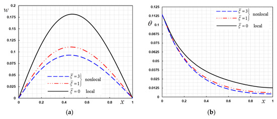
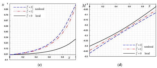
Figure 2. (a): The deflection $w$ for different values of the nonlocal parameter $\overline{\xi }$. (b): The temperature $\mathsf{\theta }$ for different values of the nonlocal parameter $\overline{\xi }$. (c): The displacement $\mathrm{u}$. for different values of the nonlocal parameter $\overline{\xi }$. (d): The distribution of bending moment $M$ for different values of the nonlocal parameter $\overline{\xi }$.

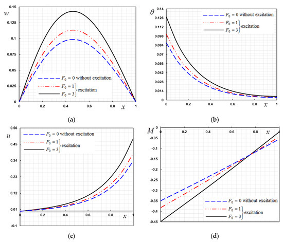
Figure 3. (a) The deflection $\mathrm{w}$ for different magnitudes of the forcing excitation F₀. (b): The temperature $\mathsf{\theta }$ for different magnitudes of the forcing excitation F₀ (c): The displacement $\mathrm{u}$ for different magnitudes of the forcing excitation F₀. (d): The bending moment $M$ for different magnitudes of the forcing excitation $F_0$

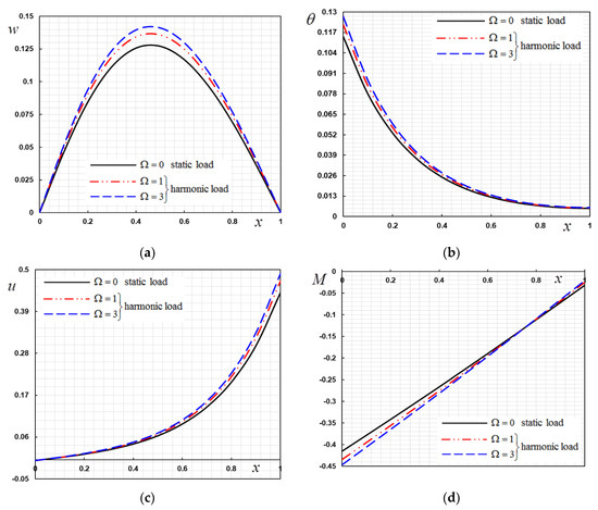
Figure 4. (a) The distribution of deflection w for different frequencies of the external excitation $\mathsf{\Omega }$ (b): The distribution of temperature $\mathsf{\theta }$ for different frequencies of the external excitation Ω. (c): The distribution of displacement $\mathrm{u}$ for different frequencies of the external excitation $\mathsf{\Omega }$. (d): The distribution of bending moment $M$ for different frequencies of the external excitation $\mathsf{\Omega }$.

Figure 2a–d illustrate the variety of the dimensionless studied fields of the system versus the distance $\mathrm{x}$ when $\mathrm{L}=1$, $\mathrm{z}=\mathrm{h}/3$ and $\mathrm{t}=0.1$. The figures clearly show the influence of the nanoscale parameter $\overline{\mathsf{\xi }}$ on the dynamic deflection and other fields of the nanobeam. When taking the nonlocal parameter as $\overline{\mathsf{\xi }}=0$, the governing equations of the nonlocal theory are reduced to the original local theory. As shown in Figure 2a, when $\overline{\mathsf{\xi }}$ is increased from $0$ to $3.0$, the dynamic response of the deflection $\mathrm{w}$ changes from a softening to a stiffness type behavior. It is also detected that the deflection vibration of the nanobeam corresponds to the midpoint and meets the boundary condition at the two ends $\mathrm{x}=0,\mathrm{L}$. Figure 2b demonstrates the temperature profile of the thermoelastic nanobeam for different values of the nanoscale parameter $\overline{\mathsf{\xi }}$. From the figure, it is found that that temperature $\mathsf{\theta }$ decreased over time, which means the mechanical energy of the nanobeam is wasted in the form of thermal energy. Additionally, by increasing the values of $\overline{\mathsf{\xi }}$, we note a decrease in the temperature profile.

From Figure 2c, it is observed that an increase in the value of parameter $\overline{\mathsf{\xi }}$ results in an increase in the dynamic displacement $\mathrm{u}$ profile. The bending moment $\mathrm{M}$ increases as the distance $\mathrm{x}$ increases, as is shown in Figure 2d. It can be seen from Figure 2d that the bending moment $\mathrm{M}$ increases with an increase in the nonlocal parameter $\overline{\mathsf{\xi }}$. In previous research [23,24], they found that all the studied fields of the nanobeam clearly depend on the nanoscale parameter $\overline{\mathsf{\xi }}$. Now, our calculation demonstrates that this phenomenon is also valid for various values of the parameter $\overline{\mathsf{\xi }}$.

In Figure 3a–d the variation of the studied fields of the beam with respect to the magnitude of the forcing excitation ${\mathrm{F}}_0$ is shown. In the following case, we take the values of the parameters $\overline{\mathsf{\xi }}$, $\mathsf{\omega }$ and $\mathsf{\Omega }$, respectively, as $\left\{1,3,5\right\}$ [26]. One can see from these figures that the effect of the forcing excitation ${\mathrm{F}}_0$ has pronounced influences on the distribution of all studied fields. Additionally, it can be seen that the increase in the value of the forcing excitation ${\mathrm{F}}_0$ causes an increase in the thermodynamic temperature values, displacement and the lateral fields, which is evident in the peak points of the profiles. This result is consistent with the results of [18,20]. It is clear from Figure 3d that the bending moment $\mathrm{M}$ decrease when the forcing excitation is increased. The value of ${\mathrm{F}}_0=0$ indicates no forcing excitation, while other values indicate the harmonic forcing excitation.

The variation in the dimensionless field quantities with the external excitation frequency $\mathsf{\Omega }$ are shown in Figure 4a–d. The value of $\mathsf{\Omega }=0$ indicates the static forcing excitation, while other values indicate the harmonic forcing excitation. It is apparent from these figures that, when the excitation frequency coefficient is increased, the amplitude of the studied fields increases. The data would seem to suggest that increasing the amount of angular frequency causes a decrease in both the static equilibrium position and the amplitude of the response. When an external harmonic excitation is applied to the nanobeam, the field quantities are more sensitive to the excitation frequency $\mathsf{\Omega }$. The results obtained in our research are found to be in good agreement with [18]. In Harrington et al.’s research [29], they found that the temperature changes with the resonance frequency of the external excitation.

The influence of the angular frequency of the rectified sine wave $\mathsf{\omega }$ of the varying rectified sine wave heating on the vibrations of the studied fields of the nanobeam under harmonic external excitation is presented in Figure 5a–d. The small scale and other parameters $\overline{\mathsf{\xi }}$, ${\mathrm{F}}_0$ and $\mathsf{\Omega }$ are assumed to be constant in this case. The numerical results of the studied fields are displayed for various angular frequency values $\mathsf{\omega }=1,2,3$. It is observed that the parameters of the angular frequency $\mathsf{\omega }$ affect the characteristics of the nanobeam significantly. From Figure 5a–d, it is found that the amplitude of temperature, deflection and axial displacement, as well as the bending moment, decrease with increasing time.

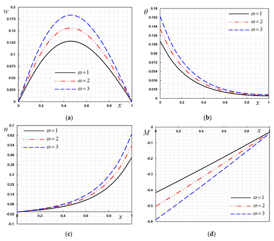
Figure 5. (a) The deflection $\mathrm{w}$ for different thermal vibration frequencies $\mathsf{\omega }$. (b) The temperature $\mathsf{\theta }$ for different thermal vibration frequencies $\mathsf{\omega }$. (c) The displacement $\mathrm{u}$ for different thermal vibration frequencies $\mathsf{\omega }$. (d) The bending moment $M$ for different thermal vibration frequencies $\mathsf{\omega }$.

7. Conclusions

In the current investigation, the thermoelastic vibration of nanobeams under the effect of a harmonic external force and rectified sine wave heating is discussed. Using the nonlocal elasticity theory and non-Fourier heat conduction model, basic equations are derived. The effect of different parameters, such as the nonlocal parameter $\overline{\mathsf{\xi }}$, the magnitude of forcing excitation ${\mathrm{F}}_0$, the angular frequency of thermal vibration $\mathsf{\omega }$ and the frequency of the external excitation $\mathsf{\Omega }$ on the studied fields of the nanobeam was additionally examined. From the obtained results, we found that:

-

The magnitude of forcing excitation, the nonlocal parameter, the frequency of the external excitation and the frequency of the rectified sine wave heating field have a considerable influence on the response of the system behavior.

-

When an external harmonic excitation is applied to the nanobeam, the field quantities are more sensitive to excitation frequencies.

-

The increase in the value of the forcing excitation causes an increase in the thermodynamic temperature values, displacement and in the lateral fields, which is evident in the peak points of the profiles.

-

The results in this study may find applications and requests in the development and design of resonators due to thermal environmental loading.

-

The vibration of the heat response of nanobeams can vary by changing the size of the external force and thermal loads without having to change any other engineering and physical parameters of the nanobeams.

-

The temperature dependence of the frequency of the resonance of resonator devices can be utilized to design and create precision thermometers that are not at all suitable under high sensitivity to rectified sine wave heating and harmonic loads.

References

- Mohammedi, S.; Hassanirad, A. Applied and Theoretical Cantilever Beam Free Vibration Analysis. World Acad. Sci. Eng. Tech. 2012, 61, 1619–1622. [Google Scholar]
- Younis, M.I. MEMS Linear and Non-Linear Statics and Dynamics; Springer: New York, NY, USA, 2011. [Google Scholar]
- Allameh, S.M. An introduction to mechanical-properties-related issues in MEMS structures. J. Mater. Sci. 2003, 38, 4115–4123. [Google Scholar] [CrossRef]
- Abouelregal, A.E. Response of thermoelastic microbeams to a periodic external transverse excitation based on MCS theory. Microsyst. Technol. 2018, 24, 1925–1933. [Google Scholar] [CrossRef]
- Anh, N.D.; Hai, N.Q.; Hieu, D.V. The equivalent linearization method with a weighted averaging for analyzing of nonlinear vibrating systems. Lat. Am. J. Solids Struct. 2017, 14, 1723–1740. [Google Scholar] [CrossRef]
- Sidhardh, S.; Ray, M.C. Size-Dependent elastic response in functionally graded microbeams considering generalized first strain gradient elasticity. Q. J. Mech. Appl. Math 2019, 72, 273–304. [Google Scholar] [CrossRef]
- Abouelregal, A.E.; Zenkour, A.M. Thermoviscoelastic response of an axially loaded beam under laser excitation and resting on Winkler’s foundation. Multidiscip. Model. Mater. Struct. 2019, 15, 1238–1254. [Google Scholar] [CrossRef]
- Gholipour, A.; Ghayesh, M.H.; Zhang, Y. A comparison between elastic and viscoelastic asymmetric dynamics of elastically supported AFG beams. Vibration 2020, 3, 3–17. [Google Scholar] [CrossRef]
- Abouelregal, A.E.; Zenkour, A.M. Thermoelastic problem of an axially moving microbeam subjected to an external transverse excitation. J. Theor. Appl. Mech. 2015, 53, 167–178. [Google Scholar] [CrossRef]
- Farokhi, H.; Ghayesh, M.H.; Gholipour, A. Dynamics of functionally graded micro-cantilevers. Int. J. Eng. Sci. 2017, 115, 117–130. [Google Scholar] [CrossRef]
- Ghayesh, M.H. Mechanics of viscoelastic functionally graded microcantilevers. Eur. J. Mech. A Solids 2019, 73, 492–499. [Google Scholar] [CrossRef]
- Rezazadeh, G.; Khatami, F.; Tahmasebi, A. Investigation of the torsion and bending effects on static stability of electrostatic torsional micro-mirrors. Microsyst. Technol. 2007, 13, 715–722. [Google Scholar] [CrossRef]
- Chen, J.Y.; Hsu, Y.C.; Lee, S.S.; Mukherjee, T.; Fedder, G.K. Modeling and simulation of a condenser microphone. Sens. Actuators A Phys. 2008, 145, 224–230. [Google Scholar] [CrossRef]
- Eringen, A.C. Nonlocal Continuum Field Theories; Springer Verlag: New York, NY, USA, 2002. [Google Scholar]
- Eringen, A.C. On differential equations of nonlocal elasticity and solutions of screw dislocation and surface waves. J. Appl. Phys. 1983, 54, 4703–4710. [Google Scholar] [CrossRef]
- Marin, M.; Craciun, E.M.; Pop, N. Considerations on mixed initial-boundary value problems for micropolar porous bodies. Dyn. Syst. Appl. 2016, 25, 175–196. [Google Scholar]
- Riaz, A.; Ellahi, R.; Bhatti, M.M.; Marin, M. Study of heat and mass transfer in the Eyring—Powell model of fluid propagating peristaltically through a rectangular compliant channel. Heat. Transf. Res. 2019, 50, 1539–1560. [Google Scholar] [CrossRef]
- Bhatti, M.M.; Ellahi, R.; Zeeshan, A.; Marin, M.; Ijaz, N. Numerical study of heat transfer and Hall current impact on peristaltic propulsion of particle-fluid suspension with compliant wall properties. Mod. Phys. Lett. B 2019, 33, 1950439. [Google Scholar] [CrossRef]
- Warminska, A.; Manoach, E.; Warminski, J. Vibrations of a composite beam under thermal and mechanical loadings. Procedia Eng. 2016, 144, 959–966. [Google Scholar] [CrossRef][Green Version]
- Warminska, A.; Warminski, J.; Manoach, E. Nonlinear dynamics of a reduced multimodal Timoshenko beam subjected to thermal and mechanical loadings. Meccanica 2014, 49, 1775–1793. [Google Scholar] [CrossRef]
- Alcheikh, N.; Tella, S.A.; Younis, M.I. Adjustable static and dynamic actuation of clamped-guided beams using electrothermal axial loads. Sens. Actuators A Phys. 2018, 273, 19–29. [Google Scholar] [CrossRef]
- Chang, T.; Fu, Y.M.; Dai, H.L. Nonlinear dynamic analysis of fiber metal laminated beams subjected to moving loads in thermal environment. Compos. Struct. 2016, 140, 410–416. [Google Scholar]
- Abouelregal, A.E.; Zenkour, A.M. Thermoelastic response of nanobeam resonators subjected to exponential decaying time varying load. J. Theor. Appl. Mech. 2017, 55, 937–948. [Google Scholar] [CrossRef][Green Version]
- Zenkour, A.M.; Abouelregal, A.E. Decaying temperature and dynamic response of a thermoelastic nanobeam to a moving load. Adv. Comput. Des. 2018, 3, 1–16. [Google Scholar]
- Lord, H.W.; Shulman, Y. A generalized dynamical theory of thermoelasticity. J. Mech. Phys. Solids 1967, 15, 299–309. [Google Scholar] [CrossRef]
- Hanig, G.; Hirdes, U. A method for the numerical inversion of Laplace transform. J. Comput. Appl. Math 1984, 10, 113–132. [Google Scholar] [CrossRef]
- Zhang, Y.Q.; Liu, G.R.; Xie, X.Y. Free transverse vibrations of double-walled carbon nanotubes using a theory of nonlocal elasticity. Phys. Rev. B 2005, 71, 195–404. [Google Scholar] [CrossRef]
- Tzou, D.Y. Macro-To Microscale Heat Transfer: The Lagging Behavior; John Wiley & Sons: Hoboken, NJ, USA, 2014. [Google Scholar]
- Harrington, D.A.; Mohanty, P.; Roukes, M.L. Energy dissipation in suspended micromechanical resonators at low temperatures. Phys. B Condens. Matter 2000, 284, 2145–2146. [Google Scholar] [CrossRef]
© 2020 by the authors. Licensee MDPI, Basel, Switzerland. This article is an open access article distributed under the terms and conditions of the Creative Commons Attribution (CC BY) license (http://creativecommons.org/licenses/by/4.0/).