Article

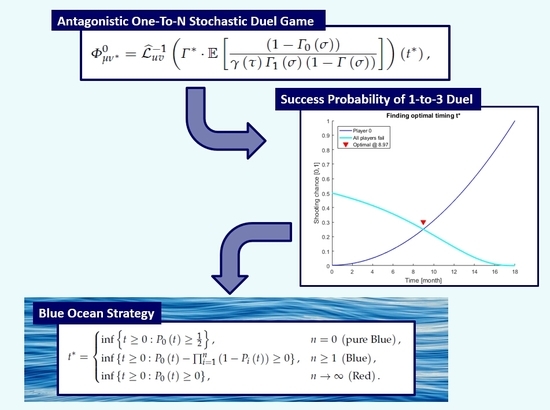
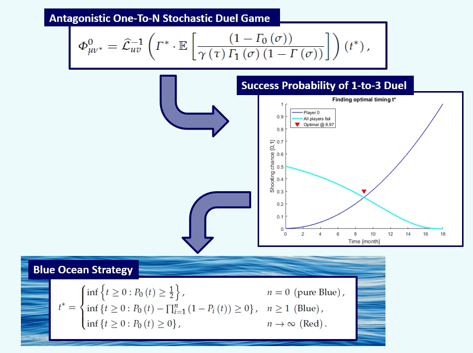
Antagonistic One-To-N Stochastic Duel Game

by
Song-Kyoo (Amang) Kim
School of Applied Sciences, Macao Polytechnic Institute, Macao
R. de Luis Gonzaga Gomes, Macao.
Mathematics 2020, 8(7), 1114; https://doi.org/10.3390/math8071114
Submission received: 10 June 2020 / Revised: 2 July 2020 / Accepted: 2 July 2020 / Published: 6 July 2020
(This article belongs to the Special Issue Queue and Stochastic Models for Operations Research)

Abstract

:
This paper is dealing with a multiple person game model under the antagonistic duel type setup. The unique multiple person duel game with the one-shooting-to-kill-all condition is analytically solved and the explicit formulas are obtained to determine the time dependent duel game model by using the first exceed theory. The model could be directly applied into real-world situations and an analogue of the theory in the paper is designed for solving the best shooting time for hitting all other players at once which optimizes the payoff function under random time conditions. It also mathematically explains to build the marketing strategies for the entry timing for both blue and red ocean markets.

Graphical Abstract

1. Introduction

A hybrid stochastic game model becomes more flexible to solve various duel type game problems more effectively [1,2,3]. In the versatile two-person stochastic duel game [4], the joint functional of the standard stopping game has been constructed to analyze the decision-making parameters in the time domain. An extended version of a versatile stochastic duel game for multiple players is designed as a successor of the recent research by the author [4]. The antagonistic 1-to-n stochastic duel game is an n + 1 person duel type game of which each player could choose either to “shoot” to kill all other players at once or “wait” for one step closer to the target on his turn (or iteration) but, unlike a conventional two person duel game, a player is shooting the rest of players at once (i.e., one-shooting-to-kill-all) when the player decides to take a shoot. It is more like players to use an automatic machine gun instead of a single bullet gun but each player can take a shoot only once on his turn.
The topic regarding market entry strategies has been massively studied [5,6,7,8,9,10] and many studies bring different ideas and terminologies including first-movers, fast-followers [11,12,13,14], and late-movers [15,16,17]. The terminologies of the red ocean (market) and the blue ocean (market) have been represented by the book titled “Blue Ocean Strategy” [18]. The red ocean represents all markets in existence today. In the red ocean, industry boundaries are already defined and accepted, and the competitive rules of the game are well-known. Contrarily, the blue ocean strategy is about creating and capturing uncontested market space and the simultaneous pursuit of differentiation to open up a new market space [18]. The blue ocean strategy [18] finds the value that crosses conventional market segmentation and offering value and lower cost. It is about creating and capturing uncontested market space, thereby making the competition irrelevant [19]. The number of competitors in a market is a typical factor for determining either the blue or red oceans. The market which has a relatively small number of competitors is still considered as a blue ocean market and, as you could guess, the red ocean market has a relatively large number of competitors who are involved in the market. Many studies have been done for delivering the best strategies for the first shooting based on game theories [4,20,21,22,23,24] and a conventional way to categorize the market condition is dividing into the blue and the red oceans [18,19]. The mathematical implications for finding the best entrant strategies based on various market status is demonstrated in the further section. Additionally, this paper also demonstrates the special case of a 1-to-n stochastic duel game to adapt the memoryless iteration processes for all players. This special case shows how the 1-to-n stochastic duel game could be applied into the memoryless condition including development cycles of IT products without impacts from past information.
The paper is organized as follows: Section 2 provides the model that finds the moment where the decision making occurs based on a marked point process in time domains. This section also contains empirical studies to show how this new model is working properly. The blue and red ocean strategies are fully described in Section 3 by the proposed mathematical implications and this new antagonistic multiple-player duel game with memoryless conditions has been applied in a high-tech product market in Section 4. Finally, the conclusion is included in Section 5.

2. Antagonistic One-To-N Duel Game

The antagonistic stochastic duel game of n + 1 players (called “A” and the rest of player Bs “ 1 , , n ”) are introduced and all players know the full information regarding the success probabilities based on the time domain. Each player has two strategies either “shoot” or “wait”, and choose one strategy after completing each iteration. Unlike a conventional two person duel game, it has the one-shooting-to-kill-all condition which means each player has n bullets that can be applied at once to kill the rest of players. That is the reason why it is called as a 1-to-n person duel game rather than called as an n + 1 person duel game.

Preliminaries

Let us consider the 1-to-n person antagonistic duel game with the pure strategy. Each player has two strategies either “shoot (to kill all at once)” or wait and choose one strategy at the certain points of time. Let A s be a payoff (related) function of player A based on the continues time s and B i t , i = 1 , , n be payoff (related) functions of players B i at the time t. The payoff functions of all players are assigned as follows:
{ A ( s ) : 0 A ( s ) A ( s + Δ ) , s [ 0 , s max ) , s max R + , Δ > 0 } ,
{ B i ( t ) : 0 B i ( t ) B i ( t + Δ ) , t [ 0 , t i max ) , t i max R + , Δ > 0 , i = 1 , , n }
and all these functions are monotone nondecreasing which are common in duel type games [21,25,26]. The accumulative success probability functions of players [4] could be assigned as follows:
P 0 s : = A s A s max , P i t : = B i t B t i max , i = 1 , , n .
The best strategy for each player in a 1-to-n duel game is the moment to hit others at once. As it is shown in Figure 1, the accumulative success probabilities of all players are arbitrary incremental continuous functions which reaches 1 when the time s (or t) meets the allowed maximum s max , t i max < .
In duel games, a certain point t * maximizes the chance for succeeding the shoot [25,26,27] and this best point is the moment of the success in the continuous time domain:
t * = inf t 0 : P 0 t i = 1 n 1 P i t 0 .
It is noted that each player can make the decision at certain points of time and that is the reason why it becomes a discrete time series although the success probabilities are continuous functions.
In the case of the 4 person duel game in Figure 1, the best shooting time for player A (or player 0) is 8.97 months with the 25.06 percents winning chance of the game (see Figure 2). Let ( Ω , F ( Ω ), P) be a probability time space and let F S , F T i F Ω be independent σ -subalgebras. Suppose
S : = j 0 ε S j , 0 = S 0 < S 1 < , a . s .
T i : = k 0 ε T k i , 0 = T 0 i < T 1 i < , i = 1 , , n , a . s .
are F S -measurable and F T i -measurable renewal point processes ( ε a is a point mass at a) which are associated with the moments of executing the strategies of players. These processes are with the following notation for player A:
σ : = σ j = S j S j 1 , j = 1 , 2 , , 0 , j 0 ,
and other player Bs, 1 , , n ,
τ i : = τ k i = T k i T k 1 i , k = 1 , 2 , , 0 , k 0 .
We can evaluate the functional
δ 0 θ = E e θ σ , δ i θ = E e θ τ i , Re θ 0 ,
and
δ θ = E e θ τ , τ = 1 n i = 1 n τ i .
The game in the paper is a stochastic process describing the evolution of conflicting between players with the completed information [28] which indicates that the success probabilities of players are known [4]. Only on the j-th epoch S j , player A could make the decision either for taking a shoot or for waiting until another turn (iteration) S j + 1 . Player A could beat all other players by exceeding their respective threshold M (or N i for other players i 1 , 2 , , n ). To further formalize the game, the exit indices are introduced as follows:
μ : = inf j : S j = S 0 = 0 + σ 1 + + σ j M ,
ν i : = inf k : T k i = T 0 i = 0 + τ 1 + + τ k i N i , i = 1 , , n .
In the time domain of duel games, the threshold of each player could be converged into one value t * from (4). Due to the backward induction, player A will have the best chance to succeed for shooting compare to the failure chance of other players ( P 0 S μ and i = 1 n 1 P i T ν i i , respectively). Hence, player A has the highest success probability of shooting at time S μ , unless at least one of the other players does not reach his best shooting chance at time T ν i . Thus, the game is ended at min S μ , T ν 1 1 , T ν 2 2 , T ν n n . However, we are targeting the confined duel game for player A on trace σ -algebra F Ω P 0 t i = 1 n 1 P i t 0 S μ T ν * : = min T ν 1 1 , T ν 2 2 , T ν n n (i.e., player A hits first). The functional
Φ μ ν * 0 = Φ μ ν * 0 θ 0 , θ 1 = E e θ 0 S μ 1 θ 1 S μ · 1 S μ T ν * 1 P 0 t i = 1 n 1 P i t ,
Re θ 0 0 , Re θ 1 0 ,
where
ν * : = ν k : min T ν 1 1 , T ν 2 2 , , T ν n n ,
of the game will represent the status of player A (also called player 0) and the rest of players upon the exit time S μ and the pre-exit time S μ 1 [1,2,3]. The Laplace–Carson transform is applied as follows:
L ^ p q u , v = u v p = 0 p = 0 e u p v q d p , q , Re u > 0 , Re v > 0 ,
with the inverse
L ^ u v 1 p , q = L 1 1 u v ,
and
L ^ u v 1 r = L ^ u v 1 p , q | p , q r , r
where L 1 is the inverse of the bivariate Laplace transform [29].
Theorem 1.
The functional Φ μ ν 0 for player A in the game on trace σ-algebra F Ω P 0 S μ + i = 1 n 1 P i T ν i 0 S μ T ν * satisfies the following formula:
Φ μ ν * 0 = L ^ u v 1 Γ * · E 1 Γ 0 σ γ τ Γ 1 σ 1 Γ σ t * ,
where
γ ( x , t ) = e x t ,
γ ( t ) : = γ ( v , t ) ,
Γ 0 ( t ) : = γ ( u , t ) ,
Γ 1 ( t ) : = γ ( θ 0 + u , t ) ,
Γ 2 ( t ) : = γ ( θ 0 + θ 1 + u , t ) ,
Γ ( t ) : = γ ( t ) · Γ 2 ( t ) ,
Γ * : = γ ( t * ) · Γ 2 ( t * ) .
Proof. 
To establish an explicit formula for Φ μ ν 0 , we introduce the following families:
μ p = inf m : S m > p ,
ν * q = k l : min T k 1 1 , T k 2 2 , , T k n n > q ,
T k = T k i : min T k 1 , T k 2 , , T k n > q .
Application for L ^ p q to Φ μ p ν * q will bypass all terms except for S μ < T ν P 0 t i = 1 n 1 P i t 0 . Thus, applying operator L ^ p q to random set 1 μ p = j , ν * q = k : p 0 , q 0 , we arrive at
L ^ p q 1 μ p = j , ν * q = k u , v = e u S j 1 e u S j e v T k 1 * e v T k * .
To prove formula (30), we first notice that
1 μ p = j , ν * q = k = 1 S j 1 p 1 S j > p 1 T k 1 * q 1 T k * > q .
Then, iterating the integral of (16),
L ^ p q 1 μ p = j , ν q = k u , v = p = S j 1 S j e u p d p q = T k 1 T k e v q d q
which yields (30). Denote
Ψ u , v : = L ^ p q Φ μ p ν * q u , v
Since,
Φ μ p ν q 0 = j 0 E [ k 0 E [ e θ 0 S j 1 θ 1 S j    · e ϑ 0 T k 1 ϑ 1 T k × 1 μ p = j , ν * q = k · 1 S μ t 0 , T ν * > S μ ]
where
1 S μ < T ν * · 1 P S μ i 1 , , n 1 P i T ν i = 1 t * S μ < T ν * ,
then by Fubini’s Theorem and due to (30) and (33),
Ψ u , v = j 0 E [ k > t * / τ E [ e θ 0 S j 1 θ 1 S j    · e ϑ 0 T k 1 ϑ 1 T k e u S j 1 e u S j e v T k 1 * e v T k * × 1 t * S μ < T ν * ] = E j 0 R 1 j k > σ τ j R 2 j k
where
R 1 j = e θ 0 + u j 1 σ θ 1 σ j 1 e u σ × 1 P S μ i 1 , , n 1 P i T ν i = e θ 0 + u σ 1 Γ 0 σ Γ 2 σ j × 1 S k t * , R 2 k = e ϑ 0 + v τ k 1 ϑ 1 τ k 1 e v τ ,
and
k > σ τ j R 2 j k = k > σ τ j e v τ 1 e v τ e v τ k     = e v τ 1 e v τ · k > σ τ j e v τ k = 1 γ τ γ σ j .
Then, we have
Ψ u , v = E 1 Γ 0 σ γ τ Γ 1 σ j t * σ Γ σ j = Γ * · E 1 Γ 0 σ γ 1 τ Γ 1 σ 1 Γ σ .
Now, Φ μ p ν * q 0 can be revived when the inverse of the operator L ^ p q of (17) to Ψ u , v :
Φ μ ν * 0 = L ^ u v 1 Γ * · E 1 Γ 0 σ γ τ Γ 1 σ 1 Γ σ t * .
The functional Φ μ ν 0 has all of the decision making parameters of player A. The information includes the best shooting moments ( S μ ; exit time), the one step prior to each best shooting moment ( S μ 1 ; pre-exit time), and the optimal number of iterations for player A. The information from the closed functional is as follows:
E [ e θ S μ ] = Φ μ ν * 0 ( 0 , θ ) ,
E [ S μ ] = lim θ 0 ( θ ) Φ μ ν * 0 ( 0 , θ ) ,
E [ S μ 1 ] = lim θ 0 ( θ ) Φ μ ν * 0 ( θ , 0 ) .

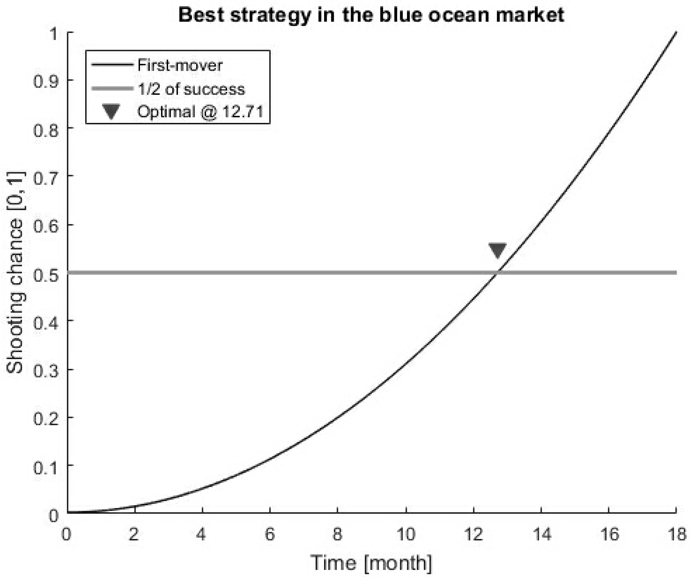
3. Best Strategies in Blue and Red Ocean Markets

Companies in the red ocean markets try to beat their competitors for a greater share of product or service demand. As the market space gets competitive, profits and growth are reduced [18,19]. Hence, the strategies of the red ocean are traditional competition-based strategies and practitioners of the red ocean strategy focus on building advantages over competitions by assessing what competitors do and striving to do it better. In the blue ocean market, competition is irrelevant because demand is created rather than competed by rivals. It is noted that deeper potential of market space that is not yet explored [18,19]. In general, markets are evolving from the blue ocean to the red ocean. All red ocean markets are started from the blue ocean and all successful blue ocean markets eventually will become the red oceans because all companies will try to enter successful markets. The timing of entering markets is vital to build a new business successfully regardless which oceans are targeted [5,6]. Many companies might overestimate market potentials of the blue ocean and underestimated the time and effort needed to create a real market presence. Entrants might be able to recoup their investment to boost the new market. In this case, fast-followers can benefit funded by the first-movers and leapfrog into earlier profitability [7]. The related strategies and terminologies including first-movers, fast-followers [11,12,13,14], and late-movers [15,16,17] are widely studied. Unfortunately, many studies are controversial and these studies have argued which strategies are better than others and try to deliver the critical factors and the market conditions to be succeed when companies chose a certain strategy [11,12,13,14,15,16,17]. The pure blue ocean market could be counted if none of other companies are involved except for the one who creates the market.
The 1-to-n stochastic duel game in this paper could be adapted to find the moment of the new entrants either in the blue or the red oceans based on the number of competitors. From (4), the moment of the success t * is changed based on the market conditions. In atypical blue ocean market, the moment t * shall be the same as a conventional 1-to-n duel game which has been introduced in the previous section from (4), but it shall be different when the market becomes the red ocean:
t * = inf t 0 : P 0 t 0
because i = 1 n 1 P i t 0 when n . It means that a new entrant should launch their products as soon as possible. Due to the backward induction, sooner launching gives the better chance to succeed in the red ocean market regardless of the success probability that a new entrant has. In general, the blue ocean does not distinguish between only one company and a small number of companies in a new market but the number of the competitors in the blue ocean market actually determines the strategy whether a new entrant becomes a first-mover or a fast-follower. Theoretically speaking, the market which has more than one company is not the blue ocean market although this market is considered as the blue ocean in practice. The pure blue ocean market is a totally new market and there is no one else except for one who actually creates the market. This becomes another special case for finding the success moment from (4):
t * = inf t 0 : P 0 t 1 2 , n = 0 ,
and it indicates that the first-mover strategy is not applicable in the pure blue ocean markets. Unlike the red ocean markets, the new entrants in the totally new market should wait until they have more than 50 percent chance to win the game (see Figure 3). It is noted that the market status is dramatically changed as soon as other firms are involved in this market (i.e., n 1 ). From (4), (40) and (41), the moment of success before finding the best strategies could be summarized as follows:
t * = inf t 0 : P 0 t 1 2 , n = 0 pure Blue , inf t 0 : P 0 t i = 1 n 1 P i t 0 , n 1 Blue , inf t 0 : P 0 t 0 , n Red .
Finding the best strategies for entering the market is straight forward after determining the moment of success t * based on the market status by using the functional from (4).

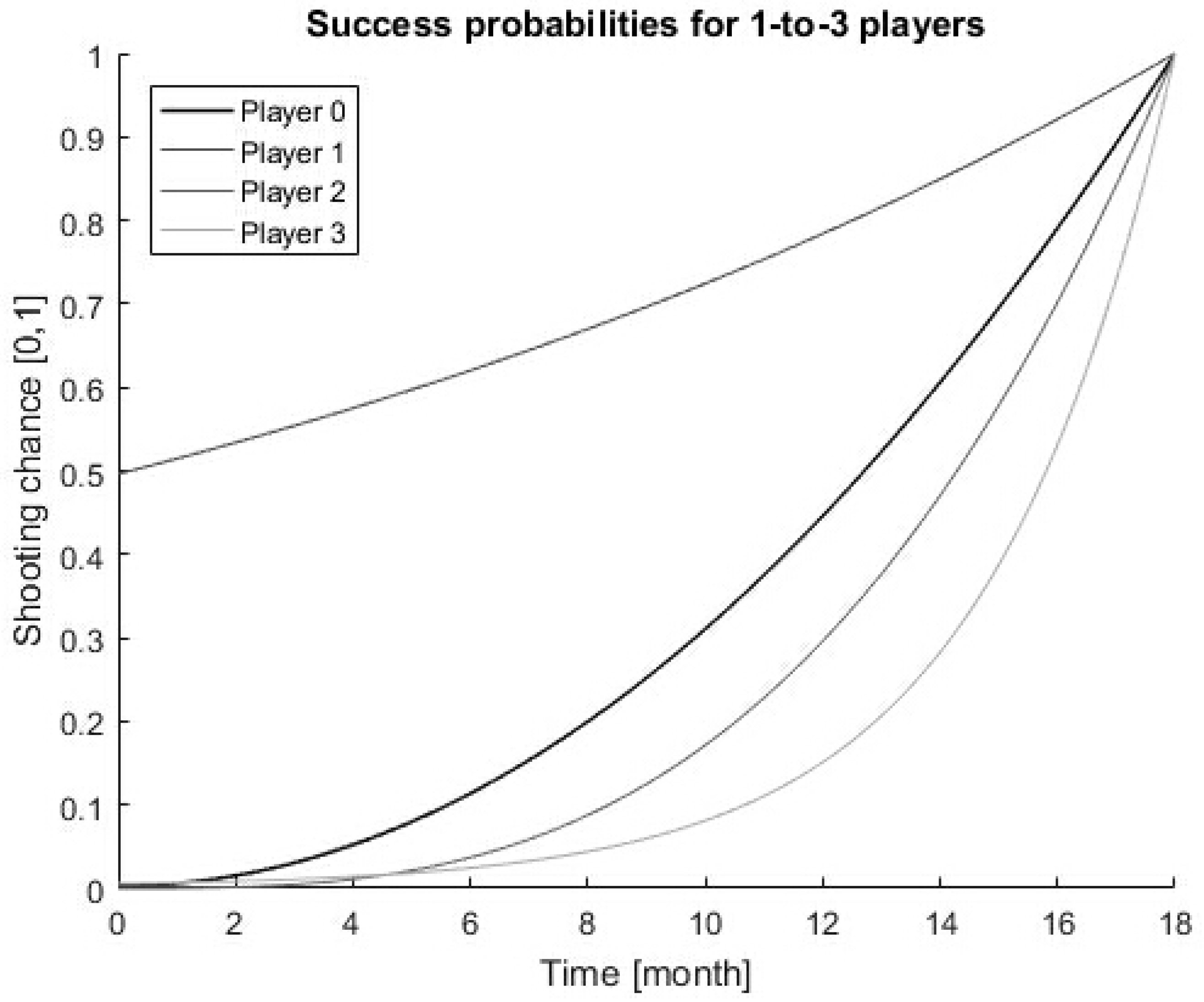
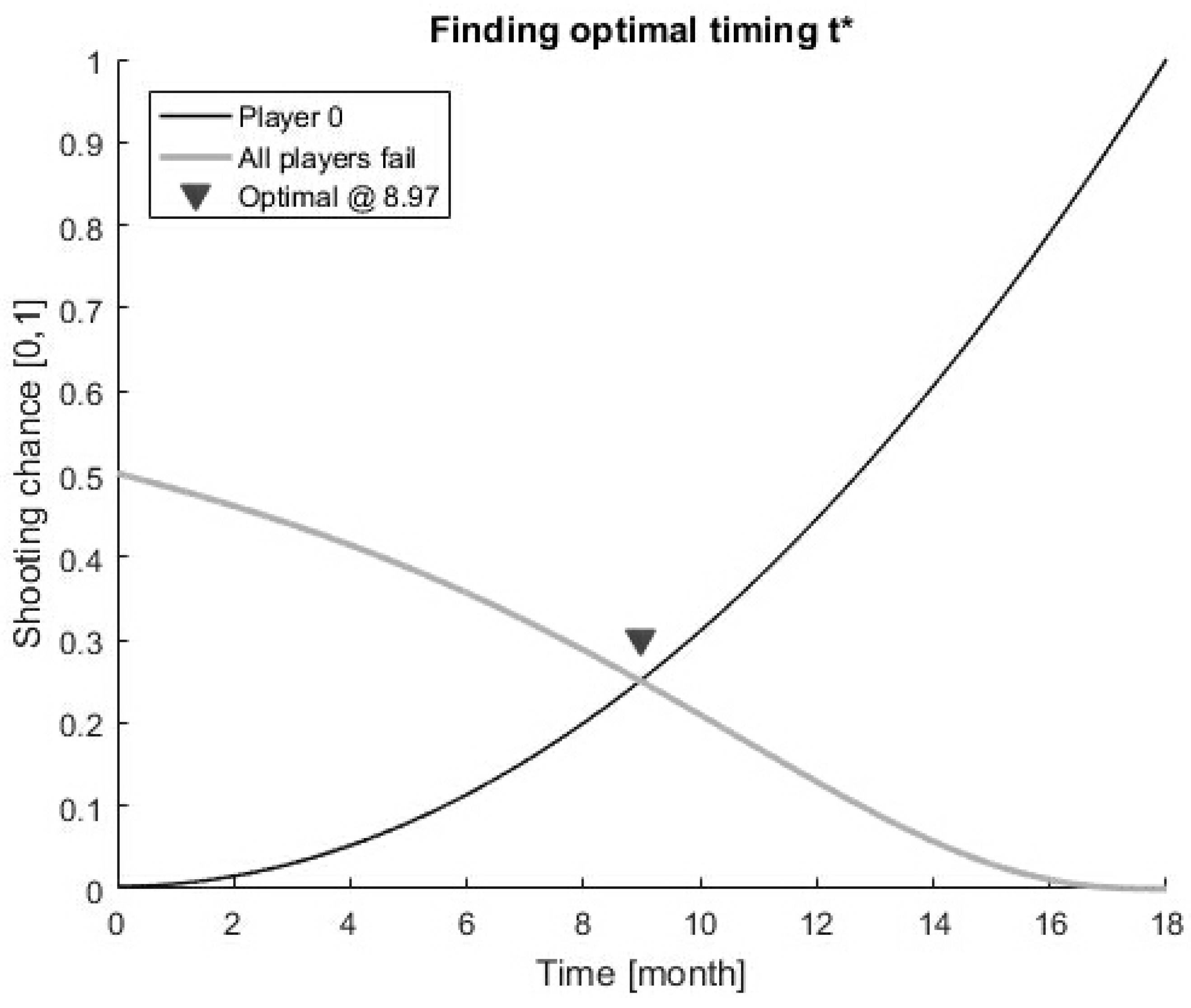
4. Memoryless Case: IT Product Launch Strategy for Multiple Competitors

This section deals with the memoryless property for the iteration time of each player. It means that the past iteration processes do not impact on the present iteration process and each iteration duration is exponentially distributed. This type of iteration process could present the development cycle of IT products including smartphones and PCs. Once an IT product is ready, the history of past development cycles shall not be what really matters. Therefore, this first case is easily adapted into the decision making for new IT product development. The second case deals with the marketing strategies based on the market conditions. A typical way to categorize markets would the blue and the red oceans [18] and there are massive studies regarding the timing of entering markets for new entrants [5,6,7,8,9,10]. All studies have agreed that the strategies for the new entrants depend on the market status although they have still argued which strategy is better than others [11,12,13,14,15,16,17]. This case will give some ideas on when to enter the markets based on the mathematical implications.
This section shows the case of the memoryless iteration time for player A verses other players in a stochastic duel game. Each iteration duration is exponentially distributed for player A and others with:
E σ = 1 λ a , E τ = 1 λ ,
from (8) and (9). The continuous time domain duel game could be flexible by using any incremental continuous cost functions. It is assumed that the best moment in a duel game is already known as t * from (1)–(4). As a result that the memoryless iteration process of each player is considered, the duration of one iteration for each player is exponentially distributed. From (10), we have:
E e u σ = λ a λ a + u , E e v τ = λ λ + v .
Lemma 1.
The functional Φ μ ν * 0 to find E e θ 1 S μ based on the memoryless iteration durations (37) is as follows:
Φ μ ν * 0 0 , θ 1 = 1 + λ a e t * θ 1 .
Proof. 
As a result of the memoryless properties, let us consider that each iteration process is exponentially distributed with both the duration of the iteration 1 / λ a for player A and 1 / λ for the rest of players. We are targeting to find E S μ from (17) and (37). The related functionals from (20)–(26) are revised as follows:
Γ 0 t = Γ 1 t : = γ u , t ,
Γ 2 t : = γ θ 1 + u , t ,
and
Φ μ ν * 0 = L ^ u v 1 Γ * · E 1 γ u , σ γ v , τ γ u , σ 1 γ v , σ · γ θ 1 + u , σ t *
where
E 1 γ u , σ γ v , τ γ u , σ 1 γ v , σ · γ θ 1 + u , σ = E 1 γ u , σ γ u , σ 1 γ v , σ · γ θ 1 + u , σ E 1 γ v , τ ,
E 1 γ v , τ = E e v τ = λ λ v , E 1 γ u , σ · Γ * γ u , σ 1 γ v , σ · γ θ 1 + u , σ = E 1 e u σ e v t * · e u t * · e θ 1 t * 1 e u σ + e θ 1 + v σ 1 e u + θ 1 + v σ = E e u + v + θ 1 t * e u σ + E e u + v + θ 1 t * e θ 1 + v σ 1 e u + θ 1 + v σ     E e u σ e u + v + θ 1 t * e u σ E e u σ e u + v + θ 1 t * e θ 1 + v σ 1 e u + θ 1 + v σ
= R 1 + R 2 R 3 R 4 .
To get R 1 , R 2 , R 3 , and R 4 ,
R 1 = E [ e ( u + v + θ 1 ) t * e u σ ] = e ( u + v + θ 1 ) t * E [ e u σ ] = e ( u + v + θ 1 ) t * { λ a λ a u } ,
R 2 = E [ e ( u + v + θ 1 ) t * ( e ( θ 1 + v ) σ ) ( 1 e ( u + θ 1 + v ) σ ) ] = e ( u + v + θ 1 ) t * · k = 0 λ a λ a + ( k + 1 ) ( θ 1 + v ) + k u ,
R 3 = E [ e u σ e ( u + v + θ 1 ) t * e u σ ] = e ( u + v + θ 1 ) t * ,
R 4 = E [ e u σ e ( u + v + θ 1 ) t * ( e ( θ 1 + v ) σ ) ( 1 e ( u + θ 1 + v ) σ ) ] = e ( u + v + θ 1 ) t * · k = 1 λ a λ a + k ( u + θ 1 + v ) .
From (52)–(55), we have:
R 1 = e u + v + θ 1 t * λ a λ a u , R 2 = e u + v + θ 1 t * · k = 0 λ a λ a + k u + k + 1 θ 1 + v , R 3 = e u + v + θ 1 t * , R 4 = e u + v + θ 1 t * · k = 1 λ a λ a + k u + θ 1 + v ,
and, from (18),
Φ μ ν * 0 ( 0 , θ 1 ) = L ^ u v 1 [ R 1 + R 2 R 3 R 4 ] [ λ λ v ] | ( r = t * )
= L ^ u v 1 [ λ λ v ] [ λ a e ( u + v + θ 1 ) t * λ a u ] + L ^ u v 1 [ λ λ v ] [ k = 0 λ a e ( u + v + θ 1 ) t * λ a + ( θ 1 + v ) + k ( u + θ 1 + v ) ] L ^ u v 1 [ λ λ v ] [ e ( u + v + θ 1 ) t * ] L ^ u v 1 [ λ λ v ] [ k = 1 λ a e ( u + v + θ 1 ) t * λ a + k ( u + θ 1 + v ) ] = [ J 1 + J 2 J 3 J 4 ] | ( r = t * ) ,
where
J 1 = L ^ u v 1 [ λ a e ( u + v + θ 1 ) t * λ a u ] = e t * θ 1 ( e λ a ( t t * ) 1 ) ( e λ b ( t t * ) 1 ) 1 t t * ,
J 2 = L ^ u v 1 [ λ λ v ] [ k = 0 λ a e ( u + v + θ 1 ) t * λ a + ( k + 1 ) ( θ 1 + v ) + k u ] = 0 ,
J 3 = L ^ u v 1 [ λ λ v ] [ λ a e ( u + v + θ 1 ) t * ] = ( λ a e t * θ 1 ) e λ ( t t * ) 1 1 t t * ,
J 4 = L ^ u v 1 [ λ λ v ] [ k = 1 λ a e ( u + v + θ 1 ) t * λ a + k ( u + θ 1 + v ) ] = 0 .
From (18) and (57)–(61), we have
Φ μ ν * 0 ( 0 , θ 1 ) = [ J 1 J 3 ] | ( r = t * ) = e t * θ 1 ( 1 λ a ) ( 1 ) ,
and, from (62),
E e θ 1 S μ = 1 + λ a e t * θ 1 .
From (45), (38) yields
E S μ = lim θ 1 0 θ 1 Φ μ ν * 0 0 , θ 1 = t * 1 + λ a .
The best response is the strategy which produce the most favorable outcome for a player [3]. The best response of player A is the exit index of shooting μ and it responds based on the iteration time of other players and the function of the best response of player A is as follows:
E μ ν * = λ a t * 1 + λ a .
As a result of the backward induction, the best response of player A is not related with the iteration cycles of other players.

5. Conclusions

The new type of an antagonistic n + 1 person stochastic duel game has been studied. In this versatile stochastic duel game, players could have random iterations in the time domain under the one-shooting-to-kill-all condition which allows that each player has exact n bullets for shooting at once to kill the rest of players. A joint functional of the process has been constructed to analyze the information of decision making parameters which gives the best chance of the player to win the time domain game. The compact closed forms have been obtained and the analytical approach is fully supported to understand the core of the 1-to-n stochastic duel game by applying into a strategic problem in the blue ocean market cases. Furthermore, the guideline for the mathematical implications for adapting this 1-to-n duel game in a realistic situation has also been invested in details for future studies.

Funding

This research received no external funding.

Acknowledgments

Special thanks to the Guest Editor, Tuan Phung-Duc, who guides the author to submit the proper topic of the journal and also thankful to the referees whose comments are very constructive. There are no available data to be stated.

Conflicts of Interest

The author declares no conflict of interest.

References

  1. Dshalalow, J.H.; White, R. On Reliability of Stochastic Networks. Neural Parallel Sci. Comput. 2013, 21, 141–160. [Google Scholar]
  2. Dshalalow, J.H.; Iwezulu, K.; White, R.T. Discrete Operational Calculus in Delayed Stochastic Games. Neural Parallel Sci. Comput. 2016, 24, 55–64. [Google Scholar]
  3. Kim, S.-K. Blockchain Governance Game. Comp. Indust. Eng. 2019, 136, 373–380. [Google Scholar] [CrossRef] [Green Version]
  4. Kim, S.-K. A Versatile Stochastic Duel Game. Mathematics 2020, 8, 678. [Google Scholar] [CrossRef]
  5. Thomas, R.J. Timing—The Key to Market Entry. J. Consum. Mark. 1985, 2, 77–87. [Google Scholar] [CrossRef]
  6. Saylor Academy, Fundamentals of Global Strategy, 2019. Available online: https://saylordotorg.github.io/text/fundamentals-of-global-strategy/index.html (accessed on 1 May 2019).
  7. GTellis, J.; Golder, P.N.; Christensen, C.M. Will and Vision: How Latecomers Grow to Dominate Markets; McGraw-Hill: Princeton, NJ, USA, 2001. [Google Scholar]
  8. Eliashberg, J.; Jeuland, A.P. The Impact of Competitive Entry in a Developing Market upon Dynamic Pricing Strategies. Mark. Sci. 1986, 5, 20–36. [Google Scholar] [CrossRef]
  9. Kalyanaram, G.; Gurumurthy, R. Market Entry Strategies: Pioneers Versus Late Arrivals. Available online: http://www.strategy-business.com/article/18881?gko=c8128 (accessed on 1 May 2019).
  10. Lilien, G.L.; Yoon, E. The Timing of Competitive Market Entry: An Exploratory Study of New Industrial Products. Manag. Sci. 1990, 36, 519–641. [Google Scholar] [CrossRef] [Green Version]
  11. Singh, D. First Mover Or Fast Follower—Why It is Okay to be Either in Tech. 2018. Available online: https://blog.alore.io/first-movers-vs-fast-followers/ (accessed on 1 May 2019).
  12. Birger, J. Second-Mover Advantage. CNN Money. 2006. Available online: https://money.cnn.com/magazines/fortune/fortune_archive/2006/03/20/8371782/ (accessed on 1 May 2019).
  13. Shevlin, R. The Fast Follower Fallacy. The Financial Brand, 2016. Available online: https://thefinancialbrand.com/59369/fast-follower-fallacy/ (accessed on 1 May 2019).
  14. Anthony, S.D. First Mover or Fast Follower. Harv. Bus. Rev. 2012. Available online: https://hbr.org/2012/06/first-mover-or-fast-follower (accessed on 1 May 2019).
  15. Querbes, A.; Frenken, K. Evolving user needs and late-mover advantage. Strateg. Organ. 2017, 15, 67–90. [Google Scholar] [CrossRef] [PubMed] [Green Version]
  16. Shankar, V.; Carpenter, G.S.; Krishnamurthi, L. Late Mover Advantage: How Innovative Late Entrants Outsell Pioneers. J. Mark. Res. 1998, 35, 54–70. [Google Scholar] [CrossRef]
  17. Wunker, S. Better growth decisions: Early mover, fast follower or late follower? Strategy Leadersh. 2012, 40, 43–48. [Google Scholar] [CrossRef] [Green Version]
  18. Kim, W.C.; Mauborgne, R. Blue Ocean Strategy: How to Create Uncontested Market Space and Make the Competition Irrelevant; Harvard Business School Press: Boston, MA, USA, 2004. [Google Scholar]
  19. Internet Archive, A Conversation with W. Chan Kim and Renee Mauborgne, 2005. Available online: https://web.archive.org/web/20081203070029/http://www.insead.edu/alumni/newsletter/February2005/Interview.pdf (accessed on 1 May 2019).
  20. Radzik, T. Games of Timing Related to Distribution of Resources. J. Optim. Theory Appl. 1988, 58, 443–471. [Google Scholar] [CrossRef]
  21. Radzik, T. Silent Mixed Duels. Optimization 1989, 20, 553–556. [Google Scholar] [CrossRef]
  22. Khalfallah, H.; Rious, V. A game theoretical analysis of the design options of the realtime electricity market. Energy Stud. Rev. 2013, 20, 34–64. [Google Scholar] [CrossRef] [Green Version]
  23. Kuenle, H.-U. Markov Games under a Geometric Drift Condition; Advances in Dynamic Games; Springer: New York, NY, USA, 2005; pp. 21–38. [Google Scholar]
  24. Nikoukhah, R.; Delebecque, F. On a stochastic differential game and its relationship with mixed H/H control. In Proceedings of the American Control Conference, Chicago, IL, USA, 24–26 June 1992; IEEE: Piscataway, NJ, USA, 1992; pp. 1380–1384. [Google Scholar]
  25. Lang, J.P.; Kimeldorf, G. Duels with continuous firing. Manag. Sci. 1975, 22, 470–476. [Google Scholar] [CrossRef]
  26. Polak, B. Discussion of Duel. Open Yale Courses, 2008. Available online: http://oyc.yale.edu/economics/econ-159/lecture-16 (accessed on 1 May 2019).
  27. Lang, J.P.; Kimeldorf, G. Silent Duels with Non Discrete Firing. SIAM J. Appl. Math. 1976, 31, 9–110. [Google Scholar] [CrossRef]
  28. Schwalbe, U.; Walker, P. Zermelo and the Early History of Game Theory. Games Econ. Behav. 2001, 34, 123–137. [Google Scholar] [CrossRef] [Green Version]
  29. Dshalalow, J.H.; Ke, H.-J. Layers of noncooperative games. Nonlinear Anal. 2009, 71, 283–291. [Google Scholar] [CrossRef]
Figure 1. Success probabilities for 1-to-3 duel games (4-person game).
Mathematics 08 01114 g001
Figure 2. Best shooting moment t * .
Mathematics 08 01114 g002
Figure 3. Best strategy for a first-mover in the pure blue ocean market.
Mathematics 08 01114 g003

