Study of Local Convergence and Dynamics of a King-Like Two-Step Method with Applications

 ,
,  ,
,  ,
,  and
and 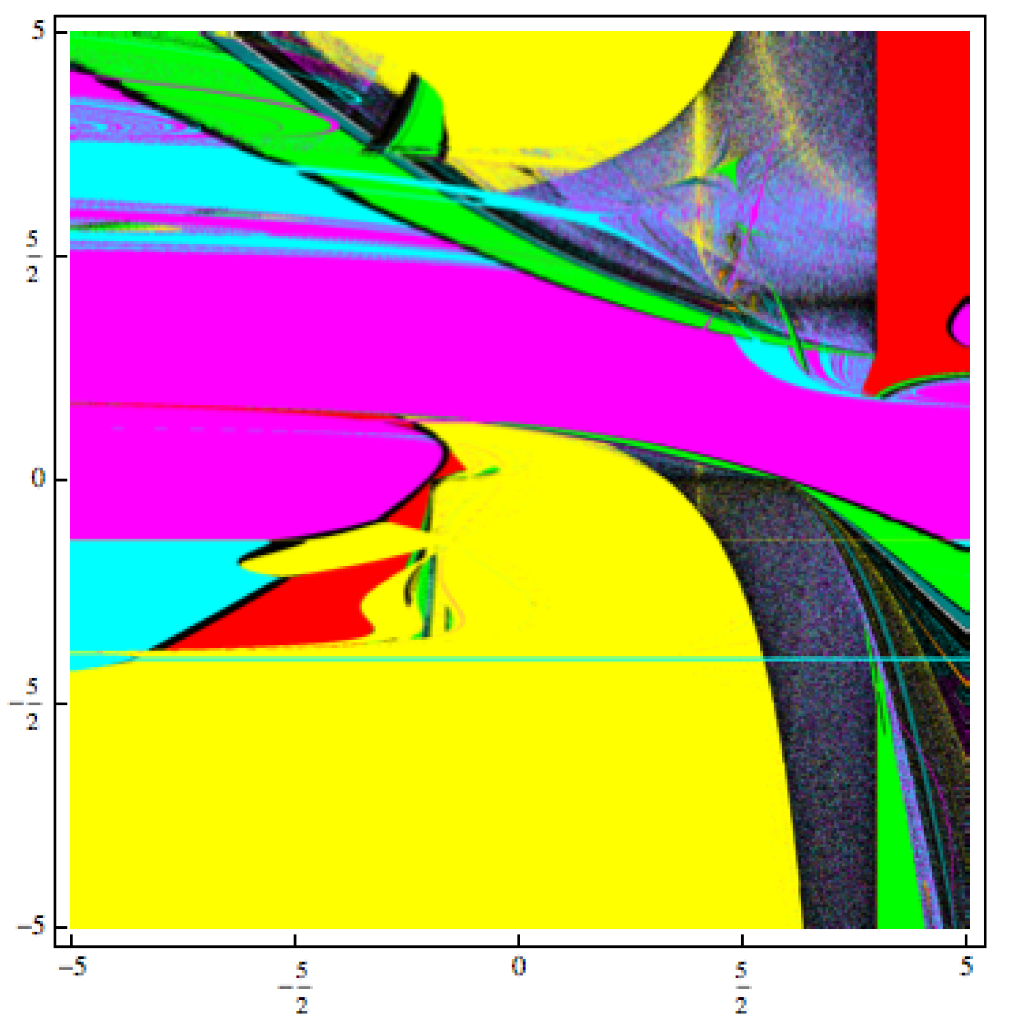
Abstract
1. Introduction
2. Local Convergence Analysis
- (a)
- (b)
- Concerning the second and the thirs conditions in Theorem 1, these were left as uncluttered as possible. One can easily see that there are infinitely many pair of values satisfying these inequalities (but not as weak). Indeed, suppose thatThen, the second inequality is satisfied provided thatorThen, the original inequalities certainly hold, if (27) and (28) hold. Moreover, (27) (in view of (28)) can ever be replaced byHowever as noted earlier condtions (27) and (28) or (28) and (29) are stronger than the two inequalities appearing in the statemetn of Theorem 1 (and can certainly replace them). Either way, as claimed above there are infinitely many choices of .
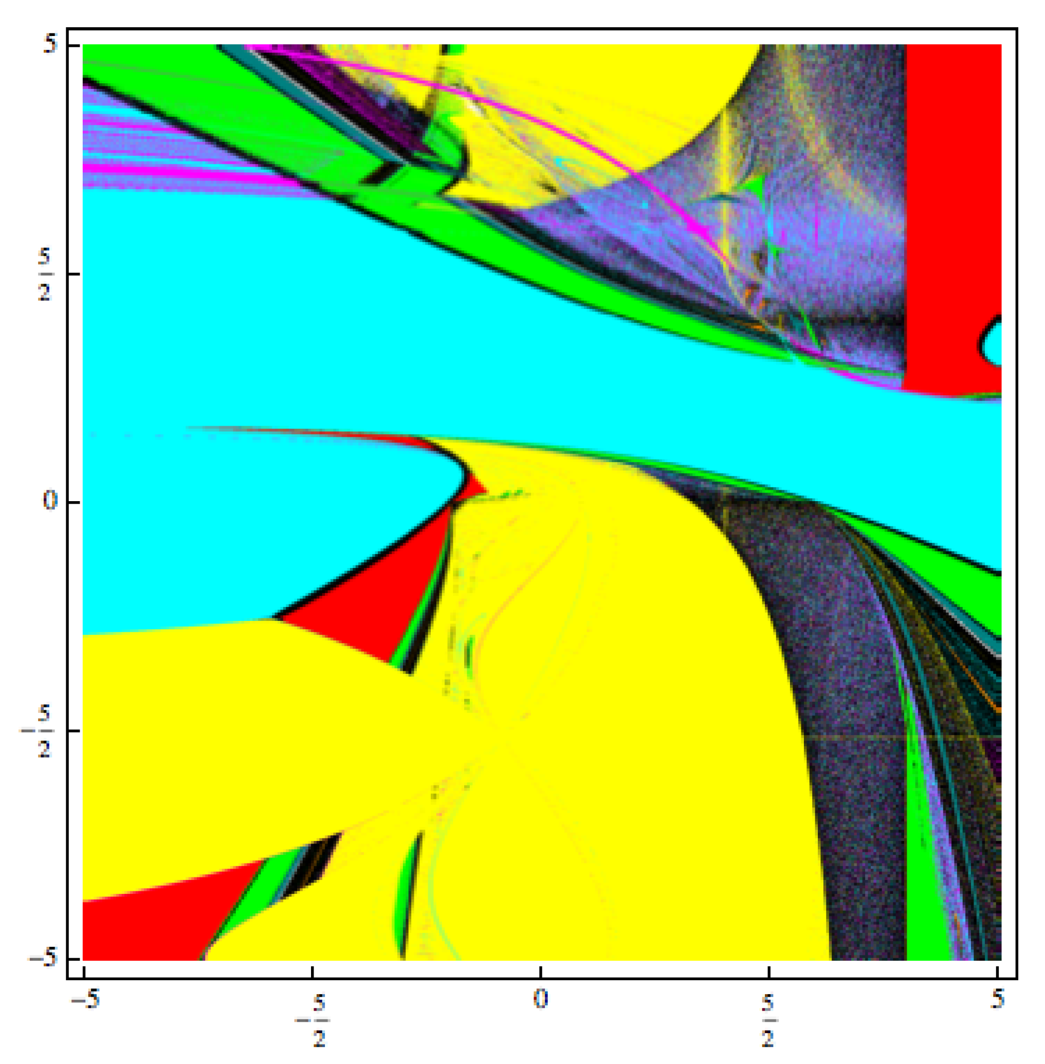
3. The Convergence Planes Applied to the Quadratic Polynomial Using Method (2)
- in yellow if the iteration of the initial point diverges to ∞,
- in magenta if the starting point converges to the first root of the quadratic polynomial, ,
- in cyan if the iteration of the starting point converges to the other root of the quadratic polynomial ,
- if the iteration of the initial point converges to any strange fixed points, it is colored in red,
- in other colors if the iteration of the initial point converge to different n-cycles (),
- in black if the iteration of the initial point has other behavior.
4. Application Examples
5. Conclusions
Author Contributions
Funding
Conflicts of Interest
References
- Magrenán, Á.A.; Argyros, I.K. Ball convergence theorems and the convergence planes of an iterative method for nonlinear equations. SEMA J. 2015, 71, 39–55. [Google Scholar] [CrossRef]
- Argyros, I.K. Convergence and Application of Newton-Type Iterations; Springer: Berlin, Germany, 2008. [Google Scholar]
- Argyros, I.K.; Hilout, S. Numerical methods in Nonlinear Analysis; World Scientific Publishing Company: Hackensack, NJ, USA, 2013. [Google Scholar]
- Traub, J.F. Iterative Methods for the Solution of Equations; Prentice- Hall Series in Automatic Computation; Englewood Cliffs: Bergen County, NJ, USA, 1964. [Google Scholar]
- Rall, L.B. Computational Solution of Nonlinear Operator Equations; Robert, E., Ed.; Krieger Pub. Co. Inc.: New York, NY, USA, 1979. [Google Scholar]
- Bruns, D.D.; Bailey, J.E. Nonlinear feedback control for operating a nonisothermal CSTR near an unstable steady state. Chem. Eng. Sci. 1997, 32, 257–264. [Google Scholar] [CrossRef]
- Amat, S.; Busquier, S.; Plaza, S. Dynamics of the King and Jarratt iterations. Aequationes Math. 2005, 69, 212–223. [Google Scholar] [CrossRef]
- Budzko, D.; Cordero, A.; Torregrosa, J.R. A new family of iterative methods widening areas of convergence. Appl. Math. Comput. 2015, 252, 405–417. [Google Scholar] [CrossRef]
- Amat, S.; Busquier, S.; Plaza, S. Chaotic dynamics of a third-order Newton-type method. J. Math. Anal. Appl. 2010, 366, 24–32. [Google Scholar] [CrossRef]
- Candela, V.; Marquina, A. Recurrence relations for rational cubic methods I: The Halley method. Computing 1990, 44, 169–184. [Google Scholar] [CrossRef]
- Candela, V.; Marquina, A. Recurrence relations for rational cubic methods II: The Chebyshev method. Computing 1990, 45, 355–367. [Google Scholar] [CrossRef]
- Chicharro, F.; Cordero, A.; Torregrosa, J.R. Drawing dynamical and parameters planes of iterative families and methods. Sci. World J. 2013, 2013, 780153. [Google Scholar] [CrossRef]
- Chun, C. Some improvements of Jarratt’s method with sixth-order convergence. Appl. Math. Comput. 1990, 190, 1432–1437. [Google Scholar] [CrossRef]
- Ezquerro, J.A.; Hernández, M.A. New iterations of R-order four with reduced computational cost. BIT Numer. Math. 2009, 49, 325–342. [Google Scholar] [CrossRef]
- Ezquerro, J.A.; Hernández, M.A. On the R-order of the Halley method. J. Math. Anal. Appl. 2005, 303, 591–601. [Google Scholar] [CrossRef]
- Gutiérrez, J.M.; Hernández, M.A. Recurrence relations for the super-Halley method. Comput. Math. Appl. 1998, 36, 1–8. [Google Scholar] [CrossRef]
- Ganesh, M.; Joshi, M.C. Numerical solvability of Hammerstein integral equations of mixed type. IMA J. Numer. Anal. 1991, 11, 21–31. [Google Scholar] [CrossRef]
- Hernández, M.A.; Salanova, M.A. Sufficient conditions for semilocal convergence of a fourth order multipoint iterative method for solving equations in Banach spaces. Southwest J. Pure Appl. Math. 1999, 1, 29–40. [Google Scholar]
- Kou, J.; Li, Y. An improvement of the Jarratt method. Appl. Math. Comput. 2007, 189, 1816–1821. [Google Scholar] [CrossRef]
- Kou, J.; Wang, X. Semilocal convergence of a modified multi-point Jarratt method in Banach spaces under general continuity conditions. Numer. Algorithms 2012, 60, 369–390. [Google Scholar]
- Li, D.; Liu, P.; Kou, J. An improvement of the Chebyshev-Halley methods free from second derivative. Appl. Math. Comput. 2014, 235, 221–225. [Google Scholar] [CrossRef]
- Ezquerro, J.A.; Hernández, M.A. Recurrence relations for Chebyshev-type methods. Appl. Math. Optim. 2000, 41, 227–236. [Google Scholar] [CrossRef]
- Magrenán, Á.A. Different anomalies in a Jarratt family of iterative root-finding methods. Appl. Math. Comput. 2014, 233, 29–38. [Google Scholar]
- Magrenán, Á.A. A new tool to study real dynamics: The convergence plane. Appl. Math. Comput. 2014, 248, 215–224. [Google Scholar] [CrossRef]
- Sarría Martínez de Mendivil, Í.; González Crespo, R.; González-Castanø, A.; Magrenán Ruiz, Á.A.; Orcos Palma, L. Herramienta pedagógica basada en el desarrollo de una aplicación informática para la mejora del aprendizaje en matemática avanzada. Rev. Esp. Pedagog. 2019, 274, 457–485. (In Spanish) [Google Scholar] [CrossRef]
- McNamee, J.M. A bibliography on roots of polynomials. J. Comput. Appl. Math. 1993, 47, 391–394. [Google Scholar] [CrossRef]
- McNamee, J.M. A supplementary bibliography on roots of polynomials. J. Comput. Appl. Math. 1997, 78, 1. [Google Scholar] [CrossRef]
- Mcnamee, J.M. An updated supplementary bibliography on roots of polynomials. J. Comput. Appl. Math. 1999, 110, 305–306. [Google Scholar] [CrossRef]
- Bartoň, M.; Jüttler, B. Computing roots of polynomials by quadratic clipping. Comput. Aided Geom. Des. 2007, 24, 125–141. [Google Scholar] [CrossRef]
- Sherbrooke, E.C. Computation of the solutions of nonlinear polynomial systems. Comput. Aided Geom. Des. 1993, 10, 379–405. [Google Scholar] [CrossRef][Green Version]
- Cordero, A.; Torregrosa, J.R. Variants of Newton’s method using fifth-order quadrature formulas. Appl. Math. Comput. 2007, 190, 686–698. [Google Scholar] [CrossRef]
- Divya, J. Families of Newton-like methos with fourth-order convergence. Int. J. Comput. Math. 2013, 90, 1072–1082. [Google Scholar]


© 2020 by the authors. Licensee MDPI, Basel, Switzerland. This article is an open access article distributed under the terms and conditions of the Creative Commons Attribution (CC BY) license (http://creativecommons.org/licenses/by/4.0/).
Share and Cite
Argyros, I.K.; Magreñán, Á.A.; Moysi, A.; Sarría, Í.; Sicilia Montalvo, J.A. Study of Local Convergence and Dynamics of a King-Like Two-Step Method with Applications. Mathematics 2020, 8, 1062. https://doi.org/10.3390/math8071062
Argyros IK, Magreñán ÁA, Moysi A, Sarría Í, Sicilia Montalvo JA. Study of Local Convergence and Dynamics of a King-Like Two-Step Method with Applications. Mathematics. 2020; 8(7):1062. https://doi.org/10.3390/math8071062
Chicago/Turabian StyleArgyros, Ioannis K., Ángel Alberto Magreñán, Alejandro Moysi, Íñigo Sarría, and Juan Antonio Sicilia Montalvo. 2020. "Study of Local Convergence and Dynamics of a King-Like Two-Step Method with Applications" Mathematics 8, no. 7: 1062. https://doi.org/10.3390/math8071062
APA StyleArgyros, I. K., Magreñán, Á. A., Moysi, A., Sarría, Í., & Sicilia Montalvo, J. A. (2020). Study of Local Convergence and Dynamics of a King-Like Two-Step Method with Applications. Mathematics, 8(7), 1062. https://doi.org/10.3390/math8071062