Article

Effect of a Boundary Layer on Cavity Flow

by
Yuriy N. Savchenko
1,
Georgiy Y. Savchenko
1 and
Yuriy A. Semenov
1,2,*
1
Institute of Hydromechanics of the National Academy of Sciences of Ukraine, 8/4 Zhelybova Street, 03680 Kiev, Ukraine
2
Department of Mechanical Engineering University College London, Gower Street, London WC1E 6BT, UK
*
Author to whom correspondence should be addressed.
Mathematics 2020, 8(6), 909; https://doi.org/10.3390/math8060909
Submission received: 23 March 2020 / Revised: 27 May 2020 / Accepted: 29 May 2020 / Published: 3 June 2020

Abstract

:
Cavity flow past an obstacle in the presence of an inflow vorticity is considered. The proposed approach to the solution of the problem is based on replacing the continuous vorticity with its discrete form in which the vorticity is concentrated along vortex lines coinciding with the streamlines. The flow between the streamlines is vortex free. The problem is to determine the shape of the streamlines and cavity boundary. The pressure on the cavity boundary is constant and equal to the vapour pressure of the liquid. The pressure is continuous across the streamlines. The theory of complex variables is used to determine the flow in the following subregions coupled via their boundary conditions: a flow in channels with curved walls, a cavity flow in a jet and an infinite flow along a curved wall. The numerical approach is based on the method of successive approximations. The numerical procedure is verified considering a body with a sharp edge, for which the point of cavity detachment is fixed. For smooth bodies, the cavity detachment is determined based on Brillouin’s criterion. It is found that the inflow vorticity delays the cavity detachment and reduces the cavity length. The results obtained are compared with experimental data.

1. Introduction

The theoretical study of cavity flows is usually based on the model of ideal liquid with the assumption that the liquid is incompressible, inviscid and irrotational. Liquid viscosity manifests itself in a thin boundary layer next to the body and can be ignored in the rest of the flow region. However, in some cases the boundary layer may develop far upstream due to interaction with other bodies situated upstream. In such cases the thickness of the boundary layer may be comparable with or exceed the size of the body that forms a cavity. In these cases the velocity profile of the inflow is nonuniform, which makes it difficult to introduce the velocity potential function.
The theoretical study of non-potential flows presents a great challenge and requires special treatments. The exception is flows with a constant vorticity, for which the velocity potential can be introduced in the form of a superposition of a potential vortex-free flow and a flow generated by a single vortex. Since the position and strength of the single vortex are prescribed, for the potential component of the flow the effect of the vortex can be accounted for through appropriate changes in the boundary conditions.
Cavity flows with a constant vorticity in a linear approximation were studied by Street [1], Vasil’iev [2], Kotlyar & Lazarev [3]. They formulated a boundary-value problem for the potential component of the flow and solved the boundary-value problem for the velocity potential function by using the Keldish-Sedov integral formula [4,5]. Kotlyar and Lazarev [3] presented a solution for a cavitating wedge in a flow with a uniform vorticity. The nonlinear problem of a cavity flow with a uniform vorticity for a wedge in a jet of finite width was considered in papers [6] and [7]. These studies revealed that the vorticity weakly affects the drag coefficient, but significantly decreases the cavity size.
In the cavity flows with vorticity mentioned above, the cavity detachment point is fixed at the body’s sharp edge. If the body is smooth, the location of the separation point is not known a priori and has to be determined as part of the solution of the problem. In the model of ideal liquid, flow detachment is governed by Brillouin-Villat’s criterion [8,9], from which it follows that the curvature of the free surface is equal to the body surface curvature at the point of detachment. At the same time, experiments [10,11,12] show that in a real liquid flow detachment occurs downstream of the point predicted by the model of ideal liquid. The real properties of the liquid such as viscosity or surface tension may affect the position of flow detachment [13]. In the present study, we investigate how the vorticity generated by the fluid viscosity in the boundary layer may affect the position of cavity detachment. For this purpose, we apply the methodology [7], which allows one to reduce the problem of a flow with a continuously distributed nonuniform vorticity to a set of problems of vortex-free potential flows related to one another via boundary conditions that account for the vorticity of the original flow.
The methodology is described in Section 2. The main idea is to replace a continuously distributed vorticity with discrete vortex sheets that coincide with the streamlines. In Section 3, solutions to the set of potential vortex free flows including the cavity flow past the body are presented. The effect of the velocity profile in the boundary layer on the cavity size and the force coefficient is analysed in Section 4. The numerical approach is comprehensively verified in Section 4.1, and the effect of the boundary layer on the cavity detachment is presented in Section 4.2.

2. General Approach for Flows with Vorticity

Fluid viscosity manifests itself in the boundary layer and causes a significantly nonuniform flow vorticity. The vorticity varies from zero on the outer boundary of the boundary layer to some value on the body boundary. In order to account for the non-uniformity of the vorticity, the continuously distributed vorticity in the flow region is replaced with discrete vortex sheets wherein the vorticity is concentrated. The vortex sheets are arranged along the streamlines, and the flow between the vortex lines is assumed to be vortex free. The flow region is divided into layers/channels bounded by the vortex sheets, or streamlines as shown in Figure 1. The normal components of the velocity and the pressure are continuous across the walls of the channels, while their tangential components are discontinuous. In this approach, the velocity profile changes in a stepwise manner from one channel to another. The larger the number of layers/channels, the smaller the stepwise discontinuity in the velocity profile, and it disappears in the limit of an infinite number of layers/channels. This corresponds to the original flow with a continuous nonuniform vorticity.
This vortex flow model allows one to reduce the problem of a cavity flow with a vorticity to a set of problems of vortexfree flows, which can be solved using the theory of potential flows. There are three kinds of vortex-free problems which constitute the original problem: the first kind is a cavity flow in a channel of finite width with a given shape of the lower side and a specified velocity distribution on the upper side (channel ‘0’ in Figure 1); the second kind is a flow in a channel with curved walls (channels 1 ÷ N ) ; and the third kind is a semi-infinite flow along a curved surface (layer N + 1 ) .
Each problem mentioned above is solved using the methods proposed by Michell [14], Joukovskii [15] and Chaplygin [16]. They introduced a parameter plane in which boundary value problems for both the complex velocity, d w / d z , and the derivative of the complex potential, d w / d ζ , are formulated. When these functions are determined, the mapping function relating the parameter plane and the physical plane is determined as follows
z ( ζ ) = z 0 + 0 ζ d z d ζ d ζ = z 0 + 0 ζ d w d ζ / d w d z d ζ ,
where z 0 is the point in the physical plane corresponding to the point ζ = 0 in the parameter plane.
The singular point method developed by Chaplygin (see Section 1 in [16]) allows one to derive expressions for the complex velocity and the derivative of the complex potential when the solid boundary forms a polygon, and the velocity on the free surface is constant. The problems under consideration are somewhat more complicated. One part of the flow boundary is considered as a solid curved wall, and the other part is a free streamline along which the velocity magnitude may vary. For this kind of boundary value problem, the solution can be obtained using the integral formula derived in [17,18]. The formula and details of its application are shown in Section 2.
The set of problems mentioned above is solved successively as follows. By solving the problem for the zeroth channel in which the cavity occurs as shown in Figure 1, the shape of the upper wall is determined assuming the velocity magnitude to be known from the previous iteration. This wall, which is also the lower side of channel 1, is considered as a solid wall in channel 1. The upper wall of channel 1 is considered as a free streamline, along which the velocity magnitude is assumed to be known from the previous iteration. By solving the problem for channel 1 the shape of its upper side is determined. By repeating the process we can arrive at the outer layer N + 1 corresponding to the half-space of the liquid flowing along the curved solid wall of channel N. By solving this problem, the velocity magnitude on the upper wall of channel N can be determined.
Now we start moving back and solving the problem for channel N, we can find a new approximation of the velocity distribution along the lower side of channel N. Using the condition of pressure continuity across the channels, we can obtain a new approximation of the velocity distribution on the upper side of channel N 1 . Moving down and repeating the procedure for each channel, we can specify the velocity magnitude on the upper side of the zeroth channel. The successive computations in the up and down directions are repeated until the convergence of the iteration process. Notice that the computational efficiency depends on the effective solution procedure for each channel from 0 to N. The solutions of the flow problems in the channels are presented in next section.

3. Complex Potentials of Flows

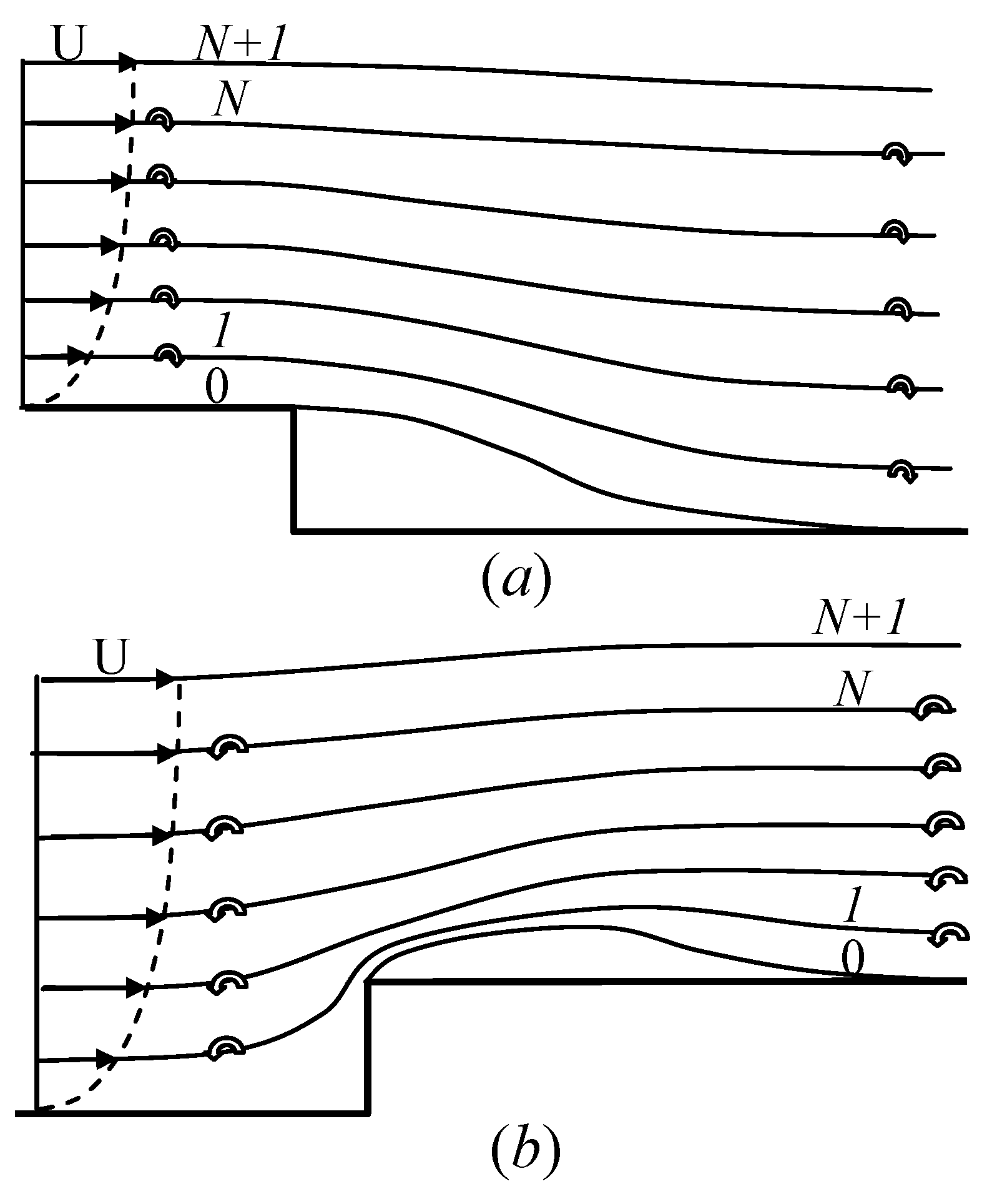
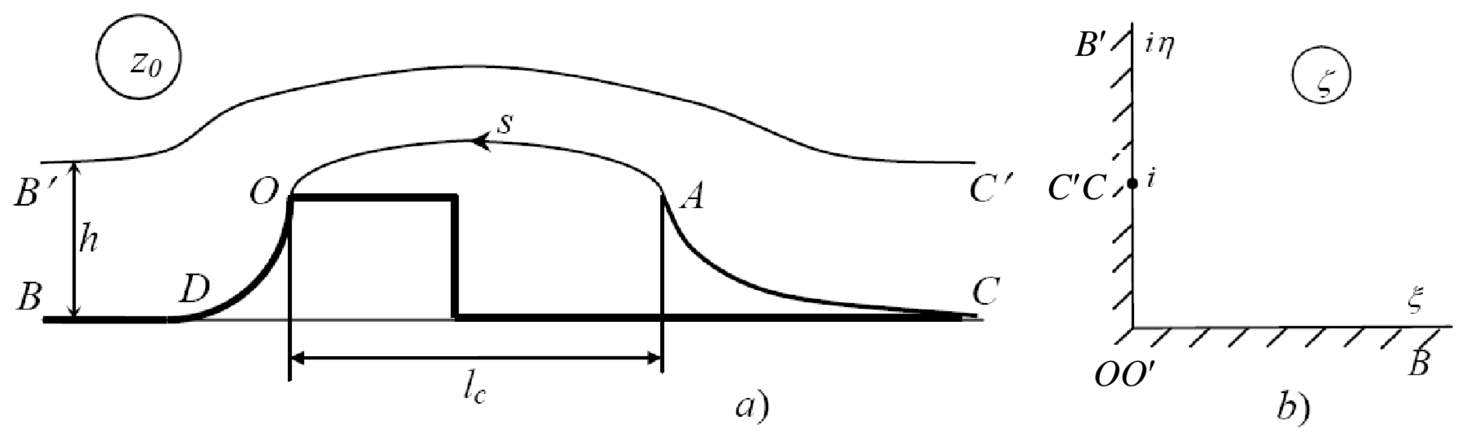
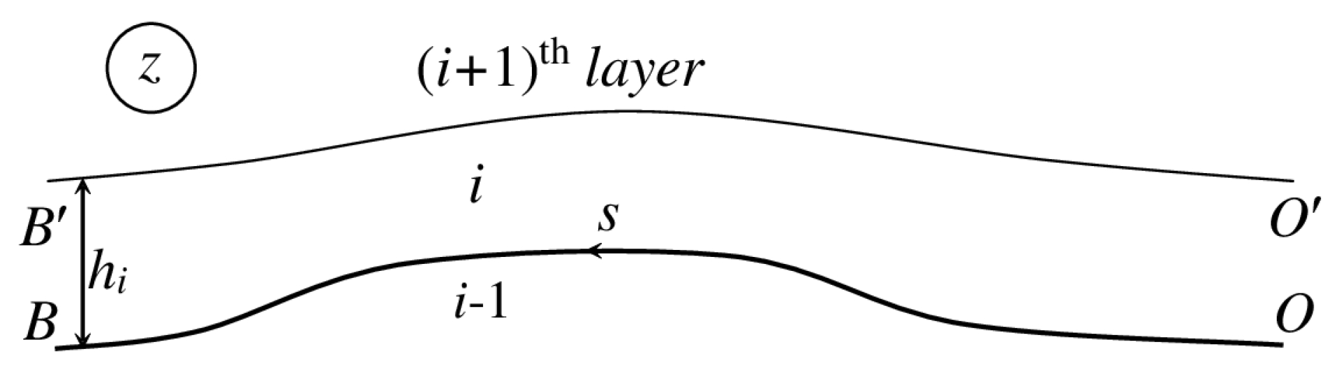
3.1. Cavity Flow in Channels with Curved Walls

Figure 2 shows a schematic of the “zeroth” channel with the cavity. For convenience, the channel number subscript is omitted. The liquid is assumed to be ideal, incompressible and irrotational. The pressure on the cavity surface O A is assumed to be constant and equal to the pressure in the cavity p c . The origin of the Cartesian coordinate system x y is chosen at point O where the flow detaches from the body and forms the cavity contour O A . The flow velocity at infinity, B B , is V. The shape of the obstacle D O is given by its slope β * ( s ) where s is the arc length coordinate along the contour. On the contours A C and B C the velocity magnitude is specified, v * ( s ) . The cavity contour O A closes on the contour A C , along which the velocity magnitude decreases from its value on the cavity boundary to its value at infinity, C C . The pressure at infinity is the same in all directions, therefore the velocity at right infinity is also V. The cavity contour O A , the closure contour A C and the upper wall B C are unknown. They have to be determined from the solution of the problem.
We introduce a cavitation number σ 0 based on the reference velocity V in the channel and a cavitation number σ based on the velocity on the outer boundary of the boundary layer, U, which are related as follows
σ 0 = p p c 0.5 ρ V 2 , σ = p p c 0.5 ρ U 2 , σ 0 = σ v 2 ,
where v = V / U is the dimensionless incident velocity. Based on these definitions, the velocity on the cavity surface is v 0 = v 1 + σ 0 .
The problem is solved in the parameter plane. The first quadrant of the ζ -plane is chosen as the parameter region that corresponds to the flow region in the physical plane z. The conformal mapping theorem allows us to chose the position of three points in the parameter region arbitrarily. They are O, B and C as shown in Figure 2b.
The real axis in the ζ -plane corresponds to the solid body B D O . The interval 0 < η < 1 of the imaginary axis corresponds to the cavity contour O A and the cavity-closure contour A C . The interval 1 < η < corresponds to the upper side of the channel, B C . We assume that the velocity magnitude v * ( s ) on the upper side B C is known. It will determined later in the iterative solution of the whole problem.
In order to derive an expression for the complex velocity, d w / d z , we assume that the velocity magnitude on the contours O A C and B C is known as a function of the parameter variable η , v ( η ) . We also assume that the slope of the solid surface O D B is known as a function of the variable ξ , β ( ξ ) . Then, we can write the following boundary-value problem for the complex velocity function:
d w d z = v ( η ) , 0 < η < , ξ = 0 .
χ ( ξ ) = arg d w d z = β ( ξ ) , 0 < ξ < d , η = 0 , 0 , d < ξ < , η = 0 .
The functions v ( η ) and β ( ξ ) will be determined later.
The integral formula [18]
d w d z = v ( ) exp 1 π 0 d χ d ξ ln ζ + ξ ζ ξ d ξ i π 0 d ln v d η ln ζ i η ζ + i η d η + i χ ( ) ,
provides a solution to the mixed boundary-value problem in Equations (3) and (4). Here, v ( ) = v ( η ) η = is the velocity magnitude at infinity B B . It can be easily verified that for ζ = ξ the argument of the function d w / d z is the function χ ( ξ ) , while for ζ = i η the modulus | d w / d z | is the function v ( η ) . Thus, the boundary conditions in Equations (3) and (4) are satisfied. Substituting Equation (4) into the first integral and using the relation arg ( ζ i η ) = arg ( i η ζ ) π in the second integral, we obtain the following expression for the complex velocity
d w d z = v 0 exp 1 π 0 d β d ξ ln ζ ξ ζ + ξ d ξ i π 0 d ln v d η ln i η ζ i η + ζ d η i β 0 ,
where β 0 = β ( 0 ) is the angle of the velocity at point O, and
v 0 = v ( ) exp 0 d ln v d η d η
The complex flow potential has logarithmic singularities due to a sink at point C ( ζ = i ) and a source of the same strength at point B ( ζ = ) . By applying Chaplygin’s singular point method [16], we can obtain the derivative of the complex potential
d w d ζ = M ζ ζ 2 + 1 , w ( ζ ) = q π ln ζ 2 + 1 ,
where M = 2 q / π is a scale factor. By substituting Equations (6) and (7) into Equation (1), we obtain the derivative of the mapping function z = z ( ζ ) ,
d z d ζ = M v 0 ζ ζ 2 + 1 exp 1 π 0 d β d ξ ln ζ ξ ζ + ξ d ξ + i π 0 d ln v d η ln i η ζ i η + ζ d η + i β 0 .
The arc length coordinate along the free streamline, s = s ( η ) , and along the solid surface, s = s ( ξ ) , are obtained as follows
s ( η ) = 0 η d z d ζ ζ = i η d η , s ( ξ ) = 0 η d z d ζ ζ = ξ d ξ .

3.1.1. Cavity Closure Model

Within the framework of the model of ideal liquid, the statement of the cavity flow problem is not unique. This issue is known as Brillouin’s paradox [8], and it requires an assumption about the cavity contour at the end of the cavity. Various models were proposed by Roshko, Riabouchinsky, Efros, Tulin, and they are known as classical models of cavity flows [16,19]. These models predict similar results for developed cavitation regimes, for which the cavity exceeds the size of the body. When the size of the cavity is comparable with or smaller than the size of the body, the assumption may affect the results. This is because the cavity closure region becomes larger than the cavity itself.
Crocco and Lees [20] proposed a model of viscous/inviscid interaction for separated turbulent flows, which accounts for the effect of the viscous wake on the outer inviscid flow in real flows. Crocco and Lees’s [20] approach was extended to cavity flows (Semenov and Tsujimoto [21]), which made it possible to account for a turbulent wake downstream of the cavity. This model predicts a monotonic decrease in the velocity magnitude along the turbulent wake region from the velocity on the cavity boundary to the velocity at downstream infinity.
In the this paper we focus our attention on the effect of the vorticity, therefore, we drop the viscous wake model and assume a velocity distribution along the cavity closure region. For simplicity, we assume that the magnitude of the velocity v * ( s ) on the contour A C is the same as the velocity on the body O D B , i.e.,
v * [ s ( η ) ] = v [ s A s ( η ) ] = d w d z ζ = ξ 1 [ s A s ( η ) ] , s A < s < , η A < η < 1 .
These equations define the function v * ( s ) , which is symmetric about the middle cross section of the cavity at s = s A / 2 where s A is the arc length coordinate of point A. This definition of the velocity in the cavity closure region results in a flow pattern geometry symmetric about the vertical cross section passing through the point s = s A / 2 .
Notice that various classical cavity models can be obtained from the presented solution if the velocity magnitude along the cavity closure contour is chosen appropriately. For example, Tulin’s second cavity closure model [22] can be obtained as follows. Let the velocity magnitude at the cavity closure point change by step
v ( η ) = v 0 , 0 < η < η A , v , η A < η < 1 .
By substituting this Equation into Equation (6) and evaluating the second integral over the step change at point A ( η = η A )
lim ε 0 η A ε η A + ε d ln v d η ln i η ζ i η + ζ d η = ln i η A ζ i η A + ζ ln v v 0 ,
the complex velocity in Equation (6) takes the form
d w d z = v 0 i η A ζ i η A + ζ i π ln v 0 v exp 1 π 0 d β d ξ ln ξ ζ ξ + ζ d ξ i β 0 ,
The above expression is the complex velocity for the present problem corresponding to Tulin’s second cavity model.

3.1.2. Integro-Differential Equations in the Functions v ( η ) and β ( ξ )

The integro-differential equations determining the functions d ln v / d η and d β / d ξ are obtained using the chain rule for differentiation
d ln v d η = d ln v * d s d s d η , d β d ξ = d β * d s d s d ξ .
The functions v * ( s ) and β * ( s ) are known functions in the physical plane. The above equations are solved using the method of successive approximations.
d ln v d η k + 1 = d ln v * d s d s d η k , d β d ξ k + 1 = d β * d s d s d ξ k .

3.2. Jet Flow Along a Curved Wall

The flow in the channel next to the cavity channel is considered as a jet flow along the solid wall whose shape is obtained from the solution of the problem in channel 0 . A flow sketch is shown in Figure 3. The complex velocity function and the derivative of the potential are derived in the parameter plane which is chosen to be the same as that shown in Figure 2b. Point C is absent in the present case. Points O, O , B, B in Figure 3 correspond to the same points in the parameter plane in Figure 2b.
The velocity magnitude along the upper streamline is specified, and it is denoted v * ( s ) . The slope of the lower solid wall is denoted as β * ( s ) . The corresponding functions in the parameter plane are v ( η ) and β ( η ) . The boundary value problem for the complex velocity, d w / d z can be formulated as follows. The argument of the complex velocity is given along the real axis, arg ( d w / d z ) = β ( ξ ) , and its modulus is given along the imaginary axis of the parameter region, | d w / d z | = v ( η ) . Then, the integral formula in Equation (5) determines the complex velocity function as follows
d w d z = v exp 1 π 0 d β d ξ ln ζ ξ ζ + ξ d ξ i π 0 d ln v d η ln ζ i η ζ + i η d η ,
where v = V / U is the dimensionless velocity at left infinity (point B B ).
The complex potential for a jet of finite width has logarithmic singularities corresponding to a source at point B B ( ζ = ) , and to a sink of the same strength at point O O ( ζ = 0). Therefore, we can write
w ( ζ ) = 2 q π ln ζ , d w d ζ = 2 q π 1 ζ ,
where q = V h is the strength of the source/sink corresponding to the flow rate in the channel.
In view of Equation (1), the derivative of the mapping function takes the form
d z d ζ = 2 q π v exp 1 π 0 d β d ξ ln ζ ξ ζ + ξ d ξ + i π 0 d ln v d η ln ζ i η ζ + i η d η
By integrating Equation (15) along the imaginary axis of the parameter region we obtain the contour of the upper streamline of the jet. The functions v ( η ) and β ( ξ ) are obtained from the solution of integro-differential equations similar to Equation (12). The arc length coordinates along the solid surface, s = s ( ξ ) , and along the upper streamline, s = s ( η ) , are obtained from Equation (9).

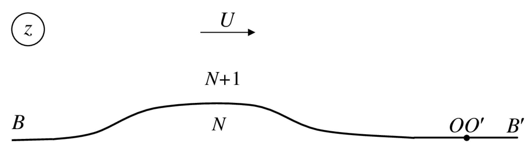
3.3. Semi-Infinite Flow Passing over a Solid Curved Surface

Layer N + 1 in Figure 1 occupies all the space of the upper half-plane. A sketch of the physical plane is shown in Figure 4. The position of points O, O , B and B is chosen so that they correspond to the same points in the parameter plane shown in Figure 2b. Points B and B are placed on the straight part of the solid surface far downstream, along which the velocity magnitude is constant and equal to the velocity at infinity.
Following Joukowskii’s method [16], we can obtain the complex potential in the form
d W d ζ = M ζ ,
where M is a scale factor.
The complex velocity is obtained from the integral formula in Equation (8) taking into account that d ln v / d η = 0 on the imaginary axis of the parameter region, i.e., the second integral in Equation (8) vanishes. The expression for the complex velocity takes the form
d w d z = v exp 1 π 0 d β d ξ ln ξ ζ ξ + ζ d ξ .
The derivative of the mapping function, d z / d ζ , is obtained from Equation (1) and Equations (16) and (17). The arc length coordinate s = s ( ξ ) is obtained from Equation (9).

4. Results and Discussion

The intgro-differential equations for each channel in Equation (12) are solved numerically using the method of successive approximations. Two sets of nodes are chosen on the real and the imaginary axis of the parameter region: ξ i , i = 1 , K ξ and η j , j = 1 , K η . On each interval ( ξ i 1 , ξ i ) and ( η j 1 , η j ) the derivatives d β / d ξ and d ln v / d η are assumed to be constant, which allows one to evaluate the integrals in Equations (6) and (8) analytically, thus significantly reducing the computational effort. Usually, from 10 to 15 iterations are required to reach the convergence of the iterations with a tolerance of 10 5 between successive iterations. The number of the nodes on the upper and the lower side of the channel is chosen to be K ξ = 200 and K η = 200 .

4.1. Cavity Flow with a Fixed Point of Cavity Detachment

The dimensionless velocity profile in the boundary layer is approximated by the function
v ( y ) = V ( y ) U = y δ 2 y δ , 0 y δ , 1 , δ y < ,
where U is the velocity on the outer boundary of the boundary layer, and δ is the boundary layer thickness. The flow rate and the inflow velocity in the channel i in view of Equation (18) are defined as follows
q i = 1 U L y i y i + 1 V ( y ) d y , v i = q i h i ,
where h i = ( y i + 1 y i ) / L is the width of channel i at infinity B B , and L is the length of the arc O D .
The interaction between adjacent channels accounts for the conditions of velocity direction and pressure continuity across the channel walls.
γ i 1 = β i , p i 1 u p = p i l w ,
where γ i 1 = arg d z / d η i 1 is the slope of the upper side of the channel i 1 , β i is the slope of the solid lower side of the channel i and p i 1 u p , p i l w are the pressures on the upper side of channel i 1 and the lower side of channel i, respectively.
From the Bernoulli integral for the adjacent channels
p + ρ U 2 v ( i 1 ) 2 2 = p i 1 u p + ρ U 2 v i 1 2 2 ,
p + ρ U 2 v i 2 2 = p i l w + ρ U 2 v i 2 2 ,
we can obtain the relation between the velocity magnitudes on the upper side of channel i 1 and on the lower side of channel i using Equation (19),
v i 1 2 u p = v i 2 l w + v i 1 2 v i 2 .
In the case of a uniform inflow, v i 1 = v i and v i 1 u p = v i l w . For the purpose of verification and accuracy estimation of the results, we divide the uniform jet of width H / L = 3 into jets of widths h 0 = H 0 / L = 1 and h 1 = H 1 / L = 2 . The cavity length is chosen to be s A / L = 2 , and the corresponding cavitation number is determined from the solution. Figure 5 shows the computed upper boundary of the flow for the two channels (solid line) and for the one channel (dashed line). The obtained cavitation number σ = 1.810 for the two channels and σ = 1.813 for the one channel demonstrates quite a good accuracy of the method.
The capability of the method to capture the effect of a nonuniform inflow velocity depends on the required discretization of the boundary layer. As the number of channels increases, the results should converge to those corresponding to the continuous inflow velocity profile.
Figure 6 shows the effect of the number of channels N on the cavitation number corresponding to cavity length s A / L = 2 and a linear velocity profile in the boundary layer. The results show that a 4- or 5-channel discratization of the boundary layer can provide results close to those corresponding to the continuous velocity profile in the boundary layer. It can also be seen that the boundary layer thickness has a weak effect on the required number of discrete channels.
The effect of the boundary layer thickness on the streamline shape and the cavity size is shown in Figure 7a,b for a parabolic velocity profile (Equation (18)). It can be seen that the cavity length becomes smaller as the boundary layer thickness increases. This is because the velocity and thus the total flow pressure in the vicinity of the body decrease, which is similar to a greater local cavitation number.
The pressure coefficient can be derived using Equation (20) relating the outer inviscid flow and channel ‘0’ with the cavity
c p = p p 1 2 ρ U 2 = v 0 2 + σ v 2 ,
where v 0 and v are the velocity at infinity and on the body in channel ‘0’, respectively. Then, the drag force coefficient is defined as
C x = 1 h b 0 d c p s ( ξ ) sin β s ( ξ ) d s d ξ d ξ ,
where the height of the body is h b = 0 L sin β ( s ) d s , and d is the coordinate of point D on the real axis of the parameter region (see Figure 2).
The drag coefficient versus the relative thickness of the boundary layer is shown in Figure 8. The results correspond to a linear velocity profile of the incoming flow at infinity. It can be seen that for boundary layer thickness δ / L > 0.5 , the cavitation number and the drag coefficient are nearly the same. This is because the contribution of the dynamic component to the total pressure is small. As the boundary layer thickness tends to zero, the cavitation number and the drag coefficient tend to their values corresponding to potential vortex-free flow past the arc of circle.

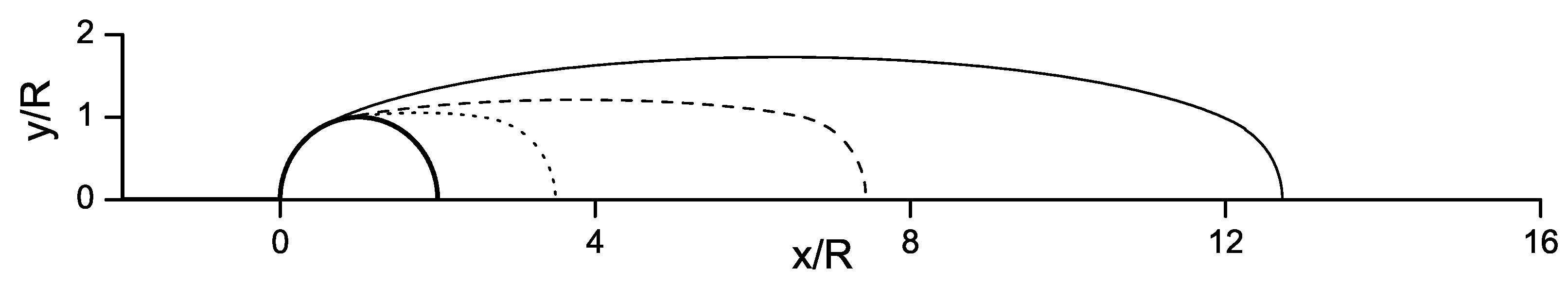
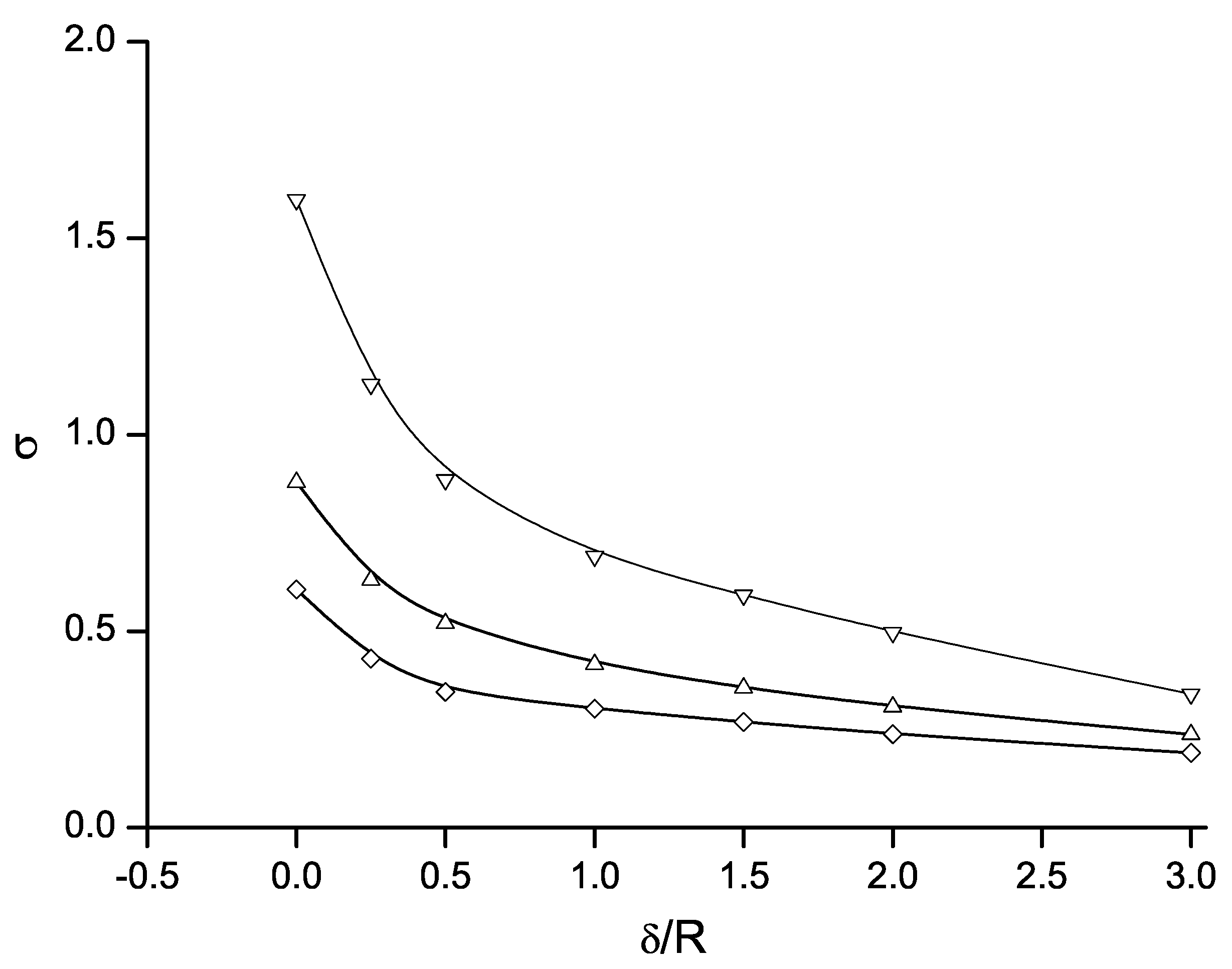
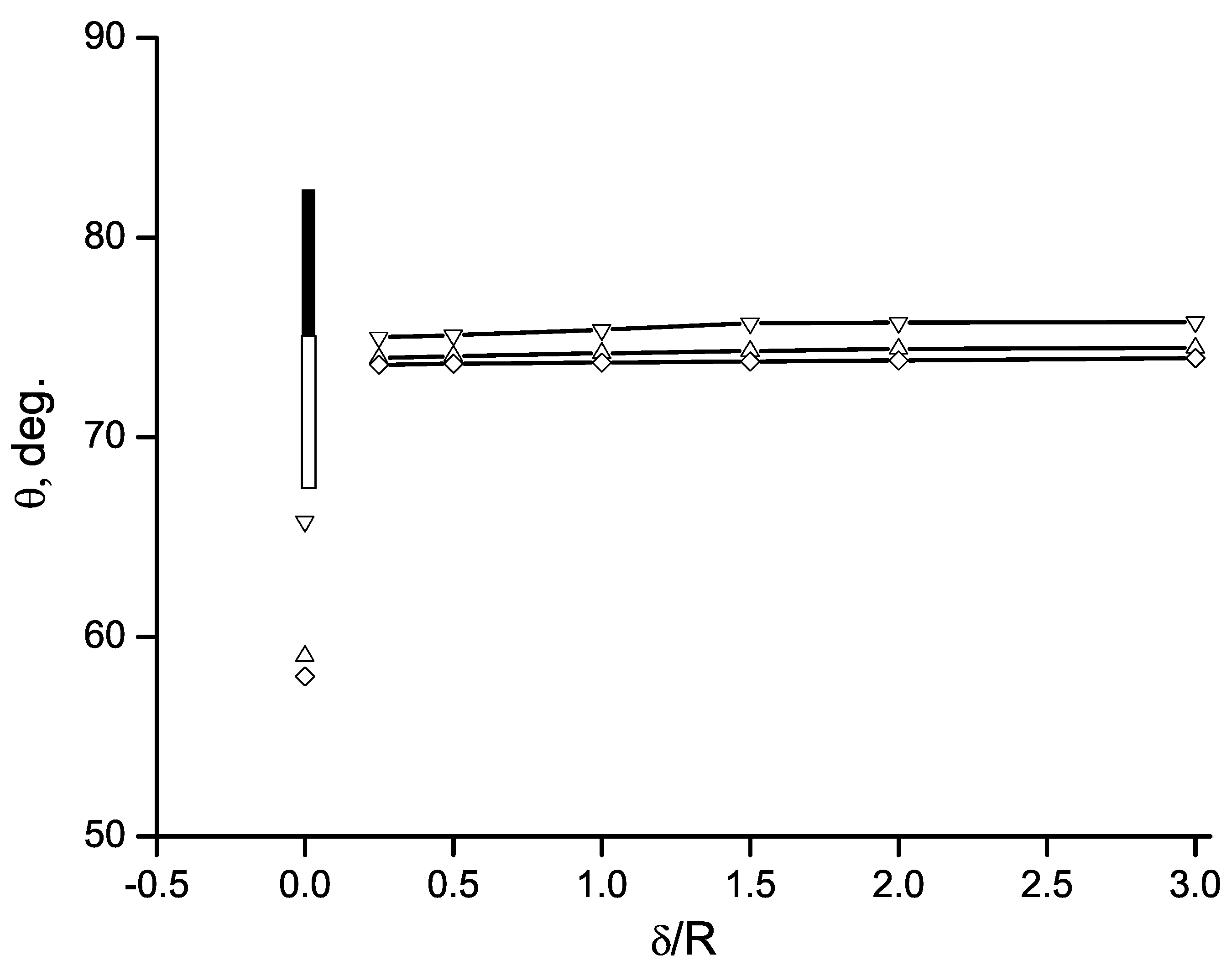
4.2. Cavity Flow Past a Circular Cylinder

For a body with a sharp edge, the pressure takes its minimal value at the edge, which leads to cavity inception. Therefore, the position of cavity detachment is fixed at that point. For smoothly shaped bodies, the position of the minimal pressure is unknown, and it has to be determined as part of the solution of the problem. In the model of ideal liquid, cavity detachment is determined from Brillouin-Villat’s criterion [8,9], which states that the cavity detaches tangentially to the solid surface and the curvature of the free surface is equal to the curvature of the body at the detachment point. These conditions lead to the equation derived by Villat [9],
lim s 0 d v d s = lim s 0 d d s d w d z ζ = 0 = 0 ,
where s is the arc length along the wetted part of the body. The physical meaning of this equation is that the velocity in the flow region reaches its maximal value at the detachment point.
We apply the presented method to the study of the effect of the boundary layer on cavity flow past smoothly shaped bodies. According to the model, the flow in the channels is vortex free, and thus we can use Brillouin-Villat’s criterion [8,9] for the zeroth channel, where the cavity occurs. In view of Equation (6), Equation (22) takes the form
0 d β d ξ d ξ ξ + 0 d ln v d η d η η = 0 .
Equation (23) determines the position of point O ( ζ = 0 ), which influences the function β ( ξ ) = β [ s ( ξ ) ] .
Figure 9 shows cavity contours at different thicknesses of the boundary layer with the velocity profile of (18). The solid line corresponds to the case without boundary layer. It can be seen that the boundary layer significantly affects the size of the cavity. In addition, the position of the cavity detachment moves somewhat downstream. This feature will be discussed in the following.
The effect of the boundary layer on the cavitation number is shown in Figure 10 for different cavity lengths, s A / R . The cylinder radius R is chosen as the characteristic length. The results are similar to those shown in Figure 8 for the arc of circle with a fixed position of cavity detachment. The larger the thickness of the boundary layer, the smaller the cavitation number. This implies that a lower pressure at infinity is required to maintain the same cavity size.
Cavity detachment from smooth shaped bodies was studied experimentally by Arakeri and Acosta [10], Arakeri [11], Tassin-Leger and Ceccio [12]. These researches revealed that the real liquid properties such as viscosity, surface tension and the solid/liquid work of adhesion affect the cavity detachment position. Among these physical properties, the liquid viscosity plays the major role due to the development of a boundary layer on the body surface. Arakeri and Acosta [10] showed that viscous effects are predominant, and the mechanisms of cavity detachment and laminar boundary layer separation are related. A boundary layer separates first and foremost due to an adverse pressure gradient of the external flow, and this determines the cavity detachment position. A recirculation region may occur between the points of laminar boundary layer separation and cavity detachment. Its size may vary significantly depending on the flow configuration, surface tension and the solid/liquid work of adhesion. Sometimes, this region is not observed in experiments [23].
The present model does not account for the flow viscosity, but it can account the effect of the boundary layer, which has been developed at upstream. The angle of cavity detachment, θ , measured from the front stagnation point is shown in Figure 11 as function of the thickness of the boundary layer at upstream, δ / R , for different cavity lengths or the cavitation numbers. The smallest thickness of the boundary layer for which the results were obtained is δ / R = 0.25 . For the smaller thickness of the boundary layer, the larger number of nodes ξ i , i = 1 , K ξ and η j , j = 1 , K η is necessary to capture the same size of the flow region in the physical plane.
In Figure 11 it can be seen that the angle θ remains nearly constant in the wide range of the boundary layer thickness from δ / R = 0.25 to 3.0 . The cavity length, (the cavitation number) also weakly affects the position of cavity detachment. By contrast, the angle θ predicted by the model of ideal liquid without a boundary layer, δ = 0 , is smaller, and it depends on the cavity length. These results are shown as open symbols on the y-axis for different cavity lengths. As the cavity length decreases, the angle θ increases, i.e., the position of cavity detachment moves slightly downstream.
The angles θ of laminar flow separation and cavity detachment were measured in Tassin-Leger and Ceccio [12] for a cavitating cylinder in a uniform flow for the range of Reynolds numbers from 6 × 10 4 to 3 × 10 5 and for cavitation numbers σ = 1.1 and 1.3 . There is no upstream boundary layer for this case, i.e., δ = 0 . A very thin boundary layer develops on the wetted part of the cylinder surface for this range of Reynolds numbers, which does not affect the outer flow. The angles of laminar separation and cavity detachment measured in those experiments are shown in Figure 11 as open and solid rectangles, respectively. We note that in those experiments, the position of laminar separation does not depend on the Reynolds number, while the angle of cavity detachment slightly decreases as the Reynolds number increases. Since the boundary layer thickness is very small for the Reynolds numbers in the range mentioned above, it does not affect the outer flow, which determines the pressure gradient along the wetted surface of the cylinder and, accordingly, the separation of the laminar boundary layer.
By comparing the predicted angle of cavity detachment θ with the experimental data, we can see that the predicted values of the angle θ are in the middle of the range that includes both the separation of the laminar boundary layer and the cavity detachment measured in the experiments. The results obtained can be justified based on the model of ideal liquid, whose results are shown in Figure 11 as open symbols. The smaller the cavity length (the larger the cavitation number), the larger the angle of cavity detachment. In the presence of a boundary layer, the angle θ is governed by the local cavitation number σ 0 for the zeroth channel rather than the cavitation number σ for the whole flow. As a result that σ 0 based on the average velocity V in the zeroth channel is larger than σ based on the velocity U of the outer inflow, the angle θ ( σ 0 ) in the presence of a boundary layer is larger than θ ( σ ) without a boundary layer. Although the model developed does not include the physical properties of the liquid directly, the inclusion of the boundary layer into consideration provides relatively good agreement of the cavity detachment with the experimental data.

5. Conclusions

A general approach to the solution of steady cavity flows in the presence of an inflow vorticity is presented. The approach is based on replacing the continuously distributed vorticity with discrete vortex lines placed along the streamlines. This allows one to dispense with solving Poisson’s equation. The flow between the vortex lines is assumed to be vortex free, thus making it possible to formulate boundary value problems for the velocity potential in the vortex free subregions.
A set of potential flow problems coupled via boundary conditions is formulated. They include a cavity jet flow past an arbitrary shaped body, a flow in curved channels and an unbounded flow along a curved wall. These boundary value problems are solved using the integral hodograph method to determine the complex velocity and the derivative of the potential in explicit form as a function of the parameter variable. The derived system of integro-differential equations in the velocity magnitude and the velocity angle on the boundary of the flow regions is solved numerically using the method of successive approximations. The convergence and accuracy of the computations are comprehensively verified by comparing the potential flow in the whole flow region and its subregions formed by the streamlines.
The presented method allows one to account for a nonuniform vorticity of the inflow and study the effect of the boundary layer on the cavity size, the force coefficient, and the flow detachment position for smoothly shaped bodies. The results obtained show that the boundary layer reduces the size of the cavity and the force coefficient. The larger the boundary layer thickness, the smaller the cavity size and the drag coefficient. When the boundary layer thickness is greater than the height of the obstacle, the dynamic term in the Bernoulli equation contributes to the drag coefficient to a far smaller extent than the static pressure. This agrees with the results obtained, which show that the drag coefficient is nearly equal to the cavitation number.
The analysis of cavity flows past smoothly shaped bodies revealed the effect of the boundary layer on the cavity detachment position. The effect is associated with the momentum of the liquid near the surface of the body. As the velocity near the body surface decreases, the local cavitation number increases, as a result of which the position of cavity detachment slightly moves downstream as predicted by the model of ideal liquid.
At the same time, the proposed model has numerical limitations in dealing with very thin boundary layers, and it does not account explicitly for viscosity, surface tension or the solid/liquid work of adhesion.

Author Contributions

Conceptualisation, Y.N.S. and Y.A.S.; methodology, G.Y.S. and Y.A.S.; software, Y.A.S. and G.Y.S.; validation, Y.N.S., G.Y.S. and Y.A.S.; formal analysis, Y.A.S.; investigation, Y.N.S., G.S. and Y.A.S.; resources, Y.N.S.; data curation, Y.N.S.; writing—original draft preparation, G.Y.S. and Y.A.S.; writing—review and editing, Y.A.S.; visualisation, Y.N.S. and G.Y.S.; supervision, Y.N.S.; project administration, Y.N.S.; funding acquisition, Y.N.S. All authors have read and agreed to the published version of the manuscript.

Funding

This research received no external funding.

Conflicts of Interest

The authors declare no conflict of interest.

Nomenclature

x , y Cartesian coordinates
z = x + i y Complex coordinate/physical plane
ζ = ξ + i η parametric variable/parameteric plane
sarclength coordinate
ϕ flow potential
ψ stream function
wcomplex potential
d w / d z complex velocity
d w / ζ derivative of the complex potential
ζ complex potential
H i width of the channel i
Lcharacteristics length
Rradius of the cylinder
p pressure at infinity
p c pressure in the cavity
Uvelocity on the outer boundary
Vaverage velocity across the channels
σ cavitation number based on U
σ 0 cavitation number based on V
vvelocity magnitude
β slope of the side of the channel
δ thickness of the boundary layer

References

  1. Street, R.L. A linearized Theory for Rotational Super-Cavitating Flow. J. Fluid Mech. 1963, 17, 513–545. [Google Scholar] [CrossRef] [Green Version]
  2. Vasiliev, V.N. Cavity vortex flow past a curved arc. In Unsteady Motion of Bodies in Liquid; University of Chuvashia: Cheboksary, Russia, 1979; pp. 3–15. [Google Scholar]
  3. Kotlyar, L.M.; Lazarev, V.A. Cavity vortex flow past a wedge. In Proceedings of the Boundary-Value Problem Workshop; Kazan’ State University: Kazan, Russia, 1971; pp. 15–25. [Google Scholar]
  4. Sedov, L.I. Plane Problems in Hydrodynamics and Aerodynamics; Nauka: Moscow, Russia, 1980; p. 448. [Google Scholar]
  5. Muskhelishvili, N.I. Singular Integral Equations: Boundary Problems of Function Theory and Their Applications to Mathematical Physics; Dover Publ.: New York, NY, USA, 1992. [Google Scholar]
  6. Burov, A.V. Uniformly Whirling Jet Flow Past a Wedge. In High-Speed Hydrodynamics; University of Chuvashia: Cheboksary, Russia, 1985; pp. 22–24. [Google Scholar]
  7. Yoon, B.S.; Semenov, Y.A. Cavity flow in a boundary layer. In Proceedings of the 26th International Conference on Offshore Mechanics and Arctic Engineering (OMAE), Shanghai, China, 6–11 June 2010. [Google Scholar]
  8. Brillouin, M. Les surfaces de glissement de Helmholtz et la resistance des fluids. Ann. Chim. Phys. 1911, 23, 145–230. [Google Scholar]
  9. Villat, H. Sur la validite des solutions de certains problemes d’hydrodynamique. J. Math. Pure Appl. 1914, 20, 231–290. [Google Scholar]
  10. Arakeri, V.H.; Acosta, A.J. Viscous effects in the inception of cavitation on axisymmetric bodies. Trans. ASME J. Fluids Engng. 1973, 95, 519–527. [Google Scholar] [CrossRef] [Green Version]
  11. Arakeri, V.H. Viscous effects on the position of cavitation separation from smooth bodies. J. Fluid Mech. 1975, 68, 779–799. [Google Scholar] [CrossRef] [Green Version]
  12. Tassin Leger, A.; Ceccio, S.L. Examination of the flow near the leading edge of attached cavitation. Part 1. Detachment of two-dimensional and axisymmetric cavities. J. Fluid Mech. 1998, 376, 61–90. [Google Scholar] [CrossRef]
  13. Yoon, B.S.; Semenov, Y.A. Cavity detachment on a hydrofoil with the inclusion of surface tension effects. Eur. J. Mech. B/Fluids 2011, 30, 17–25. [Google Scholar] [CrossRef]
  14. Michell, J.H. On the theory of free stream lines. Philos. Trans. R. Soc. Lond. A 1890, 181, 389–431. [Google Scholar] [CrossRef] [Green Version]
  15. Joukovskii, N.E. Modification of Kirchhof’s method for determination of a fluid motion in two directions at a fixed velocity given on the unknown streamline. Math. Sbornik. 1890, 15, 121–278. [Google Scholar]
  16. Gurevich, M.I. Theory Jets Ideal Fluids; Academic Press: New York, NY, USA, 1965. [Google Scholar]
  17. Semenov, Y.A.; Iafrati, A. On the nonlinear water entry problem of asymmetric wedges. J. Fluid Mech. 2006, 547, 231–256. [Google Scholar] [CrossRef]
  18. Semenov, Y.A.; Yoon, B.S. Onset of flow separation at oblique water impact of a wedge. Phys. Fluids 2009, 21, 112103-1. [Google Scholar] [CrossRef]
  19. Birkhoff, G.; Zarantonello, E.H. Jets, Wakes and Cavities; Academic Press: New York, NY, USA, 1957. [Google Scholar]
  20. Crocco, L.; Lees, L. A mixing theory for the interaction between dissipative flows and nearly isentropic streams. J. Aeronaut. Sci. 1952, 19, 649–676. [Google Scholar] [CrossRef]
  21. Semenov, Y.A.; Tsujimoto, Y. A cavity wake model based on the viscous/inviscid interaction approach and its application to non-symmetric cavity flows in inducers. Trans. ASME J. Fluids Eng. 2003, 125, 758–766. [Google Scholar] [CrossRef]
  22. Tulin, M.P. Supercavitating flows-small perturbation theory. J. Ship Res. 1964, 7, 16–37. [Google Scholar]
  23. Farhat, M.; Avellan, F. On the detachment of a leading edge cavitation. In Proceedings of the Fourth International Symposium on Cavitation, Pasadena, CA, USA, 20–23 June 2001. [Google Scholar]
Figure 1. Sketch of a vortex flow: (a) past a downward step. (b) past an upward step.
Mathematics 08 00909 g001
Figure 2. Sketch of flow past a body in the channel: (a) physical plane; (b) parameter plane.
Mathematics 08 00909 g002
Figure 3. Sketch of a jet flow along a curved wall.
Mathematics 08 00909 g003
Figure 4. Sketch of a semi-infinite flow along a curved wall.
Mathematics 08 00909 g004
Figure 5. Streamlines corresponding to two liquid sheets of width h 0 = 1 and h 1 = 2 passing over a circular arc (solid lines); the dashed line corresponds to the free streamline of one layer of width h 0 = 3 .
Mathematics 08 00909 g005
Figure 6. Effect of the boundary layer discretization degree on the cavitation number at the cavity length s A / L = 2 : δ / L = 1 (solid line), δ / L = 2 (dashed line), δ / L = 3 (dotted line).
Mathematics 08 00909 g006
Figure 7. Effect of the boundary layer thickness δ / L on the streamlines at cavitation number σ = 0.24 : δ / L = 3 (a) and δ / L = 1 (b).
Mathematics 08 00909 g007
Figure 8. Cavitation number and drag coefficient versus the boundary layer thickness for two cavity lengths s A / L = 2 and 4 for a linear velocity profile in the boundary layer.
Mathematics 08 00909 g008
Figure 9. Cavity downstream of a circular cylinder at cavitation number σ = 0.61 and different thicknesses of the boundary layer, δ / R = 0 , 0.7 , 1.5 , solid/dashed/dotted lines, respectively.
Mathematics 08 00909 g009
Figure 10. Cavitation number versus the boundary layer thickness for different lengths of the cavity: s A / R = 12 ( ) , s A / R = 6 ( Δ ) and s A / R = 2 ( ) .
Mathematics 08 00909 g010
Figure 11. Cavity detachment angle measured from the stagnation point versus the boundary layer thickness of the for various cavity lengths: s A / R = 12 ( ), s A / R = 6 ( Δ ) and s A / R = 2 ( ) ; the open and solid rectangles show the experimental values in the range of Reynolds numbers from 6 × 10⁴ to 3 × 10⁵ taken from Tassin-Leger and Ceccio [12].
Mathematics 08 00909 g011

