The Calculation of the Density and Distribution Functions of Strictly Stable Laws


Abstract
1. Introduction
2. Auxiliary Results
- 1.
- , , , the contour has the form and ;
- 2.
- , , , the contour has the form and ;
- 3.
- , the contour has the form and ;
- 4.
- , , the contour has the form and ;
- 5.
- , , , the contour has the form and ;
- 6.
- , , , the contour has the form and ;
- 7.
- , , , the contour has the form and ;
- 8.
- , , , the contour has the form and ;
- 9.
- , , , the contour has the form and .Here, and
- 1.
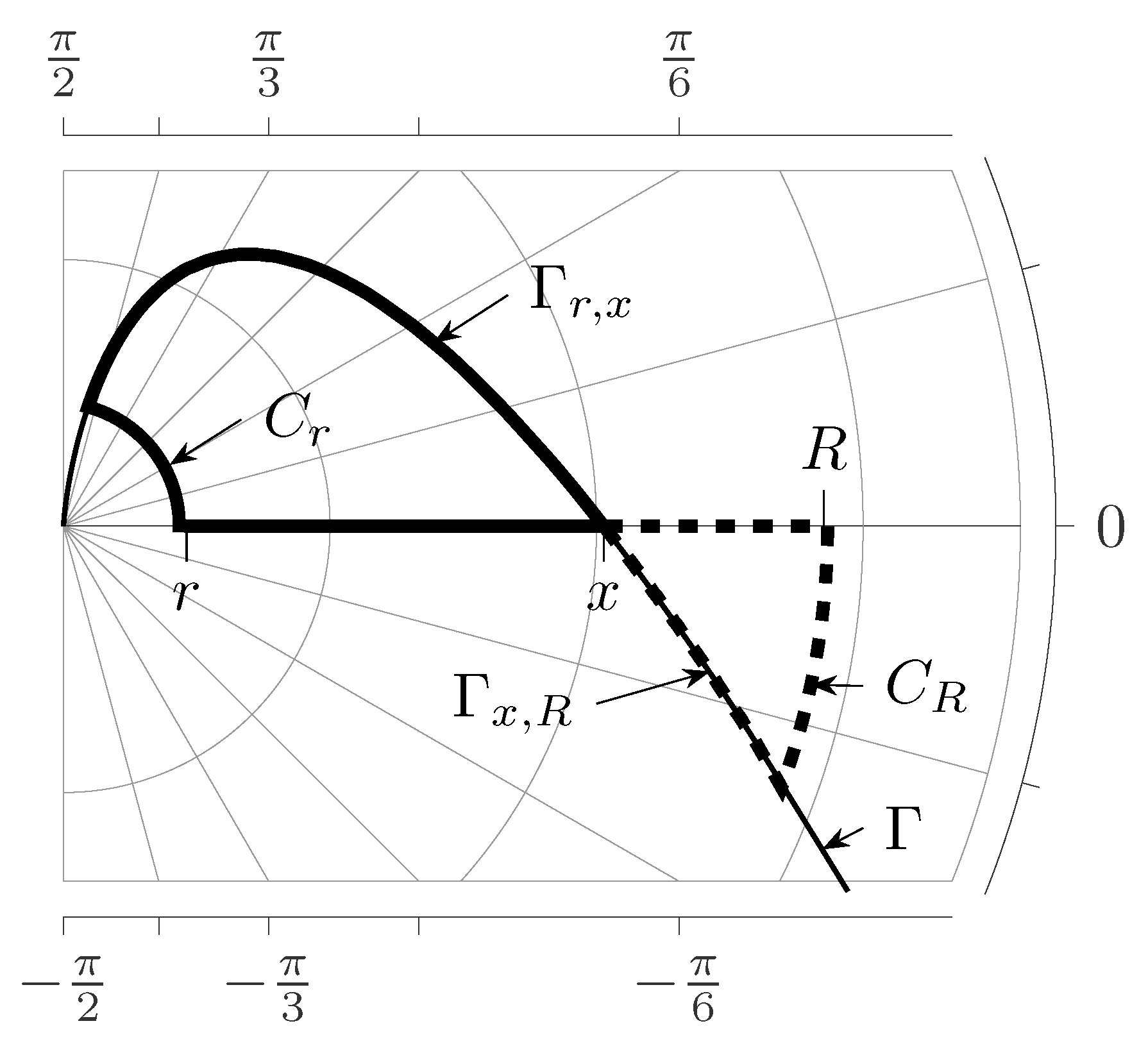
- Every contour starts in the point .
- 2.
- None of the contours Γ intersects the lines of the cut.
- 3.
- Moving from the point along the contour Γ we let it tend to infinity but in such a way that starting from some place all points have values of arguments within the limits:
- 1.
- if , then
- 2.
- if , thenwhere .
3. Main Results
- 1.
- If and for any valueswhere and
- 2.
- If , then for any and
- 3.
- If , then for any and any values x
- 1.
- 2.
- If , then for any and any x
- 3.
- If , then for any admissible α and θ
4. The Calculation of the Density and Distribution Function of a Stable Law
5. Conclusions
Funding
Acknowledgments
Conflicts of Interest
References
- Kotulski, M. Asymptotic distributions of continuous-time random walks: A probabilistic approach. J. Stat. Phys. 1995, 81, 777–792. [Google Scholar] [CrossRef]
- Kolokoltsov, V.N.; Korolev, V.Y.; Uchaikin, V.V. Fractional Stable Distributions. J. Math. Sci. 2001, 105, 2569–2576. [Google Scholar] [CrossRef]
- Montroll, E.W.; Weiss, G.H. Random Walks on Lattices. II. J. Math. Phys. 1965, 6, 167. [Google Scholar] [CrossRef]
- Scher, H.; Lax, M. Stochastic transport in a disordered solid. I. Theory. Phys. Rev. B 1973, 7, 4491–4502. [Google Scholar] [CrossRef]
- Scher, H.; Lax, M. Stochastic transport in a disordered solid. II. Impurity conduction. Phys. Rev. B 1973, 7, 4502–4519. [Google Scholar] [CrossRef]
- Klafter, J.; Blumen, A.; Shlesinger, M.F. Stochastic pathway to anomalous diffusion. Phys. Rev. A 1987, 35, 3081–3085. [Google Scholar] [CrossRef]
- Metzler, R.; Klafter, J. The random walk’s guide to anomalous diffusion: A fractional dynamics approach. Phys. Rep. 2000, 339, 1–77. [Google Scholar] [CrossRef]
- Zaburdaev, V.Y.; Denisov, S.I.; Klafter, J. Lévy walks. Rev. Mod. Phys. 2015, 87, 483–530. [Google Scholar] [CrossRef]
- Uchaikin, V.V. Montroll-Weiss problem, fractional equations, and stable distributions. Int. J. Theor. Phys. 2000, 39, 2087–2105. [Google Scholar] [CrossRef]
- Saenko, V.V. New Approach to Statistical Description of Fluctuating Particle Fluxes. Plasma Phys. Rep. 2009, 35, 1–13. [Google Scholar] [CrossRef]
- Saenko, V.V. Self-similarity of fluctuation particle fluxes in the plasma edge of the stellarator L-2M. Contrib. Plasma Phys. 2010, 50, 246–251. [Google Scholar] [CrossRef]
- Saenko, V.; Saenko, Y. Approximation of Microarray Gene Expression Profiles by the Stable Laws. Int. J. Environ. Eng. 2015, 2, 98–102. [Google Scholar]
- Saenko, V.; Saenko, Y. Application of the fractional stable distributions for approximation of gene expression profiles. Stat. Appl. Genet. Mol. Biol. 2015, 14, 295–306. [Google Scholar] [CrossRef] [PubMed][Green Version]
- Saenko, V.V. Fractional-Stable Statistics of the Genes Expression in the Next Generation Sequence Results. Math. Biol. Bioinform. 2016, 11, 278–287. [Google Scholar] [CrossRef]
- Ueda, H.R.; Hayashi, S.; Matsuyama, S.; Yomo, T.; Hashimoto, S.; Kay, S.A.; Hogenesch, J.B.; Iino, M. Universality and flexibility in gene expression from bacteria to human. Proc. Natl. Acad. Sci. USA 2004, 101, 3765–3769. [Google Scholar] [CrossRef]
- Hoyle, D.C.; Rattray, M.; Jupp, R.; Brass, A. Making sense of microarray data distributions. Bioinformatics 2002, 18, 576–584. [Google Scholar] [CrossRef]
- Furusawa, C.; Kaneko, K. Zipf’s Law in Gene Expression. Phys. Rev. Lett. 2003, 90, 8–11. [Google Scholar] [CrossRef]
- Saenko, V.V. Estimation of the Parameters of Fractional-Stable Laws by the Method of Minimum Distance. J. Math. Sci. 2016, 214, 101–114. [Google Scholar] [CrossRef]
- Schneider, W.R. Stable distributions: Fox function representation and generalization. In Stochastic Processes in Classical and Quantum Systems; Albeverio, S., Casati, G., Merlini, D., Eds.; Springer: Berlin/Heidelberg, Germany, 1986; Volume 262, pp. 497–511. [Google Scholar] [CrossRef]
- Schneider, W.R. Generalized one-sided stable distributions. In Stochastic Processes—Mathematics and Physics II. Lecture Notes in Mathematics; Albeverio, S., Blanchard, P., Streit, L., Eds.; Springer: Berlin/Heidelberg, Germany, 1987; Volume 1250, pp. 269–287. [Google Scholar] [CrossRef]
- Hoffmann–Jørgensen, J. Stable Densities. Theory Probab. Appl. 1994, 38, 350–355. [Google Scholar] [CrossRef]
- Zolotarev, V.M. On Representation of Densities of Stable Laws by Special Functions. Theory Probab. Appl. 1995, 39, 354–362. [Google Scholar] [CrossRef]
- Hatzinikitas, A.; Pachos, J.K. One-dimensional stable probability density functions for rational index 0<alpha<=2. Ann. Phys. 2008, 323, 3000–3019. [Google Scholar] [CrossRef]
- Penson, K.A.; Górska, K. Exact and Explicit Probability Densities for One-Sided Lévy Stable Distributions. Phys. Rev. Lett. 2010, 105, 210604. [Google Scholar] [CrossRef]
- Górska, K.; Penson, K.A. Lévy stable two-sided distributions: Exact and explicit densities for asymmetric case. Phys. Rev. E 2011, 83, 061125. [Google Scholar] [CrossRef] [PubMed]
- Pogány, T.K.; Nadarajah, S. Remarks on the Stable S α (β,γ,μ) Distribution. Methodol. Comput. Appl. Probab. 2015, 17, 515–524. [Google Scholar] [CrossRef]
- Mittnik, S.; Doganoglu, T.; Chenyao, D. Computing the probability density function of the stable Paretian distribution. Math. Comput. Model. 1999, 29, 235–240. [Google Scholar] [CrossRef]
- Menn, C.; Rachev, S.T. Calibrated FFT-based density approximations for α-stable distributions. Comput. Stat. Data Anal. 2006, 50, 1891–1904. [Google Scholar] [CrossRef]
- Nolan, J. An algorithm for evaluating stable densities in Zolotarev’s (M) parameterization. Math. Comput. Model. 1999, 29, 229–233. [Google Scholar] [CrossRef]
- Ament, S.; O’Neil, M. Accurate and efficient numerical calculation of stable densities via optimized quadrature and asymptotics. Stat. Comput. 2018, 28, 171–185. [Google Scholar] [CrossRef]
- Zolotarev, V.M. On the representation of stable laws by integrals. Sel. Transl. Math. Stat. Probab. 1964, 4, 84–88. [Google Scholar]
- Zolotarev, V.M. One-Dimensional Stable Distributions; American Mathematical Society: Providence, RI, USA, 1986. [Google Scholar]
- Nolan, J.P. Numerical calculation of stable densities and distribution functions. Commun. Stat. Stoch. Models 1997, 13, 759–774. [Google Scholar] [CrossRef]
- Arias-Calluari, K.; Alonso-Marroquin, F.; Harré, M.S. Closed-form solutions for the Lévy-stable distribution. Phys. Rev. E 2018, 98, 012103. [Google Scholar] [CrossRef] [PubMed]
- Bergström, H. On some expansions of stable distribution functions. Ark. Mat. 1952, 2, 375–378. [Google Scholar] [CrossRef]
- Uchaikin, V.V.; Zolotarev, V.M. Chance and Stability Stable Distributions and Their Applications; VSP: Utrecht, The Netherlands, 1999; p. 569. [Google Scholar]
- Nolan, J.P. Parameterizations and modes of stable distributions. Stat. Probab. Lett. 1998, 38, 187–195. [Google Scholar] [CrossRef]
- Royuela-del Val, J.; Simmross-Wattenberg, F.; Alberola-López, C. Libstable: Fast, parallel, and high-precision computation of α-stable distributions in R, C/C++, and MATLAB. J. Stat. Softw. 2017, 78. [Google Scholar] [CrossRef]
- Liang, Y.; Chen, W. A survey on computing Lévy stable distributions and a new MATLAB toolbox. Signal Process. 2013, 93, 242–251. [Google Scholar] [CrossRef]
- Veillette, M. MATLAB Code: Alpha-Stable Distributions. 2008. Available online: http://math.bu.edu/people/mveillet/research.html (accessed on 11 May 2020).
- Rimmer, R.H.; Nolan, J.P. Stable Distributions in Mathematica. Math. J. 2005, 9, 776–789. [Google Scholar]
- Nolan, J.P. John Nolan’s Stable Distribution Page. Available online: http://fs2.american.edu/jpnolan/www/stable/stable.html (accessed on 11 May 2020).
- Matsui, M.; Takemura, A. Some improvements in numerical evaluation of symmetric stable density and its derivatives. Commun. Stat. Theory Methods 2006, 35, 149–172. [Google Scholar] [CrossRef]
- Bening, V.E.; Korolev, V.Y.; Sukhorukova, T.A.; Gusarov, G.G.; Saenko, V.V.; Uchaikin, V.V.; Kolokoltsov, V.N. Fractionally stable distributions. In Stochastic Models of Structural Plasma Turbulence; Korolev, V.Y., Skvortsova, N.N., Eds.; Brill Academic Publishers: Utrecht, The Netherlands, 2006; pp. 175–244. [Google Scholar] [CrossRef]
- Bateman, H. Higher Transcendental Functions; McGraw-Hill Book Company, Inc.: New York, NY, USA, 1953; Volume 1, p. 302. [Google Scholar]
- GSL—GNU Scientific Library. Available online: http://www.gnu.org/software/gsl/ (accessed on 11 May 2020).


© 2020 by the author. Licensee MDPI, Basel, Switzerland. This article is an open access article distributed under the terms and conditions of the Creative Commons Attribution (CC BY) license (http://creativecommons.org/licenses/by/4.0/).
Share and Cite
Saenko, V. The Calculation of the Density and Distribution Functions of Strictly Stable Laws. Mathematics 2020, 8, 775. https://doi.org/10.3390/math8050775
Saenko V. The Calculation of the Density and Distribution Functions of Strictly Stable Laws. Mathematics. 2020; 8(5):775. https://doi.org/10.3390/math8050775
Chicago/Turabian StyleSaenko, Viacheslav. 2020. "The Calculation of the Density and Distribution Functions of Strictly Stable Laws" Mathematics 8, no. 5: 775. https://doi.org/10.3390/math8050775
APA StyleSaenko, V. (2020). The Calculation of the Density and Distribution Functions of Strictly Stable Laws. Mathematics, 8(5), 775. https://doi.org/10.3390/math8050775