Article

Volatility Timing: Pricing Barrier Options on DAX XETRA Index

1
School of Business and Communication, International University of La Rioja, 26006 Logroño, Spain
2
School of Economics and Business, University of Castilla-La Mancha, 02071 Albacete, Spain
3
Department of Economics and Finance, University of Castilla-La Mancha, 02071 Albacete, Spain
*
Author to whom correspondence should be addressed.
Mathematics 2020, 8(5), 722; https://doi.org/10.3390/math8050722
Submission received: 24 March 2020 / Revised: 29 April 2020 / Accepted: 2 May 2020 / Published: 4 May 2020

Abstract

:
This paper analyses the impact of different volatility structures on a range of traditional option pricing models for the valuation of call down and out style barrier options. The construction of a Risk-Neutral Probability Term Structure (RNPTS) is one of the main contributions of this research, which changes in parallel with regard to the Volatility Term Structure (VTS) in the main and traditional methods of option pricing. As a complementary study, we propose the valuation of options by assuming a constant or historical volatility. The study implements the GARCH (1,1) model with regard to the continuously compound returns of the DAX XETRA Index traded at daily frequency. Current methodology allows for obtaining accuracy forecasts of the realized market barrier option premiums. The paper highlights not only the importance of selecting the right model for option pricing, but also fitting the most accurate volatility structure.

1. Introduction

Instability in asset prices and periods of volatility or turbulence are two key elements that characterize and define the trend of financial markets. Thus, investors evaluate different opportunities, which can help to mitigate risks and maximize the expected return on their investments. One alternative that allows for reducing exposure to market risk and dealing with price turbulence is based on investment in hedging instruments and financial derivatives [1,2]. The derivatives market, and in particular financial options, allows the downside risk to be covered in the event of adverse movements in asset prices without constraining the investor of high performance in favorable market scenarios.
According to [3], a financial option is a contract that gives the holder the right, but not the obligation, to buy or sell an underlying at a price and for a period of time. These instruments represent a right for the buyer and an obligation for the issuer. We divide into call and put style options, depending on whether the right is to buy or to sell. Additionally, there are different types of options in regards to the time of exercise, such as European [4,5,6,7,8], American [9,10,11,12,13], Bermudian [14,15,16,17], and “path dependent” [18,19,20,21,22,23], among others. Within financial options, there are certain categories or exotic derivatives that are currently booming in the financial markets. Such is the case of barrier options, whose particularity can be seen in the activation or deactivation of its value when the price of the underlying (S0) reaches a certain barrier level (H). In this context, some authors, such as [24], develop new discrete dynamic models for the conditional valuation of barrier stock options assuming that their returns follow a normal inverse gaussian distribution (NIG). More recently, reference [25] studied the valuation of barrier options in contexts of uncertainty.
The aim of this paper is to verify via empirical analysis, which is the most accurate option pricing method with regard to knock-out barrier options: Binomial or Trinomial. We implement the aforementioned models under two underlying volatility assumptions. First, ex-ante historical volatility is estimated from past data and subsequent constant parameters of Binomial and Trinomial models are derived. Second, the construction of a daily dynamic volatility according to market fluctuations is considered to adapt the different parametrization of Binomial and Trinomial trees to a dynamic context. Specifically, we estimate GARCH (1,1) volatility by the maximum log-likelihood estimate (MLE) method for the case of a normal univariate distribution, thus fitting to the actual risk that is inherent in the financial market and, by extension, obtaining much more precise results. Moreover, the Black–Scholes model under historical volatility is implemented as a benchmark framework in our analysis.
In contrast to recent option pricing literature [26,27,28], one of the main contributions of this research is the construction of a Risk-Neutral Probability Term Structure (RNPTS), which changes in parallel with regard to the Volatility Term Structure (VTS). As a complementary study, we propose the valuation of options by assuming a constant or historical volatility. Both of the approaches refer us to divide the time period of analysis into two clearly defined intervals. The first timeframe corresponds to a parameter estimation period. This timeframe runs from February 2017 to February 2019 (in-sample period). The second time interval is focused on the forecasting (out-of-sample period) of conditional volatility models and, therefore, on pricing barrier options over the period that ranges from the end of February to the end of March 2019.
The reminder of the paper is structured in five sections. Section 2 reports the literature review. The first subsection in Section 3 describes the main model assumptions and properly details the option pricing methods from the characterization of the dynamic role of the volatility and the time-varying risk-neutral density; the second subsection depicts the considered data sample, where the main data sources and summary statistics are reported over the in-sample period. Options and underlying traded Index are extensively analyzed. Section 4 provides an out-of-sample forecasting analysis in which different option premiums are predicted and validated with regard to the realized market option price to avoid overfitting and spurious findings. Finally, Section 5 reports concluding remarks, providing significant evidence of less statistical error in those models fitted under dynamic volatility processes.

2. Literature Review

Throughout the extensive literature on financial derivatives and structured products, we can find numerous authors who propose different methods for option pricing. These models were originally based on the pricing of European options that do not pay dividends. However, with the increasing complexity of financial markets, extensions of these models emerge and may be applicable to the pricing of various exotic products, such as barrier options. We distinguish between models that are based on discrete-time numerical calculus, such as the Binomial tree and the Trinomial tree. The Binomial pricing approach, as proposed in the seminal paper of [29], assumes that the price of the underlying asset at the end of each period increases or decreases as a function of upward and downward multiplicative shocks. As a complement to the previous approach, the Trinomial pricing method that was developed by [30] and subsequently parametrized by [31] fits the underlying and option tree processes by a multiplicative neutral shock and an intermediate risk-neutral probability. Ref [32] propose an improvement of the Trinomial tree, the Adaptive mesh model, which introduces a tree with a small time step, ∆t, into another tree with a large ∆t. Authors, such as [33], state that the Trinomial model can be expressed as a reformulation of the Binomial process. More recently, the Trinomial tree valuation models, together with regime-switching techniques, emerge in the option pricing context [34,35,36,37,38,39,40].
Regarding continuous time models, the seminal study of [41] develop an analytical formula for the valuation of European-style options on assets that do not provide any known income, through the derivation of the heat equation. This model details the possibility of reaching a risk-free position by combining a long position in stocks with a short one in European call options (see Appendix B for further details). Otherwise, the Monte Carlo simulation emerges as a pillar in option pricing [42], which is based on the simulation of random variables to forecast the different trajectories of the underlying. Years later, a wide range of authors, both in the financial and computational literature, compare the accuracy of different Monte Carlo and quasi Monte Carlo techniques for derivative pricing, e.g., [43,44,45,46,47].
The pricing of the various derivative products that are based on traditional models requires information on the wide range of variables that affect the evolution of the underlying until maturity of the product. In particular, two of the most important are the expected return and the volatility of the underlying. A great deal of controversy has arisen in recent years over the choice of these input parameters since option premiums are extremely sensitive to both. The traditional mean-variance approach of [48] and subsequent theories show numerous statistical errors mainly arising from the choice of input parameters. On the one hand, references [49,50] show that historical returns are considered to be poor predictors of future returns. Recent studies have tried to change the usual approach by fitting the input parameters and reducing the statistical uncertainty of the model (see [51,52,53,54]). On the other hand, within the financial literature it is commonly accepted that most time series are generated by a random walk process, i.e., they are not stationary. Nevertheless, by conducting fist log-differences on the original data series (continuous compound returns), they usually show evidence of stationarity, but exhibit wide variations or volatility clusters, which indicates conditional heteroscedasticity in stock markets [55,56,57,58,59,60]. Thereby, reference [61] developed the model of Autoregressive Conditional Heteroscedasticity (ARCH) in order to capture the variability of financial time series from an autoregressive structure. Since its discovery in 1982, the development of autoregressive models has become a growing area, with all kinds of variations of the original scheme (e.g., [62,63,64,65]). The Generalized Autoregressive Conditional Heterocedasticity (GARCH) model proposed by [66] is one of the most popular.
Uncertainty plays a highly significant role in financial derivatives pricing. Thus, we find a wide range of approaches to estimate volatility along the different valuation methods proposed in the literature. Authors, such as [41], implement estimates of historical volatility of the underlying, while others, such as [67], implement stochastic volatility in option premium valuation models. With the advent of GARCH models to dynamically fit the volatility of the underlying assets, it was to be expected that such conditional estimates would be used in option valuation and hedging strategies [68]. Thus, reference [69] derive the option pricing model with GARCH-type volatility. Subsequent studies analyze the effect of this type of volatility on option pricing. Other authors, such as [70,71], find that the valuations obtained for short-term stock options under GARCH volatility processes more accurately reflect the realized option premiums traded in the market for such instruments with regard to the option premiums that were obtained via traditional models and historical volatility.
The latter studies start from the idea that the GARCH process for modelling variance is not independent and, therefore, this influences the modelling of the underlying price process. However, as an experimental study, in the current research, we assume that the opposite is also valid, i.e., that volatility and price of the underlying asset can be modeled as separate diffusion processes. In a nutshell, our paper differs from the previous ones in the fact that the methodology implemented is still not supported by a related theory.

3. Materials and Methods

3.1. Methodology

This subsection is divided into two clearly defined parts: option pricing methods and models for estimating and forecasting heteroscedasticity. While the former are focused on the different numerical calculus and analytical specifications proposed in the financial literature of option pricing, the latter show how the volatility input, which is required to make the mentioned relevant valuations, is properly estimated and predicted.

3.1.1. Option Pricing Models

In this subsection, we propose a wide spectral of models to shed some light on the choice of the right method for pricing knock-out call barrier options. Specifically, we focus on pricing down and out barrier options, Cdo, via two alternative discrete numerical calculus pricing methods: Binomial and Trinomial. Additionally, two different sources of uncertainty are considered when conducting the mentioned pricing methods: historical and GARCH (1,1) volatility. Calculus concerned to both the estimation of historical volatility and the forecast of a VTS are reported at Appendix A. We calibrate and implement this model for future forecasting by means of the Maximum Log-likelihood Estimation (MLE) method-. Moreover, the Black–Scholes under historical volatility is computed as a reference benchmark in option pricing.
Barrier options are a type of exotic financial derivatives, wherein the activation or deactivation of the option occurs when the price of the underlying asset reaches a certain level, called the barrier (H). They are always cheaper than similar options without a barrier (plain vanilla). Generally, they can be classified into knock-in barrier options and knock-out barrier options. Knock-in barrier options come into existence when the price of the underlying reaches the level of the barrier. In turn, they are classified into up and in barrier options (Cui), where the price of the underlying begins below the barrier level (H), with the option being triggered when the price increases and reaches the H level; and, down and in barrier options (Cdi). In these options, unlike the previous ones, the price of the underlying asset is above the barrier (H), thus being activated when the price decreases the H level. Moreover, knock-out barrier options are characterized by the fact that they cease to exist when the price of the underlying reaches the barrier. These options are classified as up and out (Cuo) options, i.e., those in which the price of the underlying begins below the barrier level (H), becoming null and void when the price rises and reaches the barrier. In down and out options (Cdo), unlike the previous ones, the price of the underlying asset starts above the barrier (H) and it is when the price decreases and reaches the barrier that it becomes null. Note that the latter are the ones assessed and priced on this research. In this regard, throughout this subsection, we describe their main valuation methods discussed above.
Within the numerical calculus methods, we distinguish two models that are based on discrete time, Binomial and Trinomial trees. First, we adapt the Binominal tree model, as proposed by [29] and recently conducted by [72,73], to conduct the price of the knock-out call option with n time steps until the expiration date as:
C d o , t Δ t = e r Δ t ( P u C d o , t u + P d C d o , t d ) .   ( S t Δ t > K )
where ( S t Δ t > K ) is a logical vector consisting in zeros and ones. This vector sets the option value in final nodes on or below the barrier level to zero. In addition, “ . ” defines a pointwise vector multiplication. C d o refers to the European call barrier premium, S t Δ t is the underlying price at time t Δ t , K is the strike price, and r is the risk-free rate.
Subsequently, the value of the knock-out call option is defined as a recursively backward procedure in time for j = n 1 ,   n 2 , , 0 , where the following vectors need to be defined for the underlying trajectories, S t :
S t = ( S t ( j , j ) S t ( j , j 2 ) S t ( j , j + 2 ) S t ( j , j ) ) = ( S 0 u j d 0 S 0 u j 2 d 2 S 0 u 2 d j 2 S 0 u 0 d j )
and the corresponding down and out option premium, C d o , t :
C d o , t = ( C d o , t ( j , j ) C d o , t ( j , j 2 ) C d o , t ( j , j + 2 ) C d o , t ( j , j ) ) = ( S t K ) + . ( S t > K )
Thus, for every t 0 , we separate into two different vectors regarding the option premium:
C d o , t u = ( C d o , t ( j , j ) C d o , t ( j , j 2 ) C d o , t ( j , j + 2 ) ) , C d o , t d = ( C d o , t ( j , j 2 ) C d o , t ( j , j + 2 ) C d o , t ( j , j ) )
Accordingly, the forward underlying trajectories at each t Δ t time can be expressed as:
S t Δ t = d ( S t ( j , j ) S t ( j , j 2 ) S t ( j , j + 2 ) ) = u ( S t ( j , j 2 ) S t ( j , j + 2 ) S t ( j , j ) )
Various parameters relating to the risk-neutral measures need to be estimated in order to conduct the prior forward simulation of trajectories for the underlying and the subsequent backward valuation of the option premium, as follows:
u = e σ Δ t d = 1 u = e σ Δ t P u = e r Δ t d u d P d = 1 P u
where u and d show the upward and downward multiplicative shocks experienced by the underlying asset. Pu is understood as the upward risk-neutral probability, Pd as the downward probability, and r is the risk-free interest rate. We consider that risk-neutral probabilities and multiplicative shocks are defined differently, depending on whether we introduce historical ( σ ) or GARCH volatility ( σ t ), obtaining fixed parameters with regard to the former ( u , d , P u , P d ) and time-varying vectors for the latter ( u t , d t , P u , t , P d , t ).
Second, an alternative discrete time specification for derivative pricing is the Trinomial tree pricing model [30], which states that the option premium depends on a broader branch of risk-neutral probabilities, Pu, Pm, and Pd (the probabilities of increase, neutrality, and decrease in each of the nodes, respectively). In the same vein as the Binomial model, n shows the time to maturity and ∆t is the length of the time step [3]. Unlike the Binomial model, the Trinomial trees display three possible movements of the price of the underlying asset in each node: up (u) if the price increases; middle (m), when the price remains stable; and, down (d) if the price decreases, where d = 1/u. As in the Binomial model, we follow the same backward process described in Equations (1)–(5) for the calculation of option premiums, just by adding a probability that the underlying remains constant. For simplicity, we do not show the matrix calculation any further.
Regarding the new risk-neutral parametrization, we can always choose u, so that the nodes rest on the barrier. The condition that u must meet is the following:
H = S 0 u N
or
ln H = ln S 0 + N ln   u
For N positive or negative, where:
ln u = ln H ln S 0 N
and
N = i n t [ ln H ln S 0 σ 3 Δ t + 0 , 5 ]
with i n t ( x ) being the integral part of x.
Additionally, the risk-neutral probabilities Pu, Pm, and Pd in the upper, middle, and lower branches of the Trinomial tree are chosen to coincide with the first two moments of the distribution of the underlying’s returns, so that
P u = ( r q σ 2 / 2 ) Δ t 2 ln u + σ 2 Δ t 2 ( ln u ) 2 P m = 1 σ 2 Δ t ( ln u ) 2 P d = ( r q σ 2 / 2 ) Δ t 2 ln u + σ 2 Δ t 2 ( ln u ) 2
where Pu, Pm, and Pd are the probabilities of the upper, middle, and lower branches. In the same vein as the Binomial model, in the Trinomial tree, we consider that risk-neutral probabilities and multiplicative shocks are defined differently, depending on whether we introduce historical ( σ ) or GARCH volatility ( σ t ), obtaining fixed parameters with regard to the former ( u , d , P u , P m , P d ) and time-varying vectors for the latter ( u t , d t , P u , t , P m , t , P d , t ).
Third, reference [41] report on the theory of option pricing, which shows how to hedge the short position of an option, by assuming the criterion of risk-free hedging, in order to derive the value of the partial hedge from the differential equation for the price of a European call option. Subsequent studies adapt the traditional Black–Scholes equation to the barrier derivative pricing. This valuation assumes that the probability distribution for the asset price at a future point in time is lognormal. An important question about barrier options is the frequency with which the asset price, S, is observed for determining whether the barrier has been reached. Equation (14) assumes that S is continuously observed. In addition, an increase in volatility might cause the price of the barrier option to fall.
The valuation of down and out barrier options via the analytical Black–Scholes method is characterized as:
C d o = S 0 N ( X 1 ) e q + T K e r T N ( X 1 σ T ) S 0 e q T ( H S 0 ) 2 λ N ( Y 1 ) + K e r T ( H S 0 ) 2 λ 2 N ( Y 1 σ T )
where q refers to the dividend yield (assumed as 0, since we are pricing European options without associated known income rates) and the rest of the parameters are defined, as follows:
λ = r q + σ 2 2 σ 2 X 1 = ln ( S 0 / H ) σ T + λ σ T Y 1 = ln ( H / S 0 ) σ T + λ σ T
The function N(x) is the cumulative probability that a variable with a standard normal distribution, N (0,1), is smaller than x. The rest of the variables must be known. C d o refers to the European call barrier option premium, S0 is the quoted price in t = 0, K is the strike price, r is the risk-free rate, σ is the volatility, and T is the time interval until the expiration date of the option.

3.1.2. Heteroscedasticity Methods
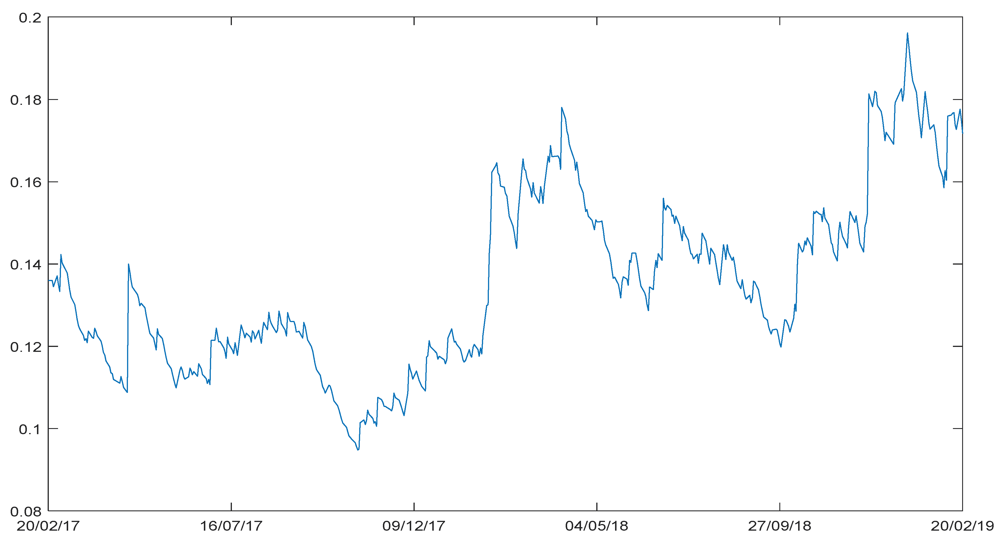
Historical volatility estimates current and future volatility by considering past events. It is considered as a benchmark in many volatility studies [57,74]. Statistically, it can be estimated as the square root of all observed returns up to the valuation date. As a starting point, we calculate the daily continuous returns from the closing prices of the underlying on each trading day ( r t = ln ( S t / S t 1 ) ). Subsequently, we compute the standard deviation of that series, s . Assuming that common year have 252 working days of market trading and based on the additive properties of continuous returns, the estimate of daily historical volatility in annualized terms can be expressed as σ = s 252 . In contrast to constant historical volatility, one of the most popular autoregressive conditional volatility models is the GARCH (p,q) specification, as proposed by [66]. Seminal studies in econometrics reveal that the simple GARCH (1,1) provide better results than more complex extensions of these specifications for different purposes and data samples [75,76,77]. This model states that the current conditional variance depends not only on squared innovations of the previous period (as in ARCH (1)), but also on its prior conditional variance. Thus, we fit the GARCH (1,1) model, as:
σ t 2 = ω + α ε t 1 2 + β σ t 1 2 ε t = σ t η t η t N ( 0 ,   1 )
where ω is the constant of the model and is closely related to the long-term variance of the process, α is the parameter of the ARCH component, β the parameter of the GARCH component model reflecting the persistence in volatility, ε t 1 are the innovations at time t 1 , and σ t 1 2 is the prior variance. η t are the standardized innovations of the process.
We fit this model via the MLE estimator. We include the following constraints to ensure the convergence of the MLE when estimating the GARCH model:
ω > 0 α 0 β 0 α + β < 1  
The latter constraint implies that the unconditional variance of process is finite, whereas its conditional variance evolves over time.
For regression purposes, in order to estimate the previous univariate GARCH (1,1) model, residuals of an AR(p) need to be fitted, by minimizing the sum of the squared errors:
r t = i = 1 p ϕ i r t i + ε t
where r t and r t i   denote both the current and the lagged asset’s returns and ε t are the residuals or innovations of current period. p denotes the maximum lag order and ϕ i is the parameter that measures persistence in the mean process.
Lastly, we forecast the future daily variance in n + 1 from the information available at the end of the day n 1 to construct the VTS:
E [ σ n + t 2 ] = V L + ( α + β ) t ( σ n 2 V L )
where E [ σ n + t 2 ] is the n + t daily forecast of the variance process and V L refers to the long term variance of the model, which indicates mean reversion.

3.2. Data

This subsection focuses on the analysis of the various barrier options and the underlying assets that are considered in this research. In particular, the frequency and the wide range of variables that directly and indirectly influence the option premiums are extensively analyzed in this section. First, Bolsas y Mercados Españoles (BME) freely provide all of the information regarding the five barrier options. These options are interpreted as down and out, since their premiums begin with value (the underlying, S0, begins trading above the barrier level) and decrease in value when its future price, St, falls below the stipulated level of the barrier, H. Note that, in all these options, the barrier level coincides with the strike price of the contracts, H = K. The selected barrier options have a time interval of n = 88 days from the issue date (20 February 2019) to maturity (21 June 2019). Documented data and other assessments can be extracted from Table 1.
Second, we consider two variables that are particularly relevant in the context of financial derivative valuation, the risk-free interest rate (r) and the time evolution of the underlying asset (St), in order to price the proposed financial options. Regarding the former, we consider the three-month EURIBOR traded on a daily basis as a proxy of the risk-free rate, r. The EURIBOR data is freely provided by the Quandl database for the period that spans from 17 February 2017 to 20 March 2019 (the risk-free interest rate is calculated as an annualized expectation of continuously compound daily returns estimated from zero-coupon bond prices for the period described above). With respect to the underlying asset, the daily historical prices of the DAX XETRA Index (underlying, St) from 17 February 2017 to 20 March 2019 have been extracted. The historical data relating to the price of the index are expressed in points. These data have been extracted from Yahoo finance via the ticker “^GDAXI” and they are particularly relevant for calculating the volatility of the proposed models.
From the top left subplot of Figure 1, we report on the prices of the DAX XETRA Index, which move as a random walk process with stochastic trend or unit root. Subsequently, when conducting first log-differences (top right subplot of Figure 1), we observe a stationary mean process. The autocorrelation functions and the Ljung-Box test [78] conducted from 1 to 20 lags barely show significant evidence of autocorrelation or persistence in the first moment of the distribution of continuous returns (mean) for the case of 4, 5, and 6 lags (significance at 10%). Additionally, the unit-root Augmented Dickey–Fuller test [79] suggests a significantly high evidence of stationarity for any of the analyzed lags. Regarding the variance equation, the series shows random variability, since logarithmic returns tend to form volatility clusters. This is confirmed by conducting autocorrelation functions and the Lagrange-Multiplier test on squared residuals. Thereby, the use of historical volatility as an estimator of market uncertainty underestimates actual market risk. Based on the above, in subsequent sections, we conduct a VTS, i.e., we express the volatility as a function of the time interval, rather than working with a constant volatility for all investment horizons. We forecast volatility based on the GARCH (1,1) model to generate this conditional risk structure on a daily basis.
Furthermore, from the kernel graph (bottom left of Figure 1), we report on the fact that DAX XETRA Index returns do not follow a normal distribution as the empirical distribution is more pointed than the Standard Gaussian, i.e., the returns of the DAX XETRA index follow a leptokurtic distribution. It implies that kurtosis is higher than normal (kurtosis = 4.5186 > 3). Additionally, we can analyze the non-normality of the DAX XETRA from the tail behavior that was observed in the qqplot (bottom right subplot of Figure 1). This plot compares the quantiles of the empirical distribution of the DAX XETRA returns (blue line) with respect to the quantiles of a standard normal distribution (red dotted line). In the same vein, we report on a substantial deviation of the empirical distribution from the normal quantiles, providing clear evidence of heavy tails and negative skewness (−0.1292).

4. Results and Discussion

This section reports on the main results and conclusions that can be extracted from the valuation of a wide range of knock-out barrier options, with regard to the very different numerical and analytical methods that re described in Section 3, concluding which of these is the most accurate when forecasting the option premium over the out-of-sample period. Additionally, a line graph reports on the trend of these models with regard to the option premium, thus shedding light on which is the method that most resembles the current state of the financial markets. Additionally, three measures of quantitative nature have been implemented to evaluate the predictive accuracy of the proposed pricing methods, as well as two different tests to assess the robustness of the out-of-sample analysis results (Matlab codes for option pricing are available in Supplementary Materials).

4.1. Conducting the Volatility. In-Sample and Out-of-Sample Analysis

A VTS has been conducted based on the GARCH type models, as a robust alternative to traditional historical volatility, to obtain a more reliable approximation to the option traded premiums and, therefore, to get a minimum error when forecasting. Two clearly differentiated processes are required to obtain this VTS: the first is based on the estimation of the parameters of the GARCH models and the second is an out-of-sample forecasting process of the future volatility structure.
First, we focus on the in-sample estimation of time-varying GARCH volatility. We fit the GARCH (1,1) model from the residuals of a prior autoregressive AR(4) estimation. These estimations are conducted on the basis of continuous compound returns of the DAX-XETRA Index for the interval between the end of February 2017 and the end of February 2019 (issue of the barrier options), obtaining a time-series of volatility that includes 508 daily frequency data and whose mere purpose is to calibrate the parameters of our GARCH model (ω, α, β) on that date [80]. We implement the Maximum Log-likelihood estimate (MLE) method for the case of a univariate normal distribution to conduct such estimation (see Appendix A).
From Table 2, we analyze the estimated parameters in three stages, mean equation, variance process, and information criteria. First, the estimated parameters reported in Panel A indicate weak persistence with respect to the mean equation. We observe that the autoregressive parameter, ϕ i , is only significant for the case of the 4th lag order, as suggested in prior analysis (Section 3.2). Second, when considering the variance equation (Panel B), we report on a less statistical significance of the parameters that are associated to the long-term variance, ω , and the squared innovations, α , whereas a very significant persistence in volatility, β , is observed. Third, from Panel C, we report on the values a wide range of information criteria previously conducted to select the most accurate autoregressive model with respect to the data sample. After an exhaustive analysis from a range of ARMA-GARCH models, the AR(4)-GARCH(1,1) is selected based on the lower AIC, BIC, SBT, and HQIC obtained by the model. Additionally, this model depicts the largest value of the log-likelihood. Additionally, the Ljung–Box ( Q ) and Lagrange multiplier ( L M ) statistics (Panel A and Panel B, respectively) reveal a large decrease in the presence of time dependence in residuals and squared residuals.
From Figure 2, we report on the evolution of volatility based on the estimate fitted by the AR(4)-GARCH(1,1) model. Based on this figure, volatility seems to exhibit a less turbulent and moderately smoothed trend until the end of 2017, whereas more fluctuations and remarkable peaks are described from early 2018 to the end of 2019. Specifically, these variations reach their peak at the end of 2018, which corresponds to the biggest Christmas Eve downturn in history of the Dow Jones Industrial Average Index, driven by the sell-off coming off the back of news reports that President Trump sought to fire FED Chair, following the FED’s policy to increase interest rates at the December meeting. The cited Index fell to a 2018 low 21,712 points before experiencing its largest single day profit ever on the next trading day on further information that Trump does not have that authority. This event, along with concerns regarding the impact of the trade war with China, undoubtedly caused widespread havoc and severe turmoil in the global financial markets. Thus, by fitting GARCH models, we can include these dynamics in the volatility trend that are usually underestimated or overestimated when just considering a constant volatility estimate, such as historical volatility.
Second, we implement the GARCH model to forecast volatility over the period than spans from the 21 February 2019 to the 21 June 2019 once the different parameters have been estimated on 20 February 2019, and taking them as a reference. From the top subplot of Figure 3, we report on a convergence to a stable long-term variance (0.0219), as the time interval increases. On the other hand, the bottom subplot of Figure 3 shows the VTS conducted based on the GARCH (1,1) model. The conditional structure has a negative slope and shows a smoothed trend over the time horizon, which allow for the different market movements to be reflected in the various considered option premiums (note that both graphs (Figure 3) show the daily evolution of variance and conditional volatility, both expressed in annualized terms multiplying by 252 and √252, respectively).
Third, in contrast to GARCH volatility, we just consider the in-sample period to compute historical volatility, since it is calculated based on past data. Thereby, we obtain the data referring to the period between February 2017 and February 2019. Historical volatility assumes that the risk during the entire time interval remains constant—historical volatility is a measure of the intensity of random variations that occur in assets’ returns over a given time horizon. We calculate the standard deviation (volatility) from the continuous compound returns once we have obtained the data on the DAX XETRA Index daily traded prices. We annualize daily volatility multiplying by √252, reaching an annual equivalent volatility of 0.1372 for the numerical calculus of the various barrier option pricing methods.

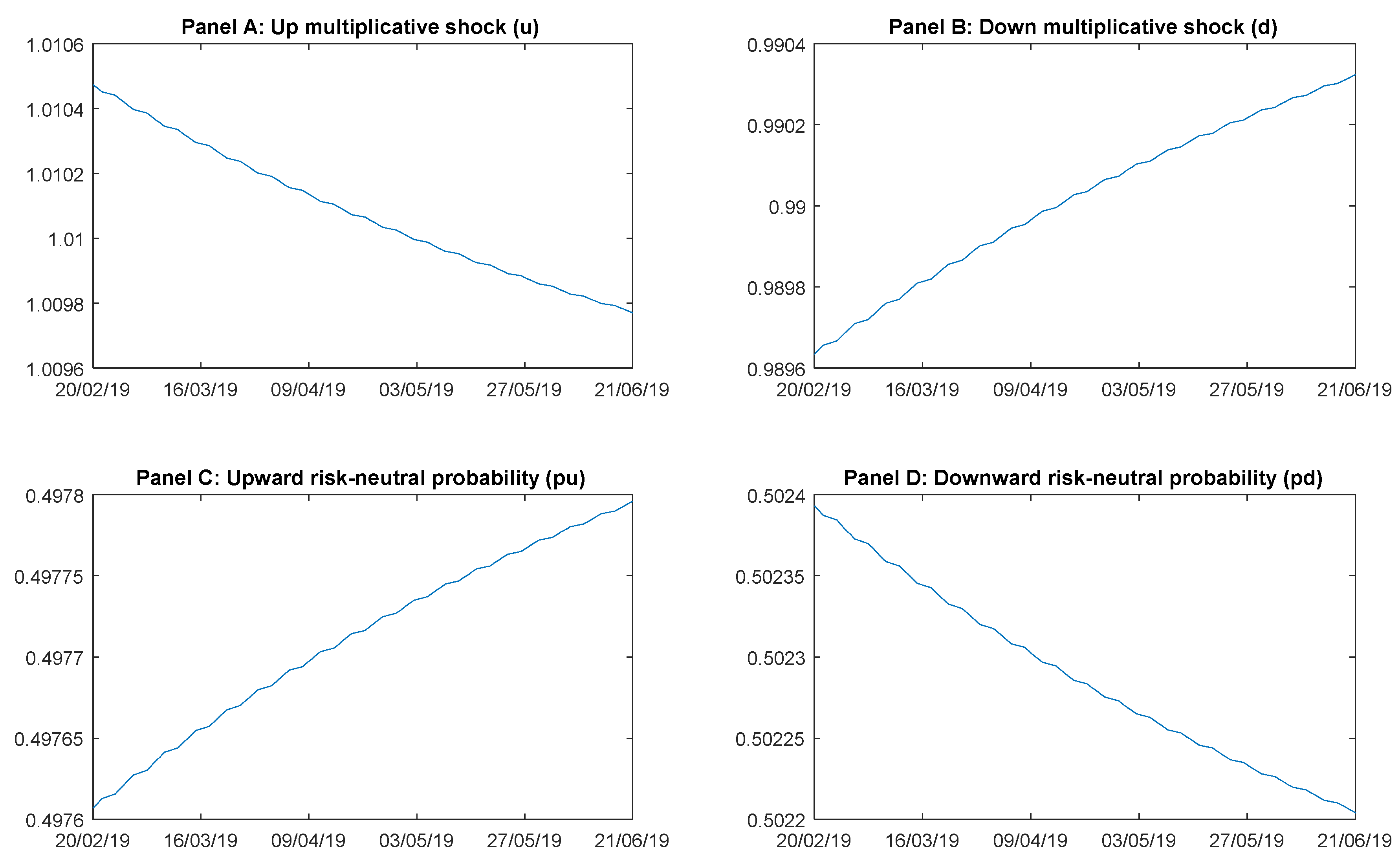
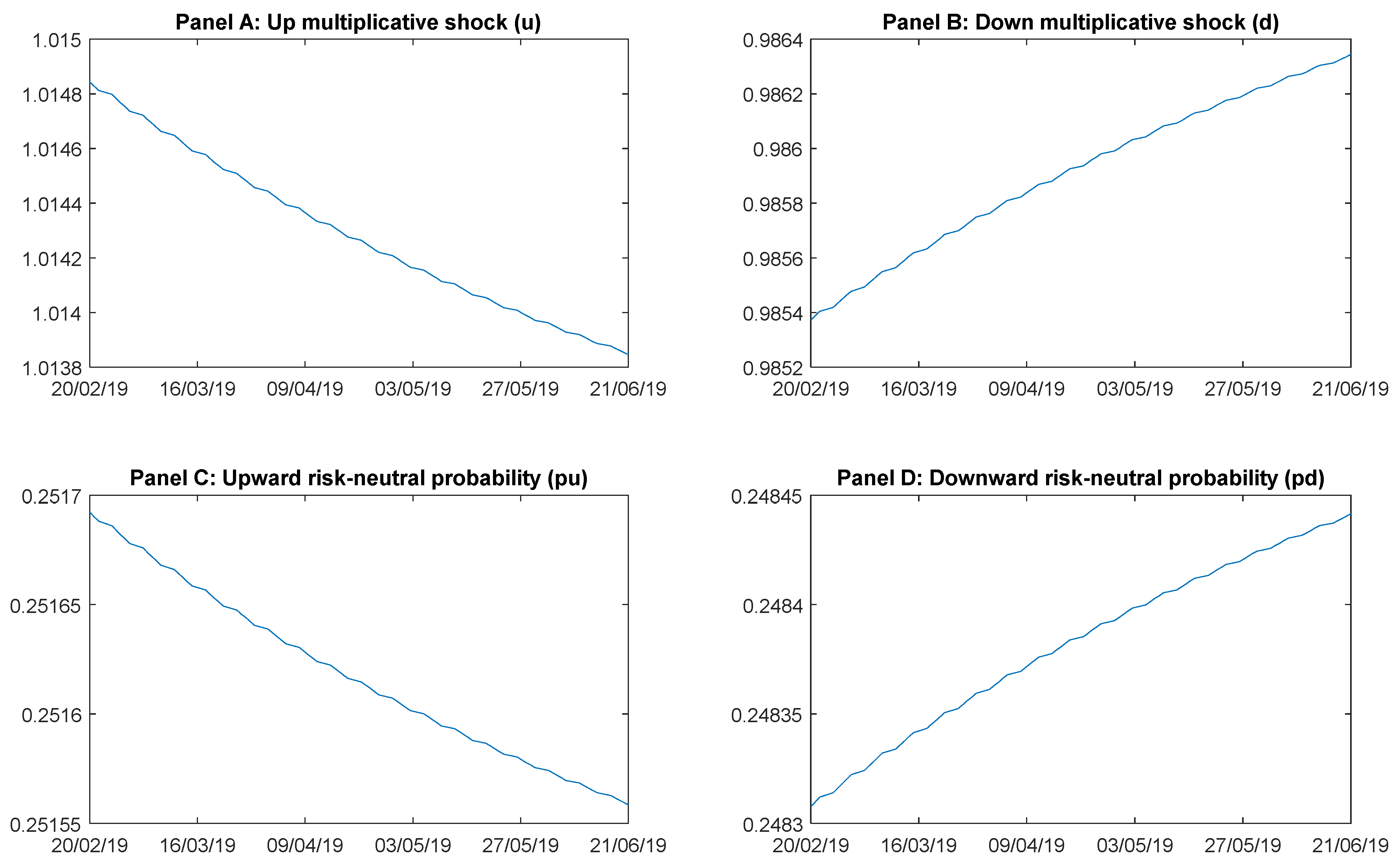
4.2. Out-of-Sample Risk Neutral Density Forecasting

Multiplicative shocks and risk neutral probabilities need to be computed prior to the implementation of the different discrete numerical time option pricing models (Binomial and Trinomial). These parameters refer to upward and downward movements for the case of the Binomial model, whereas they are classified into upward, neutral and downward movements for the case of the Trinomial tree model. Specifically, in this section, we compare the static parameters of the Binomial under historical volatility model with regard to the dynamic parameters obtained via the GARCH (1,1) Binomial method, to assess their effect on the different barrier option premiums. We follow the same procedure for the case of the Trinomial model, while comparing the risk neutral parameters fitted under historical and GARCH volatility. Note that, for simplicity, all reported risk-neutral parameters and plots refer to the H = 10,000 points. The parameters of the remaining models provide the same insight, with the exception of the H = 10,800 barrier option.
Based on the temporal evolution of the risk-neutral parameters (see Figure 4), we observe that in general the dynamic up multiplicative shock of the GARCH (1,1) Binomial method, u t , is higher than the fixed parameter obtained for the historical Binomial method ( u = 1.0084 ). Conversely, the dynamic down multiplicative shock of the GARCH (1,1) Binomial method, d t , is lower than that of the historical model ( d = 0.9916 ). It leads to a lower time-varying upward risk-neutral probability, P u , t , and a higher downward risk-neutral probability, P d , t , of the Binomial-GARCH (1,1) method with regard to those that are associated to the Binomial-Historical ( P u = 0.4982 , P d = 0.5018 ).
As for the risk-neutral parameters of the Trinomial model (see Figure 5), we observe that they follow an opposite evolution to that of the Binomial model. Thereby, the upward risk-neutral probability of the historical Trinomial method turns out to be lower ( P u = 0.2513 ) than that of the Trinomial GARCH (1,1) method, P u , t , leading to a higher downward risk-neutral probability ( P d = 0.2487 ). The above cause the forecasting of the barrier option premium price with H = 10.000 points is more similar to the market premium, i.e., a lower forecasting error is obtained. The above is mainly explained by the dynamics of the GARCH (1,1) model, which generates a daily VTS that allows for obtaining a better fit with the empirical variations in the uncertainty of financial markets. This opposite direction in the risk-neutral probabilities causes the Trinomial pricing under the GARCH (1,1) model to obtain a higher forecasting error than the remaining models based on constant historical volatility. The above is mainly explained by the dynamics of the GARCH (1,1) model, which generates a daily VTS that allows for obtaining a better fit with the empirical variations in the uncertainty of financial markets.

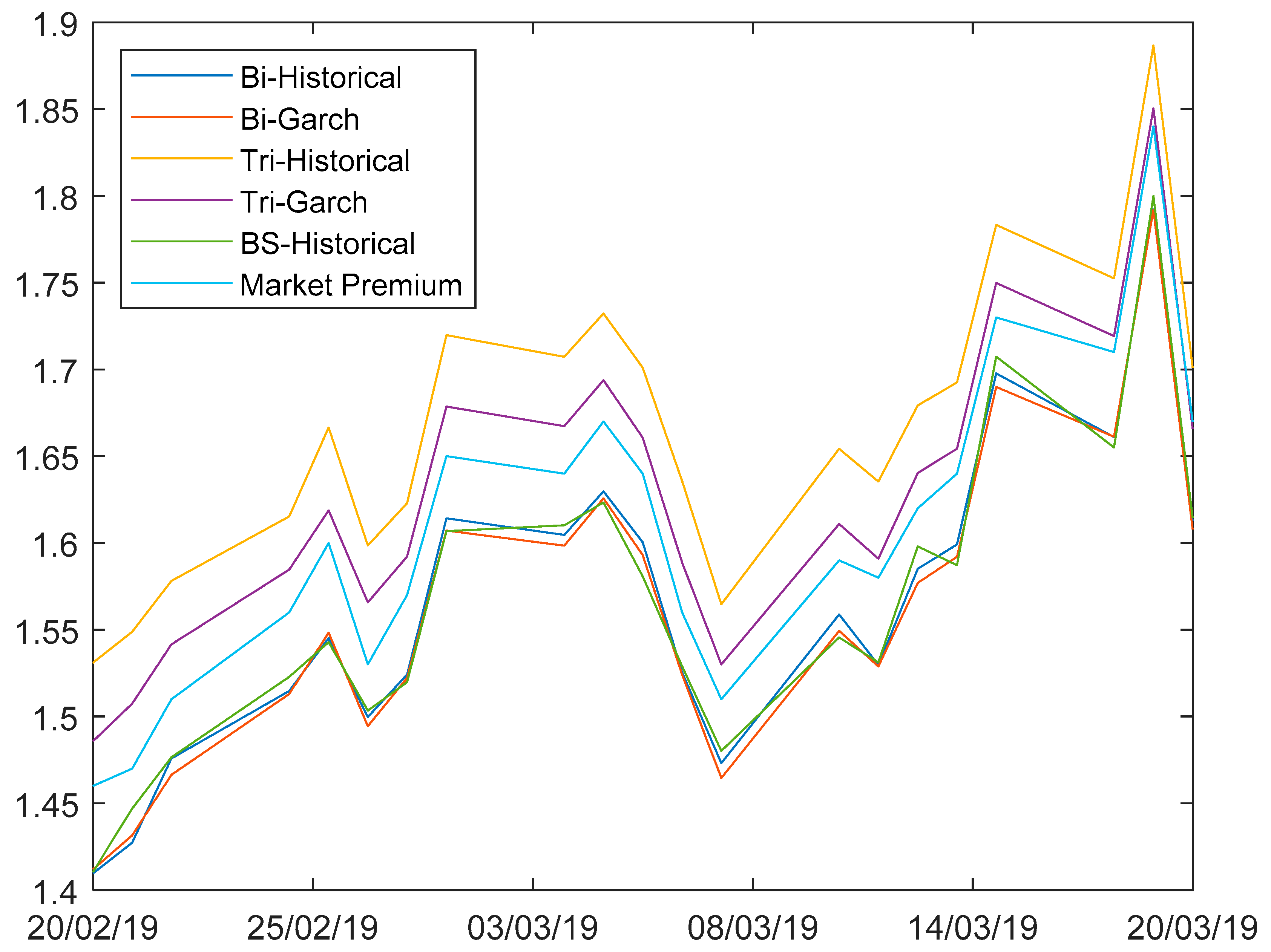
4.3. Robustness Check. Accuracy Forecasting Assessment for Option Premiums

This subsection aims to show a comparison of the diverse barrier option premiums priced by way of the wide variety of pricing methods that are discussed in Section 3. We determine which of these models is the most accurate in predictive terms when forecasting the premiums of down and out call barrier options. This subsection is organized in three stages. First, the particularities of the calculation and forecasting of the proposed pricing models are discussed. Second, a comparative graphic analysis of the different models is reported. Third, a robustness analysis is carried out in order to shed light on the validity of the models.
First, in contrast to recent literature [26,27,28], this research provides a new methodology for knock-out barrier option pricing by fitting the traditional discrete Binomial and Trinomial methods to a dynamic context. Specifically, time step size of the different trees, ∆t, is adapted to a daily VTS prior that is estimated from a GARCH (1,1) model. Thereby, we obtain what we call in this research the RNPTS, which changes in parallel with regard to the dynamic volatility of each tree step. Additionally, as a robustness test of our results, other methods have been proposed, such as the inclusion of historical volatility in the aforementioned Binomial and Trinomial trees or the option pricing by way of the Black–Scholes model, as previously described in Section 3 (we only provide the detailed explanation of Binomial and Trinomial methods, due to their greater complexity and arduous calculus process).
Binomial and Trinomial trees have been constructed on a daily step basis, ∆t = 1 day, for the time interval from 20 February (issue date) to 21 June 2019 (maturity date), obtaining 21 trees with respect to historical volatility and another 21 trees regarding GARCH (1,1) volatility, as reported in Figure 6. The first tree has a number of steps, n, of 88 days and the last reaches a total of n = 68 days (see Figure 6), i.e., we can forecast the price of the premiums, C ^ t , of the selected barrier options over 21 days (from 20 February to 20 March 2019).
Second, the option prices conducted on the basis of the above methods for the five selected barrier options (H = 10,000, H = 10,200, H = 10,400, H = 10,600, H = 10,800) are compared with regard to the prices of the realized market option premiums in order to clarify which valuation method reaches the least forecasting error. On the document, we only perform graphical analysis of the call barrier option with H = 10,000; for the remaining options (H = 10,200, H = 10,400, H = 10,600, H = 10,800), see Appendix D. Figure 7 compares the different prices reached for the H = 10,000 call barrier option. This line graph displays a dynamic comparative analysis, in which we report on the different paths followed by the barrier option premium prices computed via the various commented pricing methods. As can be extracted from the plot, all of the pricing methods follow a very similar trend to that of the realized market premium and there are no substantial differences between them. Even then, the most accurate pricing method is the Trinomial tree under GARCH volatility for most barriers, except for H = 10,800, which is mainly due to the calibration of a daily dynamic volatility instead of fitting a constant volatility for the whole period. Conversely, the Trinomial tree under historical volatility is the method that reports option prices far from the realized market premiums, which does not seem to be a suitable method in terms of forecasting the option premium.
Third, to validate our models and to test their robustness, we present three quantitative measures to assess the accuracy of a forecasting, as reported on Appendix C: the Mean Square Error (MSE), the Root Mean Square Error (RMSE), and the Mean Absolute Error (MAE). These methods are based on the assessment of the forecasting errors of each of the selected call barrier options with respect to their realized market prices (see Table 3). Additionally, two different statistical tests are implemented to check the validity of these quantitative tools: the Diebold and Mariano (1995) and the Harvey et al. (1997) tests, which report on whether the forecasting error of the prior most accurate model (Trinomial-GARCH) with regard to the mean error techniques, is significantly lower than that reached by the other pricing methods when forecasting the market premium of these options.
As reported on Table 3, in fact, the most accurate pricing method for computing the premium of the wide variety of selected knock-out barrier options on DAX XETRA Index is consistently the Trinomial tree under GARCH (1,1) volatility for almost all of the barrier pricing models. This result is due to the lower forecasting error with respect to the different methods of evaluating the accuracy of the forecasting models. Therefore, we observe that previous models are a robust alternative, as they provide minimal deviations from the market realized premium for each scenario. Additionally, Diebold and Mariano (DM) and the Harvey et al. (HLN) statistics confirm the previous results and provide greater robustness to the empirical analysis, as the forecasting errors are statistically significant with respect to those obtained through the application of the rest of the models. Note that most of them are statistically significant at 99%, since the p-values are less than 1% in all cases, except for the H = 10,600 points barrier option.

5. Conclusions and Remarks

Within the world of financial derivatives and, in particular, with regard to European-style barrier options, we observe a great heterogeneity in terms of the models dedicated to the pricing of this type of instrument. Thus, after the exhaustive analysis documented in this research, find from analytical models (Black–Scholes) to methods based on numerical calculation, such as the discrete time models (Binomial and Trinomial trees) and the continuous time processes (Monte Carlo simulation).
The analysis of persistence in the returns of financial assets is a very interesting line of research due to the controversy that exists regarding whether this phenomenon occurs and, if so, whether this persistence only exists in short periods of time or in longer time horizons. Specifically, persistence refers to the term autocorrelation or correlation of a variable with its more recent past. Furthermore, the existence of this phenomenon can be assessed for both the first moments of the probability distribution (mean) and the second moments (variance and deviation). The presence of autocorrelation in the second moments of the distribution of financial return processes is very common in time-series analysis. This means that estimates based on the assumption of constant or historical volatility are underestimating (positive autocorrelation) or overestimating (negative autocorrelation) the true risk inherent in financial markets. Therefore, the use of conditional volatility models, such as moving volatility windows, exponential smoothing models, or GARCH models, is one resource for resolving this difference in estimates. These models make it possible to adapt the volatility estimate to the time of valuation, eliminating the possible time biases caused by different financial market trends.
The interest of this paper is to gather traditional option pricing models and new trends in fitting and forecasting volatility to conduct the price of a wide range of European style barrier options with different strike prices and barrier levels. Thereby, in Section 3, we reported the entire theoretical framework necessary for the understanding of this type of exotic derivative products and their calculation via different methodologies. Specifically, in this section, we explain the general context of barrier options, emphasizing their main particularities in valuation. Subsequently, we provide an empirical analysis in Section 5 in order to display from a more realistic point of view how each one of these methods behaves. Furthermore, this research tries to find out which of the proposed methods is more accurate in terms of forecasting option premiums for various barrier options. It is a matter of clarifying which method reaches the least forecasting error in terms of predictive accuracy with respect to the realized market premium. Thus, three quantitative mean error methods are implemented in order to assess the accuracy of a forecasting, such as MSE, RMSE, and MAE. Additionally, we fit the DM and HLN statistics to provide significant evidence of the robustness of the obtained results.
We conclude that the Trinomial volatility-adjusted GARCH (1,1) method is the pricing method that best fits the realized market barrier option premiums, since it is the method that exhibits the least error in terms of forecasting accuracy. Complementarily, the differences of this model with respect to the others are confirmed as being highly statistically significant for most of the analyzed barrier options, based on the DM and HLN statistics. The above provides greater robustness to assessments of current research, inducing important implications mainly for investors and risk managers in investment strategies, thus helping to minimize the financial risks. In concrete, the use of the Trinomial volatility-adjusted GARCH method to price barrier options might allow for reaching the best forecast of the option premiums.
As far as the potential limitations of this research are concerned, the first one could be assume a normal distribution, which is commonly accepted in the financial literature. However, other sorts of non-normal distributions could have been assumed, which would take into account, for example, heavy tails, as t-student distribution, hyperbolic distributions, etc. In this way, returns of empirical estimates could be better adjusted. In addition, when fitting the empirical distribution, one could consider not only the dynamics in the second moment (conditional volatility), but also the third and fourth order time-varying moments, skewness, and kurtosis. Finally, we limit our analysis to European call barrier options.
Thus, future research could consist of applying this analysis on American (instead of European) barrier options, by studying, in depth, the particularities of this type of financial derivatives. Furthermore, this study could be broadened on barrier put (instead of call) options. In addition, we could assume alternative non-normal distributions and include the modelling of higher order moments when estimating the GARCH processes via MLE. Finally, it can be interesting to extend our analysis to stochastic risk-free rate models.

Supplementary Materials

The following are available online at https://www.mdpi.com/2227-7390/8/5/722/s1.

Author Contributions

Data curation, C.E. and E.I.; Formal analysis, C.E. and E.I.; Funding acquisition, F.J.; Investigation, C.E. and E.I.; Methodology, C.E.; Project administration, F.J.; Software, C.E.; Supervision, F.J.; Validation, E.I.; Writing—original draft, E.I.; Writing—review & editing, C.E. and F.J. All authors have read and agreed to the published version of the manuscript.

Funding

This research was funded by Spanish Ministerio de Economía, Industria y Competitividad, grant number ECO2017-89715-P.

Conflicts of Interest

The authors declare no conflict of interest.

Appendix A. Estimation by Maximum Log-Likelihood (MLE)

The parameters that are related to conditional volatility and VTS documented in this work have been estimated by conducting the MLE method. Specifically, a univariate GARCH model is used to fit the volatility of the DAX XETRA index. In this section, the steps for the estimation are analyzed. First, we consider that the standarized innovations of a prior AR (p) model follow a univariate normal distribution, η t N ( 0 ,   1 ) . Given this, its associated density function is as follows:
f ( x / ε t , σ t 2 ) = 1 2 π σ t 2   e ( ε t 2 2 σ t 2 )
Subsequently, the conditional likelihood function is obtained as a multiplier of the density function from 1 to n :
L ( ε t , σ t 2 / x i ) = t = 1 T 1 2 π σ t 2   e ( ε t 2 2 σ t 2 ) L ( ε t , σ t 2 / x i ) = 2 π n 2   σ 2 n 2   e ( 1 2 i = 1 n ε t 2 σ t 2 )
Maximizing the conditional likelihood function is equivalent to maixmizing its logarithm as ln(.) is a strictly increasing function. Due to its ease of handle, we express the cited estimator via logarithims as:
l o g L ( ε t , σ t 2 / x i ) = n 2 l o g ( 2 π σ t 2 ) 1 2 t = 1 T ε t 2 σ t 2
where σ t 2 = ω + α ε t 1 2 + β σ t 1 2 needs to be recursively evaluated.

Appendix B. Derivation of the Traditional Black–Scholes Equation for European Option Pricing

The stochastic process of the underlying asset (St) follows the geometric Brownian model:
d S t S t = μ   d t + σ Z t
where μ is the expected rate of return, σ is the volatility, and Z t is the standard Wiener process (Brownian model).
According to [81], we consider a portfolio Π that is composed of the purchase of Δ underlying asset and the short sale of a call option on that underlying asset. The value of the portfolio Π = ( S t , t ) at time t is:
= c + Δ t S t
where c = c ( S t , t ) denotes the value of the call at a time t, which expires at T ,   t T , on a share with a price S t .
As a final objective, Black and Scholes set out to obtain a risk-free portfolio Π. For this reason, reference [81] studied the variation of the portfolio, with this being a random variable:
d Π = Δ d S     d C
The value of the option c = c ( S t , t ) will be a function of time and the value of the action. As S t is a random variable, we will use the Itô’s lemma to obtain the stochastic differential equation:
d C = ( C S + μ S C S + 1 2   σ 2 S 2 2 C S 2 ) d t + ( σ S C S d Z )
To obtain the stochastic variation of the portfolio, we substitute the Equations (A18) and (A21) in the Equation (A20):
d Π = Δ S μ d t + Δ S σ d Z ( C S + μ S C S + 1 2   σ 2 S 2 2 C S 2 ) d t ( σ S C S d Z ) d t
One part of the above equation is deterministic and the other stochastic, so we proceed to group terms:
d Π = ( Δ μ S C S μ S C S 1 2   σ 2 S 2 2 C S 2 ) d t + ( Δ S σ σ S C S ) d Z .  
To ensure that this portfolio Π is risk-free, ( Δ S σ σ S C S ) = 0 , then
Δ = C S
Therefore, by replacing Equation (A23) in Equation (A24), the performance of our portfolio Π is:
d Π = ( C S t + 1 2   σ 2 S 2 2 C S 2 ) d t
Since the portfolio is no longer at risk, its return is equal to that of a risk-free bond:
d Π = Π r d t
We equate Equation (A11) with Equation (A12) by obtaining:
( C S t + 1 2   σ 2 S 2 2 C S 2 ) d t = Π r d t
The value of the portfolio is given by Equation (A5), so if we substitute:
( C S t + 1 2   σ 2 S 2 2 C S 2 ) = ( C S r S r C )
After all of this, we obtain the parabolic differential equation, called the Black–Scholes equation:
C t + 1 2   σ 2 S 2 2 C S 2 + r S C S r C = 0
As a complement to the formulation of the option pricing model, we must add and highlight an auxiliary condition, which tells us that the value of a European call at the time of expiration must be met:
C ( S ,   T ) = m a x ( S X ,   0 )
Lastly, the Black–Scholes-Merton formula for call european option pricing is:
C = S 0 N ( d 1 ) K e r T N ( d 2 )

Appendix C. Robustness Forecasting Accuracy Methods

We provide three different mean error quantitative tools to assess the accuracy of forecasting premiums in this appendix. Additionally, two different tests are reported to validate the aforementioned measures of error.
First, the MSE is proposed, which is calculated as the average square difference between the estimated values (market premium price) and what is estimated (premium price calculated by the different barrier option valuation methods).
M S E = 1 n t = 1 n ( C t C ^ t ) 2
where C t refers to the realized market premium price of the barrier option and, C ^ t , to the predicted premium price with each of the models.
Second, the RMSE is the residual standard deviation, i.e., how far the calculated barrier option premium is from the realized value of the barrier option for the same time interval.
R M S E = 1 n t = 1 n ( C t C ^ t ) 2 = M S E
Third, the MAE is calculated as the difference, in absolute value, between the realized premium value of the barrier option and that calculated through the four valuation methods that were used throughout the work.
M A E = 1 n t = 1 n | C t C ^ t |
On the other hand, reference [82] proposed the Diebold and Mariano (DM) test, whose aim was to compare two different forecasting experiments for the same variable in an environment of independence and to examine whether they were accurate. These authors considered a null hypothesis of no difference between the original data observed in the market and the forecasting s of the models to be used.
Being the errors of each forecasting model:
e 1 t = y ^ 1 , t y t e 2 t = y ^ 2 , t y t
where y ^ 1 , t and y ^ 2 , t refer to the actual values and, y t to the forecast data set.
Taking the errors as functions f ( e 1 t ) and f ( e 2 t ) , which refer to the associated losses at each of the moments t of the original data, we define the differential of the models, being compared as:
d t = f ( e 1 t ) f ( e 2 t )
If the forecasting s are the same, dt will be zero for all t. This is where the hypotheses proposed by [82] come in:
H 0 : E ( d t ) = 0   t   ( t h e   m o d e l s   a r e   i d e n t i c a l ) H 1 : E ( d t ) 0   t   ( t h e   m o d e l s   a r e   d i f f e r e n t )
Therefore, the test statistic developed by [81] is:
D M = d ¯ 2 π f d ^ ( 0 ) T
Ref. [83] propose a modification of the Diebold and Mariano test, whose main objective is based on working with small samples. The first modification uses an unbiased estimator of the dt variance while assuming that, for forecasting horizons, the differential loss dt has autocovariance. The dt variance is given by:
V (   d   ¯ ) = 1 T [ γ 0 + 2 T k = 1 h 1 ( T k ) γ k ]
After this, the authors obtain an approximation of the expected value of V (   d   ¯ ) :
E   ( V (   d   ¯ ) )   V ( d ) [ T + 1 2 h + h ( h 1 ) / T ) / T ]
Therefore, the new statistic is:
H L N = D M T + 1 2 h + h ( h 1 ) / T T

Appendix D

Figure A1. Out-of-sample forecasting of the various knock-out barrier options. Compiled by the authors and conducted in the Matlab R2019a software. This figure reports graphically on the results obtained by the different pricing methods for various down and out barrier options (H = 10,200; 10,400; 10,600; 10,800 points) over the time interval that spans from 20 February 2019 to 20 March 2019. The dark blue line refers to the Binomial tree computed under historical volatility, the red line represents the Binomial tree model under GARCH(1,1) volatility, the yellow line, the Trinomial model under historical volatility and the purple line refers to the Trinomial tree under GARCH(1,1) volatility. The green line represents the modified Black–Scholes model conducted under historical volatility. Lastly, the light blue line refers to the Market Premium.
Mathematics 08 00722 g0a1

References

  1. Kokholm, T. Pricing and hedging of derivatives in contagious markets. J. Bank. Financ. 2016, 66, 19–34. [Google Scholar] [CrossRef]
  2. Akhigbe, A.; Makar, S.; Wang, L.; Whyte, A.M. Interest rate derivatives use in banking: Market pricing implications of cash flow hedges. J. Bank. Financ. 2018, 86, 113–126. [Google Scholar] [CrossRef]
  3. Hull, J.C. Options, Futures, and Other Derivatives, 8th ed.; Prentice Hall: Upper saddle river, NJ, USA, 2012. [Google Scholar]
  4. Klein, P.; Inglis, M. Pricing vulnerable European options when the option’s payoff can increase the risk of financial distress. J. Bank. Financ. 2001, 25, 993–1012. [Google Scholar] [CrossRef]
  5. Li, S.; Peng, C.; Bao, Y.; Zhao, Y. Explicit expressions to counterparty credit exposures for Forward and European Option. N. Am. J. Econ. Financ. 2019, 101130, in press. [Google Scholar] [CrossRef]
  6. Chan, T.L.R. Efficient computation of european option prices and their sensitivities with the complex fourier series method. N. Am. J. Econ. Financ. 2019, 50, 100984. [Google Scholar] [CrossRef]
  7. Roul, P. A high accuracy numerical method and its convergence for time-fractional Black-Scholes equation governing European options. Appl. Numer. Math. 2020, 151, 472–493. [Google Scholar] [CrossRef]
  8. Zhao, J.; Li, S. Efficient pricing of European options on two underlying assets by frame duality. J. Math. Anal. Appl. 2020, 486, 123873. [Google Scholar] [CrossRef]
  9. Barone-Adesi, G.; Whaley, R.E. The valuation of American call options and the expected ex-dividend stock price decline. J. Financ. Econ. 1986, 17, 91–111. [Google Scholar] [CrossRef]
  10. Medvedev, A.; Scaillet, O. Pricing American options under stochastic volatility and stochastic interest rates. J. Financ. Econ. 2010, 98, 145–159. [Google Scholar] [CrossRef] [Green Version]
  11. Atmaz, A.; Basak, S. Option prices and costly short-selling. J. Financ. Econ. 2019, 134, 1–28. [Google Scholar] [CrossRef]
  12. Vidal Nunes, J.P.; Ruas, J.P.; Dias, J.C. Early Exercise Boundaries for American-Style Knock-Out Options. Eur. J. Oper. Res. 2020, in press. [Google Scholar] [CrossRef]
  13. Detemple, J.; Laminou Abdou, S.; Moraux, F. American step options. Eur. J. Oper. Res. 2020, 282, 363–385. [Google Scholar] [CrossRef] [Green Version]
  14. Chung, S.-L.; Shih, P.-T. Static hedging and pricing American options. J. Bank. Financ. 2009, 33, 2140–2149. [Google Scholar] [CrossRef]
  15. Lim, H.; Lee, S.; Kim, G. Efficient pricing of Bermudan options using recombining quadratures. J. Comput. Appl. Math. 2014, 271, 195–205. [Google Scholar] [CrossRef]
  16. Jain, S.; Oosterlee, C.W. The Stochastic Grid Bundling Method: Efficient pricing of Bermudan options and their Greeks. Appl. Math. Comput. 2015, 269, 412–431. [Google Scholar] [CrossRef] [Green Version]
  17. Borovykh, A.; Pascucci, A.; Oosterlee, C.W. Pricing Bermudan options under local Lévy models with default. J. Math. Anal. Appl. 2017, 450, 929–953. [Google Scholar] [CrossRef] [Green Version]
  18. Ballestra, L.V.; Pacelli, G.; Zirilli, F. A numerical method to price exotic path-dependent options on an underlying described by the Heston stochastic volatility model. J. Bank. Financ. 2007, 31, 3420–3437. [Google Scholar] [CrossRef]
  19. Fujiwara, H.; Kijima, M. Pricing of path-dependent American options by Monte Carlo simulation. J. Econ. Dyn. Control 2007, 31, 3478–3502. [Google Scholar] [CrossRef]
  20. Wong, H.Y.; Lo, Y.W. Option pricing with mean reversion and stochastic volatility. Eur. J. Oper. Res. 2009, 197, 179–187. [Google Scholar] [CrossRef]
  21. Park, S.H.; Kim, J.H.; Choi, S.Y. Matching asymptotics in path-dependent option pricing. J. Math. Anal. Appl. 2010, 367, 568–587. [Google Scholar] [CrossRef] [Green Version]
  22. Fuh, C.D.; Luo, S.F.; Yen, J.F. Pricing discrete path-dependent options under a double exponential jump-diffusion model. J. Bank. Financ. 2013, 37, 2702–2713. [Google Scholar] [CrossRef]
  23. Jeon, J.; Yoon, J.H.; Kang, M. Pricing vulnerable path-dependent options using integral transforms. J. Comput. Appl. Math. 2017, 313, 259–272. [Google Scholar] [CrossRef]
  24. Christoffersen, P.; Heston, S.; Jacobs, K. Option valuation with conditional skewness. J. Econom. 2006, 131, 253–284. [Google Scholar] [CrossRef] [Green Version]
  25. Tian, M.; Yang, X.; Zhang, Y. Barrier option pricing of mean-reverting stock model in uncertain environment. Math. Comput. Simul. 2019, 166, 126–143. [Google Scholar] [CrossRef]
  26. Dhaene, G.; Wu, J. Incorporating overnight and intraday returns into multivariate GARCH volatility models. J. Econom. 2019, in press. [Google Scholar] [CrossRef]
  27. Díaz-Hernández, A.; Constantinou, N. A multiple regime extension to the Heston–Nandi GARCH (1,1) model. J. Empir. Financ. 2019, 53, 162–180. [Google Scholar] [CrossRef]
  28. Xiong, L.; Zhu, F. Robust quasi-likelihood estimation for the negative binomial integer-valued GARCH (1,1) model with an application to transaction counts. J. Stat. Plan. Inference 2019, 203, 178–198. [Google Scholar] [CrossRef]
  29. Cox, J.C.; Ross, S.A.; Rubinstein, M. Option pricing: A simplified approach. J. Financ. Econ. 1979, 7, 229–263. [Google Scholar] [CrossRef]
  30. Boyle, P.P. Option valuation using a tree-jump process. Int. Options J. 1986, 3, 7–12. [Google Scholar]
  31. Tian, Y. A modified lattice approach to option pricing. J. Futures Mark. 1993, 13, 563–577. [Google Scholar] [CrossRef]
  32. Figlewski, S.; Gao, B. The adaptive mesh model: A new approach to efficient option pricing. J. Financ. Econ. 1999, 53, 313–351. [Google Scholar] [CrossRef]
  33. Rubinstein, M. On the relation between binomial and trinomial option pricing models. J. Deriv. 2000, 8, 47–50. [Google Scholar] [CrossRef] [Green Version]
  34. Liu, R.H. Regime-switching recombining tree for option pricing. Int. J. Theor. Appl. Financ. 2010, 13, 479–499. [Google Scholar] [CrossRef]
  35. Liu, R.H. A new tree method for pricing financial derivatives in a regime-switching mean-reverting model. Nonlinear Anal. Real World Appl. 2012, 13, 2609–2621. [Google Scholar] [CrossRef]
  36. Yuen, F.L.; Yang, H. Option pricing with regime switching by trinomial tree method. J. Comput. Appl. Math. 2010, 233, 1821–1833. [Google Scholar] [CrossRef] [Green Version]
  37. Yuen, F.L.; Yang, H. Pricing Asian options and equity-indexed annuities with regime switching by the trinomial tree method. N. Am. Actuar. J. 2010, 14, 256–272. [Google Scholar] [CrossRef]
  38. Liu, B.; Xu, L.; Zheng, S.; Tian, G.L. A new test for the proportionality of two large-dimensional covariance matrices. J. Multivar. Anal. 2013, 131, 293–308. [Google Scholar] [CrossRef] [Green Version]
  39. Lo, C.C.; Nguyen, D.; Skindilias, K. A unified tree approach for options pricing under stochastic volatility models. Financ. Res. Lett. 2017, 20, 260–268. [Google Scholar] [CrossRef]
  40. Xing, J.; Ma, J. Numerical Methods for System Parabolic Variational Inequalities from Regime-Switching American Option Pricing. Numer. Math. Theory Methods Appl. 2019, 12, 566–593. [Google Scholar]
  41. Black, F.; Scholes, M. The Pricing of Options and Corporate Liabilities. J. Political Econ. 1973, 81, 637–654. [Google Scholar] [CrossRef] [Green Version]
  42. Boyle, P.P. Options: A Monte Carlo approach. J. Financ. Econ. 1977, 4, 323–338. [Google Scholar] [CrossRef]
  43. Acworth, P.A.; Broadie, M.; Glasserman, P. A comparison of some Monte Carlo and quasi Monte Carlo techniques for option pricing. In Monte Carlo and Quasi-Monte Carlo Methods 1996. Lecture Notes in Statistics; Niederreiter, H., Hellekalek, P., Larcher, G., Zinterhof, P., Eds.; Springer: New York, NY, USA, 1998; Volume 127, pp. 1–18. [Google Scholar]
  44. Clément, E.; Lamberton, D.; Protter, P. An analysis of a least squares regression method for American option pricing. Financ. Stoch. 2002, 6, 449–471. [Google Scholar] [CrossRef]
  45. Meinshausen, N.; Hambly, B.M. Monte Carlo Methods for the Valuation of Multiple-Exercise Options. Math. Financ. Int. J. Math. Stat. Financ. Econ. 2004, 14, 557–583. [Google Scholar] [CrossRef] [Green Version]
  46. Yamada, T.; Yamamoto, K. A second-order discretization with Malliavin weight and Quasi-Monte Carlo method for option pricing. Quant. Financ. 2018, 1–13. [Google Scholar] [CrossRef]
  47. Bormetti, G.; Callegaro, G.; Livieri, G.; Pallavicini, A. A backward Monte Carlo approach to exotic option pricing. Eur. J. Appl. Math. 2018, 29, 146–187. [Google Scholar] [CrossRef] [Green Version]
  48. Markowitz, H. Portfolio Selection. J. Financ. 1952, 7, 77–91. [Google Scholar]
  49. Black, F.; Litterman, R. Global Portfolio Optimization. Financ. Anal. J. 1992, 48, 28–43. [Google Scholar] [CrossRef]
  50. Siegel, A.F.; Woodgate, A. Performance of Portfolios Optimized with Estimation Error. Manag. Sci. 2007, 53, 1005–1015. [Google Scholar] [CrossRef] [Green Version]
  51. Ledoit, O.; Wolf, M. A well-conditioned estimator for large-dimensional covariance matrices. J. Multivar. Anal. 2004, 88, 365–411. [Google Scholar] [CrossRef] [Green Version]
  52. Levy, M.; Roll, R. The Market Portfolio May Be Mean/Variance Efficient After All. Rev. Financ. Stud. 2010, 23, 2464–2491. [Google Scholar] [CrossRef]
  53. Li, H.; Bai, Z. Extreme eigenvalues of large dimensional quaternion sample covariance matrices. J. Stat. Plan. Inference 2015, 159, 1–14. [Google Scholar] [CrossRef]
  54. Wu, T.L.; Li, P. Projected tests for high-dimensional covariance matrices. J. Stat. Plan. Inference 2020, 207, 73–85. [Google Scholar] [CrossRef]
  55. Christie, A.A. The stochastic behavior of common stock variances: Value, leverage and interest rate effects. J. Financ. Econ. 1982, 10, 407–432. [Google Scholar] [CrossRef]
  56. Poterba, J.M.; Summers, L.H. The Persistence of Volatility and Stock Market Fluctuations. Am. Econ. Rev. 1986, 76, 1142–1151. [Google Scholar]
  57. French, K.R.; Schwert, G.W.; Stambaugh, R.F. Expected stock returns and volatility. J. Financ. Econ. 1987, 19, 3–29. [Google Scholar] [CrossRef] [Green Version]
  58. Bruno, S.; Chincarini, L. A historical examination of optimal real return portfolios for non-US investors. Rev. Financ. Econ. 2010, 19, 161–178. [Google Scholar] [CrossRef]
  59. Ning, C.; Xu, D.; Wirjanto, T.S. Is volatility clustering of asset returns asymmetric? J. Bank. Financ. 2015, 52, 62–76. [Google Scholar] [CrossRef] [Green Version]
  60. He, X.Z.; Li, K.; Wang, C. Volatility clustering: A nonlinear theoretical approach. J. Econ. Behav. Organ. 2016, 130, 274–297. [Google Scholar] [CrossRef] [Green Version]
  61. Engle, R.F. Autoregressive Conditional Heteroscedasticity with Estimates of the Variance of United Kingdom Inflation. Econometrica 1982, 50, 987–1007. [Google Scholar] [CrossRef]
  62. Ding, Z.; Granger, C.W.J.; Engle, R.F. A long memory property of stock market returns and a new model. J. Empir. Financ. 1993, 1, 83–106. [Google Scholar] [CrossRef]
  63. Yip, I.W.H.; So, M.K.P. Simplified specifications of a multivariate generalized autoregressive conditional heteroscedasticity model. Math. Comput. Simul. 2009, 80, 327–340. [Google Scholar] [CrossRef]
  64. Chan, W.S.; Wong, C.S.; Chung, A.H.L. Modelling Australian interest rate swap spreads by mixture autoregressive conditional heteroscedastic processes. Math. Comput. Simul. 2009, 79, 2779–2786. [Google Scholar] [CrossRef]
  65. Zambom, A.Z.; Kim, S. Lag selection and model specification testing in nonparametric autoregressive conditional heteroscedastic models. J. Stat. Plan. Inference 2017, 186, 13–27. [Google Scholar] [CrossRef]
  66. Bollerslev, T. Generalized autoregressive conditional heteroskedasticity. J. Econom. 1986, 31, 307–327. [Google Scholar] [CrossRef] [Green Version]
  67. Hull, J.; White, A. The Pricing of Options on Assets with Stochastic Volatilities. J. Financ. 1987, 42, 281–300. [Google Scholar] [CrossRef]
  68. Engle, R.F.; Rosenberg, J.V. GARCH Gamma. J. Deriv. 1995, 2, 47–59. [Google Scholar] [CrossRef]
  69. Duan, J.-C. The GARCH option pricing model. Math. Financ. 1995, 5, 13–32. [Google Scholar] [CrossRef]
  70. Amin, K.I.; NG, V.K. Option Valuation with Systematic Stochastic Volatility. J. Financ. 1993, 48, 881–910. [Google Scholar] [CrossRef]
  71. Härdle, W.; Hafner, C.M. Discrete time option pricing with flexible volatility estimation. Financ. Stoch. 2000, 4, 189–207. [Google Scholar] [CrossRef] [Green Version]
  72. Muroi, Y.; Suda, S. Discrete Malliavin calculus and computations of greeks in the binomial tree. Eur. J. Oper. Res. 2013, 231, 349–361. [Google Scholar] [CrossRef]
  73. Kim, K.I.; Park, H.S.; Qian, X.S. A mathematical modeling for the lookback option with jumpdiffusion using binomial tree method. J. Comput. Appl. Math. 2011, 235, 5140–5154. [Google Scholar] [CrossRef] [Green Version]
  74. Schwert, G.W. Why Does Stock Market Volatility Change Over Time? J. Financ. 1989, 44, 1115–1153. [Google Scholar] [CrossRef]
  75. Bollerslev, T. A conditionally heteroskedastic time series model for speculative prices and rates of return. Rev. Econ. Stat. 1987, 69, 542–547. [Google Scholar] [CrossRef] [Green Version]
  76. Hansen, P.R.; Lunde, A. A forecast comparison of volatility models: Does anything beat a GARCH (1,1)? J. Appl. Econom. 2005, 20, 873–889. [Google Scholar] [CrossRef] [Green Version]
  77. Harvey, A.; Ruiz, E.; Shephard, N. Multivariate Stochastic Variance Models. Rev. Econ. Stud. 1994, 61, 247–264. [Google Scholar] [CrossRef] [Green Version]
  78. Ljung, G.M.; Box, G.E.P. On a measure of lack of fit in time series models. Biometrika 1978, 65, 297–303. [Google Scholar] [CrossRef]
  79. Said, S.E.; Dickey, D.A. Testing for unit roots in autoregressive-moving average models of unknown order. Biometrika 1984, 71, 599–607. [Google Scholar] [CrossRef]
  80. Hwang, S.; Valls Pereira, P.L. Small sample properties of GARCH estimates and persistence. Eur. J. Financ. 2006, 12, 473–494. [Google Scholar] [CrossRef]
  81. Kwok, Y.K. Mathematical Models of Financial Derivatives; Springer: Berlin, Germany, 2008. [Google Scholar]
  82. Diebold, F.X.; Mariano, R.S. Comparing Predictive Accuracy. J. Bus. Econ. Stat. 1995, 13, 253–263. [Google Scholar]
  83. Harvey, D.; Leybourne, S.; Newbold, P. Testing the equality of prediction mean squared errors. Int. J. Forecast. 1997, 13, 281–291. [Google Scholar] [CrossRef]
Figure 1. Daily quotes of the DAX XETRA Index. Compiled by the authors based on DAX XETRA Index and conducted in the Matlab R2019a software. Top subplots represent both, the daily traded prices and continuous compound returns over the period that spans from 17 February 2017 to 20 February 2019 (in-sample period). The bottom subplots report on the non-normal behavior of financial time-series, via the quantile–quantile plot (qqplot) and the Kernel graph, respectively. First, the Kernel graph compares the probability density function (pdf) of the empirical DAX XETRA returns with regard to the standard normal pdf. Last, the qqplot confronts the quantiles of the empirical distribution against the standard normal quantiles.
Mathematics 08 00722 g001
Figure 2. AR(4)-GARCH (1,1) estimate of conditional volatility for the DAX-XETRA index. Compiled by the authors based on DAX XETRA Index daily compound returns and conducted in the Matlab R2019a software. This figure shows the movements of the GARCH (1.1) volatility over the timeframe that spans from 20 February 2017 to 20 February 2019 (in-sample period).
Mathematics 08 00722 g002
Figure 3. AR(4)-GARCH (1,1) forecasting. Compiled by the authors and conducted in the rugarch package of R-Studio. Panel A reports on the forecasting of the long-term variance over very long-term horizons (e.g., from 21 February 2019 to 5 December 2023). As time goes by, the daily annualized variance tends to the long-term parameter. Panel B reports on the Volatility Term Structure (VTS) computed on the basis of the GARCH model for the time period that runs from 21 February 2019 to 21 June 2019, displaying a negative slope over the considered horizon.
Mathematics 08 00722 g003
Figure 4. Temporal evolution of the risk-neutral Binomial-GARCH parameters. Compiled by the authors and conducted in the Matlab R2019a software. Panels A and B show the up (u) and down (d) multiplicative shocks of the Binomial method. In contrast, panels C and D show the upward (Pu) and downward (Pd) risk neutral probabilities of the barrier option premiums. All of the panels comprise the time interval from 20 February 2019 to 21 June 2019.
Mathematics 08 00722 g004
Figure 5. Temporal evolution of the risk-neutral Trinomial-GARCH parameters. Compiled by the authors and conducted in the Matlab R2019a software. Panels A and B show the up (u) and down (d) multiplicative shocks of the Trinomial method. In contrast, panels C and D show the upward (Pu) and downward (Pd) risk neutral probabilities of the barrier option premiums. All of the panels comprise the time interval from 20 February 2019 to 21 June 2019. Note that no graph analysis is provided for the intermediate probability (Pm), as it is fixed in 0.5.
Mathematics 08 00722 g005
Figure 6. Timeline for Binomial and Trinomial trees. Compiled by the authors. Figure 6 shows the timeline used to forecast the option premiums of the diverse barrier options through the Binomial and Trinomial trees. The assessment period spans from 20 February 2019 to 20 March 2019, thus obtaining 21 trees. The considered trees, both Binomial and Trinomial, are built under a daily step size. The first tree is built for the period that ranges between 20 February 2019 and 21 June 2019, i.e., a time interval of 88 days. Second tree, lost one observation, ranging 87 days that correspond to the period that spans from 21 February 2019 to 21 June 2019. Subsequent trees are built in the same vein. Last tree considers the interval between 20 March 2019 and 21 June 2019. Note that C ^ t depicts the valuated option premiums at each time ( t = 1 , 2 , 21 ).
Mathematics 08 00722 g006
Figure 7. Out-of-sample forecasting of the H = 10,000 knock-out barrier option. Compiled by the authors and conducted in the Matlab R2019a software. This figure reports graphically on the results obtained by the different pricing methods for the H = 10,000 down and out barrier option over the time interval that spans from 20 February 2019 to 20 March 2019. The dark blue line refers to the Binomial tree computed under historical volatility, the red line represents the Binomial tree model under GARCH(1,1) volatility, the yellow line, the Trinomial model under historical volatility and the purple line refers to the Trinomial tree under GARCH(1,1) volatility. The green and line represents the modified Black–Scholes model conducted under historical volatility. Lastly, the light blue line refers to the Market Premium.
Mathematics 08 00722 g007
Table 1. Characteristics of the selected Call Barrier Options.1
ISINOptionUnderlying S 0 K H t = 0 t = T
LU1910406781CALLDAX XETRA11,401.969710,00010,00020/02/201920/06/2019
LU1910406864CALLDAX XETRA11,401.969710,20010,20020/02/201920/06/2019
LU1910406948CALLDAX XETRA11,401.969710,40010,40020/02/201920/06/2019
LU1910407086CALLDAX XETRA11,401.969710,60010,60020/02/201920/06/2019
LU1910407169CALLDAX XETRA11,401.969710,80010,80020/02/201920/06/2019
1 Compiled by the authors, based on the information provided by Bolsas y Mercados Españoles (BME) with regard both, the main option the underlying asset. First column reports on the diverse ISIN codes. Second column describes the type of option, whether call or put. Subsequent columns describe the initial underlying price, the strike price and the barrier level in points. Last columns refer to the initial and the maturity day, respectively.
Table 2. Generalized Autoregressive Conditional Heterocedasticity (GARCH) (1,1) volatility model. In-sample parameter estimation.
Panel A: Mean Equation
Estimatet-statistic Statisticp-value
ϕ 1 −0.0202(−0.4508) Q ( 1 ) 0.0406(0.8402)
ϕ 2 0.0420(0.9221) Q ( 11 ) 1.4408(1.0000)
ϕ 3 0.0578(1.2815) Q ( 19 ) 4.6828(0.9969)
ϕ 4 −0.0929(−2.0524) **
Panel B: Variance Equation
Estimatet-statistic Statisticp-value
ω 0.0000(0.484) L M ( 3 ) 0.6697(0.4132)
α 0.0309(1.9086) * L M ( 5 ) 1.2142(0.6706)
β 0.9603(51.841) *** L M ( 7 ) 1.6574(0.7893)
Panel C: Information Criteria
Criteria A I C B I C SBT H Q I C L o g L
−6.6969−6.6303−6.6974−6.67081709.023
1 Compiled by the authors. This table provides information about the estimation of the AR(4)-GARCH (1,1) model over the timeframe that spans from 20 February 2017 to 20 February 2019. Panel A reports on the Maximum Log-Likelihood (MLE) parameter estimation and residual summary statistics for the mean equation. Q(m) represent the Ljung-Box statistic, conducted using m lags to test for the presence of serial correlation in residuals. Panel B depicts the MLE parameter estimation and residual summary statistics for the variance equation. LM(m) represent the Lagrange-Multiplier statistic, conducted using m lags to test for the presence of serial correlation in squared residuals. Panel C describes the considered information criteria and Loglikelihood of the autoregressive model: Akaike Information Criteria (AIC), Bayes Information Criteria (BIC), Shibata Information Criteria (SBT), and Hannan–Quinn Information Criteria (HQIC). Note that t-statistics, presented in parentheses, are computed using robust standard errors. Additionally, *, **, and *** indicate significance at the 10%, 5%, and 1% levels, respectively.
Table 3. Forecasting error of each knock-out barrier option pricing methods.
Panel A: H = 10,000 points
MSERMSEMAEDMHLN
Historical Binomial Tree0.00180.04210.0414(−6.0215) ***(−5.8764) ***
GARCH (1,1) Binomial Tree0.00210.04560.0453(−8.0947) ***(−7.8997) ***
Historical Trinomial Tree0.00370.06090.0598(−14.3151) ***(−13.9701) ***
GARCH (1,1) Trinomial Tree0.00050.02330.0217
Black Scholes0.00180.04260.0408(−4.6595) ***(−4.5472) ***
Panel B: H = 10,200 points
MSERMSEMAEDMHLN
Historical Binomial Tree0.00150.03840.0376(−3.9991) ***(−3.9027) ***
GARCH (1,1) Binomial Tree0.00190.04370.0432(−5.8409) ***(−5.7001) ***
Historical Trinomial Tree0.00410.06370.0624(−11.7658) ***(−11.4822) ***
GARCH (1,1) Trinomial Tree0.00070.02550.0239
Black Scholes0.00220.04720.0457(−5.0449) ***(−4.9233) ***
Panel C: H = 10,400 points
MSERMSEMAEDMHLN
Historical Binomial Tree0.00140.03690.0351(−1.8947) **(−1.8490) **
GARCH (1,1) Binomial Tree0.00160.04020.0395(−3.2823) ***(−3.2032) ***
Historical Trinomial Tree0.00370.06100.0596(−8.8007) ***(−8.5886) ***
GARCH (1,1) Trinomial Tree0.00080.02910.0273
Black Scholes0.00230.04750.0468(−6.0777) ***(−5.9312) ***
Panel D: H = 10,600 points
MSERMSEMAEDMHLN
Historical Binomial Tree0.00100.03140.0285
GARCH (1,1) Binomial Tree0.00120.03400.0332(−0.9514)(−0.9284)
Historical Trinomial Tree0.00390.06250.0598(−5.0877) ***(−4.9651) ***
GARCH (1,1) Trinomial Tree0.00110.03330.0316(−0.4572)(−0.4462)
Black Scholes0.00150.03820.0370(−2.1074) **(−2.0567) **
Panel E: H = 10,800 points
MSERMSEMAEDMHLN
Historical Binomial Tree0.00100.03120.0274(1.3958) *(−1.3622) *
GARCH (1,1) Binomial Tree0.00070.02660.0256
Historical Trinomial Tree0.00490.07030.0667(−5.8032) ***(−5.6633) ***
GARCH (1,1) Trinomial Tree0.00140.03740.0362(−3.0474) ***(−2.9739) ***
Black Scholes0.00130.03600.0343(−4.3492) ***(−4.2443) ***
1 Compiled by the authors. From panels A to E we report on the computation of a wide variety of robustness tests. The first three columns describe different error methods as the Mean Square Error (MSE), the Root Mean Square Error (RMSE) and the Mean Absolute Error (MAE). The last two columns report on two well-known predictive accuracy tests, the Diebold and Mariano (DM) and the Harvey et al. (HLN). Based on the minimum MSE, the GARCH (1,1) Trinomial Tree is selected as the benchmark to contrast predictive accuracy in panels A, B and C. Therefore, the DM and HLN statistics are provided with regard to this model. The Historical Binomial Tree is the benchmark in panel D while GARCH (1,1) Binomial Tree is the reference in panel E. Note that *, **, and *** indicate significance at the 10%, 5%, and 1% levels, respectively.

