Niching Multimodal Landscapes Faster Yet Effectively: VMO and HillVallEA Benefit Together


Abstract
1. Introduction
2. Formal Notion of Multimodal Optimization and Niching Approach
3. Related Works
3.1. Evolutionary Multimodal Optimizers
3.2. The VMO Metaheuristic

3.3. Is the VMO’s Adaptive Clearing a Niching Method?
| Algorithm 2 Clearing methods: (a) Petrowski’s clearing; (b) VMO’s adaptive clearing | |
| Inputs: | Inputs: |
| : mesh expanded in a search space , and : set of domain bounds of the variables (Section 2) | |
| : niche radius | : an estimate of the time passed, e.g. |
| : maximum number of winners (individuals in | the budget used (given maximum number |
| any single niche) | of either iterations or fitness evaluations) |
| Process: | Process: |
| 1. | 1. |
| 2. | 2. |
| 3.for to do | 3.for to do |
| 4. if then | 4. for to do |
| 5. | 5. if then |
| 6. | 6. |
| 7. | 7. |
| 8. for to do | 8. end if |
| 9. if and | 9. end for |
| then | |
| 10. if then | |
| 11. | |
| 12. | |
| 13. else | |
| 14. | |
| 15. end if | |
| 16. end if | |
| 17. end for | |
| 18. | |
| 19. end if | |
| 20.end for | |
| Output: | Output: |
| 21.return | 10.return |
| (a) | (b) |
3.4. VMO Niching Strategies
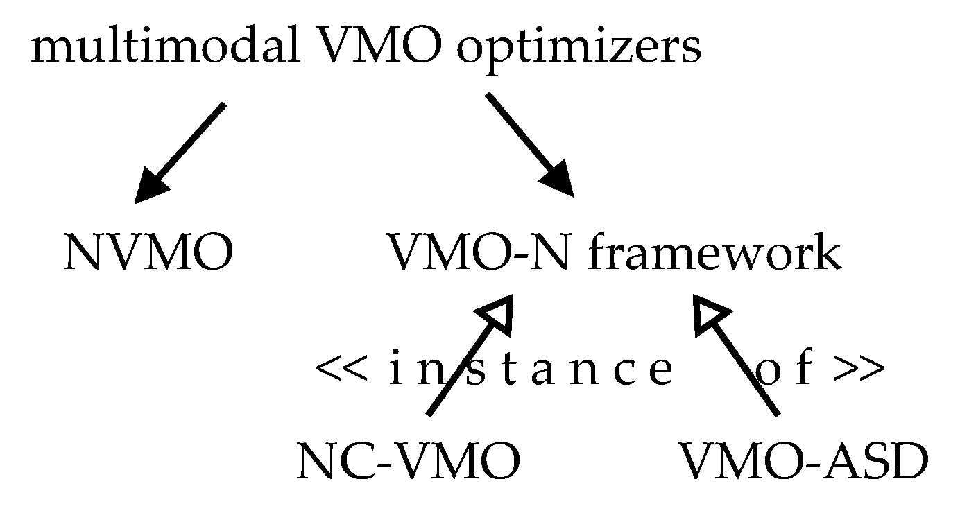
3.4.1. Niching VMO
- With reference to the creation of new nodes from a global perspective, not only the fittest one in the population is considered for expanding the mesh. Instead, several globally best nodes are determined as those having a fitness value very similar to the best solution. Consequently, a new solution is created between every non-optimal node in the mesh and its nearest node (according to the Euclidean distance) among those marked as global optima.
- In order to improve the search capability of the metaheuristic, the Solis-West local search method [39] is run over only a certain number of nodes from the expanded mesh . The solutions selected are those located more distant from the globally fittest nodes found.
- The globally fittest nodes are kept in an external memory, whose update involves every . If has a ‘visibly’ better (>10−6) fitness than the global optimum saved, the memory restarts with only . Otherwise, means a candidate global optimum if it is ‘similar’ (±10−6) in fitness to the global optimum. In that case, the memory accepts if its closest global optima is located at a least distance denoted as the memory threshold (assumed in [23] as the accuracy level [40]).
3.4.2. VMO with Niching
3.4.3. Divergence between VMO-N and NVMO
3.5. Hill-Valley Evolutionary Algorithm
3.5.1. Hill-Valley Function: A Pivotal Subject for HillVallEA
3.5.2. Hill-Valley Clustering: The Niching Method
3.5.3. AMaLGaM-Univariate: The Core Search Method
3.5.4. Elitist Archive, Restart Scheme and Overall Process
| Algorithm 3 HillVallEA | ||
| Inputs: | -dimensional problem as in Section 2, plus the following main parameters: | |
| : the core search algorithm (e.g. AMaLGaM-Univariate) | ||
| : population size (in HillVallEA19: 64; in HillVallEA18: ) | ||
| : increment factor for the population size (suggested value: 2.0) | ||
| : recommended population size for (for AMaLGaM-Univariate: ) | ||
| : initial fraction of the population size of (in HillVallEA19: 0.8; in HillVallEA18: 1.0) | ||
| : increment factor for population size of (in HillVallEA19: 1.1; in HillVallEA18: 1.2) | ||
| : selection fraction for (for AMaLGaM-Univariate: 0.35) | ||
| : tolerance (by default: ; it may be set equal to the accuracy level) | ||
| : budget expressed as the Maximum number of Function Evaluations | ||
| Process: | ||
| 1. | // Actual population size for | |
| 2. | ||
| 3. | // Elitist archive | |
| 4. | ||
| 5. | while do | // Enough to prepare solutions? |
| 6. | ||
| 7. | // Population backup | |
| 8. | ||
| 9. | // Portion of said by | |
| 10. | ||
| 11. | ||
| 12. | // Set of candidate global optima | |
| 13. | for to do | |
| 14. | if then | // If the master of is not a prior elite, |
| 15. | // run to enhance that niche; take the | |
| 16. | // fittest solution as a candidate optimum | |
| 17. | end if | |
| 18. | end for | |
| 19. | // Count elites either replaced or added | |
| 20. | if then | |
| 21. | // If remains unaltered, increase | |
| 22. | // both population sizes | |
| 23. | end if | |
| 24. | end while | |
| Output: | ||
| 25. | return | |
3.6. Research Objectives
- (1)
- To compare VMO-N and NVMO from a conceptual perspective
- (2)
- To revise the VMO-N framework
- (3)
- To create a competitive variant of VMO-N
- (4)
- To decrease the running time of HillVallEA while keeping it effective
- (5)
- To find guidelines to select between past and new methods to better solve additional problems
4. The Proposals
4.1. Variable Mesh Optimization with Niching: A Revised Framework

4.2. Hill-Valley-Clustering-Based Variable Mesh Optimization
- two external lists are used to keep the elites and those nodes for rejection, respectively,
- HVC is employed as the niching algorithm,
- the adaptive clearing is not applied,
- a local optimizer is run over each niche, and
- the mesh in the next generation is fully replaced by a new one.

- Hypothesis 1: Using additional search operators to enhance the population before niching may reduce the total number of solutions throughout the optimization process by HillVallEA.
- Hypothesis 2: If the reduction of the overall number of solutions is big enough, the total execution time of HillVallEA should also decrease, while keeping quite similar multimodal capability.
5. Experimental Setup
5.1. Configuration of Parameters of HVcMO20a
5.2. Benchmark Multimodal Problems
5.3. Baseline Methods
5.4. Major Performance Criteria
5.5. Statistical Validation
6. Discussion of Results
6.1. Outperforming NVMO and Earlier Instances of VMO-N
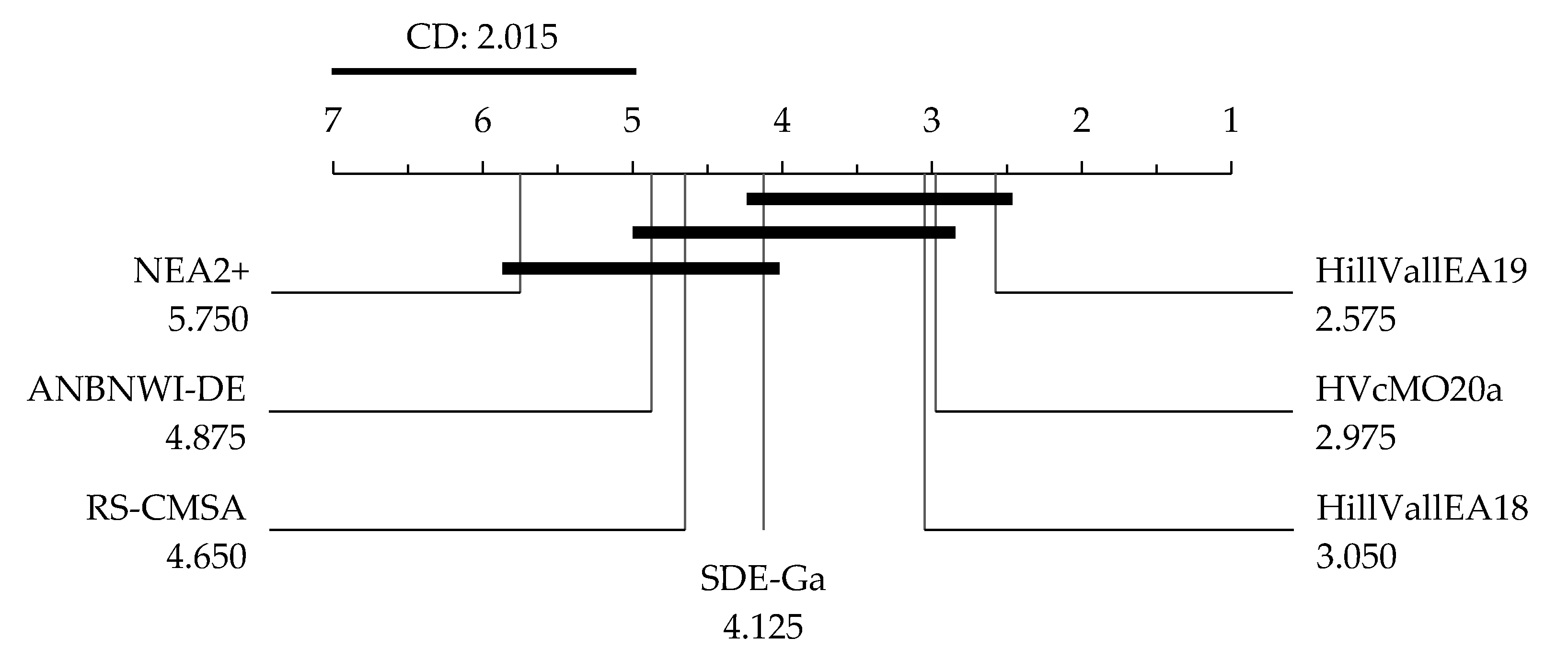
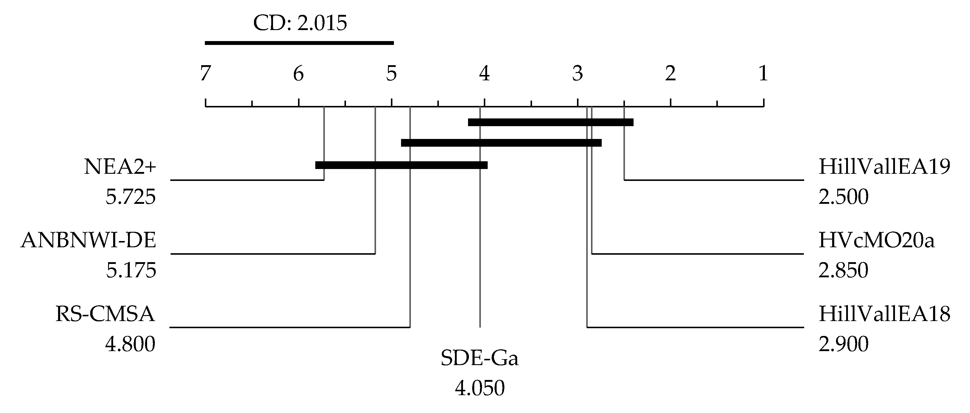
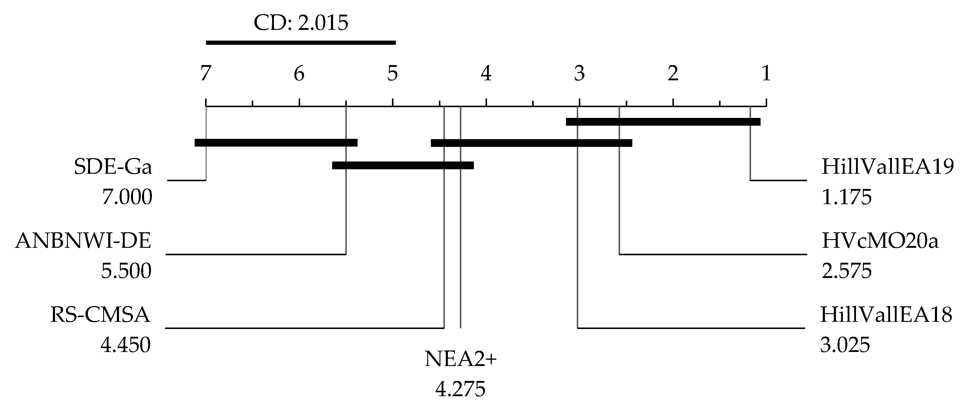
6.2. Further Baseline Comparison
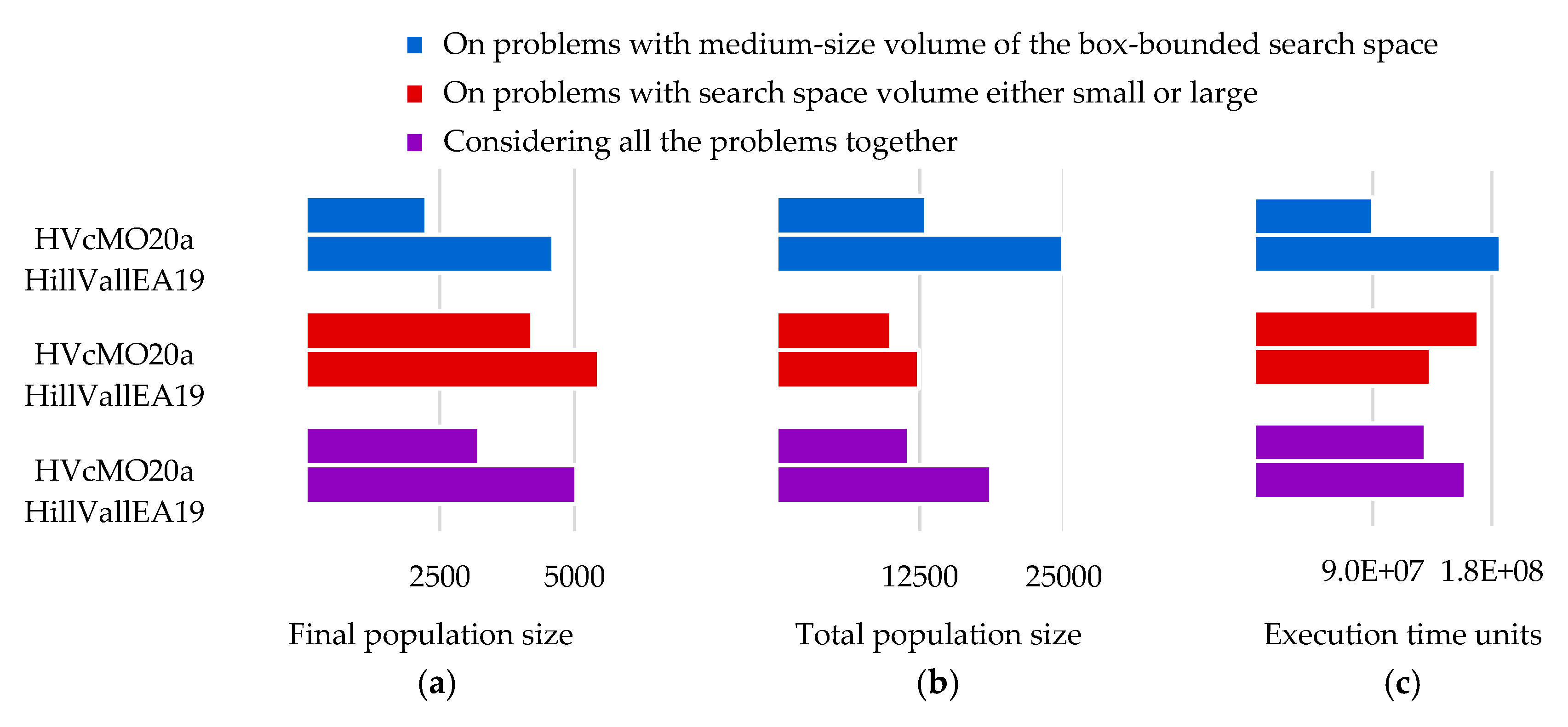
6.3. HVcMO20a or HillVallEA19? When to Apply Each?
6.3.1. When Counting Function Evaluations Is Not Enough
- executing single iterations of them, instead of the whole evolutionary process,
- conducting the experiment over populations of certain sizes, to be exact ,
- generating 50 distinct populations for every single sample size,
- running the programs over each of the 20 benchmark problems using the same populations,
- replicating the process for five levels of tolerance set equal to the accuracy levels, for a total of 25,000 runs per program (the tolerance influences AMaLGaM-Univariate and thus, the overall process),
- effecting the 50,000 runs in turn and on the same computer, i.e., using the same specifications of hardware and software,
- operating no other computational process, apart from those controlled by the system,
- reusing much of the source code of HillVallEA19 to program the common aspects in HVcMO20a, to reduce the influence that the skills of the programmer have over the execution time, and by
- estimating the ratio based not only on mean calculations but also on every single paired contrast,
- excluding the outliers during the examination of the resultant measurements.
6.3.2. The Time Ratio
6.3.3. Population Size and Execution Time
7. Conclusions and Future Work
Supplementary Materials
Author Contributions
Funding
Acknowledgments
Conflicts of Interest
Appendix A. PR, F1 and dynF1

| Problem | ANBNWI-DE | HillVallEA19 | HVcMO20a | ||||||
|---|---|---|---|---|---|---|---|---|---|
| Id | PR | F1 | dynF1 | PR | F1 | dynF1 | PR | F1 | dynF1 |
| 1 | 1.000 | 1.000 | 0.974 | 1.000 | 1.000 | 0.995 | 1.000 | 1.000 | 0.993 |
| 2 | 0.998 | 0.998 | 0.972 | 1.000 | 1.000 | 0.989 | 1.000 | 1.000 | 0.986 |
| 3 | 1.000 | 0.667 | 0.650 | 1.000 | 1.000 | 0.994 | 1.000 | 1.000 | 0.991 |
| 4 | 0.996 | 0.996 | 0.952 | 1.000 | 1.000 | 0.976 | 1.000 | 1.000 | 0.973 |
| 5 | 1.000 | 1.000 | 0.968 | 1.000 | 1.000 | 0.984 | 1.000 | 1.000 | 0.983 |
| 6 | 1.000 | 1.000 | 0.625 | 1.000 | 1.000 | 0.967 | 1.000 | 1.000 | 0.956 |
| 7 | 0.965 | 0.977 | 0.871 | 1.000 | 1.000 | 0.966 | 1.000 | 1.000 | 0.963 |
| 8 | 0.925 | 0.960 | 0.587 | 0.979 | 0.989 | 0.806 | 0.974 | 0.986 | 0.797 |
| 9 | 0.692 | 0.812 | 0.555 | 0.968 | 0.984 | 0.810 | 0.951 | 0.975 | 0.803 |
| 10 | 0.999 | 0.999 | 0.981 | 1.000 | 1.000 | 0.982 | 1.000 | 1.000 | 0.980 |
| 11 | 0.995 | 0.968 | 0.885 | 1.000 | 1.000 | 0.983 | 1.000 | 1.000 | 0.981 |
| 12 | 0.925 | 0.947 | 0.649 | 1.000 | 1.000 | 0.964 | 1.000 | 1.000 | 0.958 |
| 13 | 1.000 | 0.986 | 0.866 | 1.000 | 1.000 | 0.963 | 1.000 | 1.000 | 0.948 |
| 14 | 0.889 | 0.922 | 0.787 | 0.923 | 0.958 | 0.881 | 0.847 | 0.913 | 0.851 |
| 15 | 0.738 | 0.848 | 0.623 | 0.750 | 0.857 | 0.837 | 0.750 | 0.857 | 0.829 |
| 16 | 0.683 | 0.804 | 0.662 | 0.694 | 0.817 | 0.791 | 0.667 | 0.800 | 0.783 |
| 17 | 0.666 | 0.797 | 0.486 | 0.750 | 0.857 | 0.815 | 0.750 | 0.857 | 0.803 |
| 18 | 0.667 | 0.800 | 0.633 | 0.667 | 0.800 | 0.765 | 0.667 | 0.800 | 0.762 |
| 19 | 0.550 | 0.708 | 0.464 | 0.595 | 0.743 | 0.660 | 0.608 | 0.753 | 0.659 |
| 20 | 0.402 | 0.555 | 0.347 | 0.483 | 0.650 | 0.529 | 0.488 | 0.655 | 0.528 |
Appendix B. Ratio of Time and Population Size
| All Pop Sizes | ||||||||||||
|---|---|---|---|---|---|---|---|---|---|---|---|---|
| Problem | RoM | MoR | RoM | MoR | RoM | MoR | RoM | MoR | RoM | MoR | RoM | MoR |
| Id | Considering 50 Runs per Function Using a Tolerance of | |||||||||||
| 1 | 1.343 | 1.354 | 1.346 | 1.351 | 1.330 | 1.330 | 1.342 | 1.342 | 1.321 | 1.321 | 1.325 | 1.340 |
| 2 | 1.250 | 1.281 | 1.363 | 1.369 | 1.301 | 1.304 | 1.334 | 1.342 | 1.319 | 1.319 | 1.321 | 1.323 |
| 3 | 1.305 | 1.327 | 1.375 | 1.382 | 1.324 | 1.324 | 1.354 | 1.354 | 1.316 | 1.316 | 1.324 | 1.341 |
| 4 | 1.166 | 1.189 | 1.287 | 1.293 | 1.282 | 1.283 | 1.340 | 1.340 | 1.311 | 1.311 | 1.314 | 1.283 |
| 5 | 1.196 | 1.221 | 1.309 | 1.315 | 1.294 | 1.296 | 1.350 | 1.350 | 1.313 | 1.313 | 1.318 | 1.299 |
| 6 | 1.362 | 1.382 | 1.440 | 1.451 | 1.459 | 1.460 | 1.373 | 1.373 | 1.312 | 1.312 | 1.335 | 1.396 |
| 7 | 1.311 | 1.330 | 1.333 | 1.344 | 1.339 | 1.340 | 1.332 | 1.332 | 1.308 | 1.309 | 1.315 | 1.331 |
| 8 | 1.480 | 1.525 | 1.427 | 1.442 | 1.488 | 1.489 | 1.430 | 1.431 | 1.372 | 1.372 | 1.393 | 1.452 |
| 9 | 1.616 | 1.635 | 1.454 | 1.460 | 1.417 | 1.419 | 1.356 | 1.357 | 1.296 | 1.300 | 1.325 | 1.434 |
| 10 | 1.093 | 1.108 | 1.211 | 1.215 | 1.260 | 1.260 | 1.334 | 1.334 | 1.319 | 1.319 | 1.314 | 1.247 |
| 11 | 1.124 | 1.141 | 1.233 | 1.238 | 1.276 | 1.278 | 1.355 | 1.356 | 1.326 | 1.326 | 1.322 | 1.268 |
| 12 | 1.406 | 1.431 | 1.451 | 1.471 | 1.404 | 1.406 | 1.380 | 1.380 | 1.315 | 1.315 | 1.339 | 1.401 |
| 13 | 1.265 | 1.304 | 1.390 | 1.397 | 1.358 | 1.359 | 1.397 | 1.397 | 1.341 | 1.341 | 1.353 | 1.360 |
| 14 | 1.296 | 1.313 | 1.389 | 1.398 | 1.438 | 1.444 | 1.486 | 1.487 | 1.380 | 1.381 | 1.403 | 1.405 |
| 15 | 1.372 | 1.443 | 1.536 | 1.562 | 1.465 | 1.475 | 1.468 | 1.469 | 1.386 | 1.391 | 1.412 | 1.468 |
| 16 | 1.266 | 1.316 | 1.256 | 1.288 | 1.341 | 1.350 | 1.418 | 1.420 | 1.386 | 1.386 | 1.378 | 1.352 |
| 17 | 1.265 | 1.309 | 1.306 | 1.338 | 1.439 | 1.455 | 1.443 | 1.446 | 1.388 | 1.389 | 1.396 | 1.387 |
| 18 | 1.049 | 1.126 | 1.020 | 1.068 | 1.083 | 1.098 | 1.200 | 1.208 | 1.233 | 1.236 | 1.185 | 1.147 |
| 19 | 1.094 | 1.141 | 1.073 | 1.114 | 1.131 | 1.147 | 1.201 | 1.211 | 1.237 | 1.240 | 1.194 | 1.171 |
| 20 | 1.010 | 1.112 | 0.939 | 0.991 | 1.000 | 1.036 | 1.097 | 1.123 | 1.182 | 1.186 | 1.088 | 1.090 |
| Id | Considering 250 Runs per Function: 50 Runs for Every Mesh Size Using the 5 Levels of Tolerance | |||||||||||
| 1 | 1.370 | 1.387 | 1.347 | 1.352 | 1.360 | 1.360 | 1.343 | 1.343 | 1.333 | 1.334 | 1.336 | 1.355 |
| 2 | 1.318 | 1.342 | 1.351 | 1.355 | 1.339 | 1.342 | 1.332 | 1.338 | 1.341 | 1.341 | 1.339 | 1.344 |
| 3 | 1.371 | 1.394 | 1.336 | 1.343 | 1.362 | 1.363 | 1.331 | 1.332 | 1.342 | 1.342 | 1.341 | 1.355 |
| 4 | 1.236 | 1.254 | 1.287 | 1.291 | 1.329 | 1.331 | 1.328 | 1.328 | 1.337 | 1.337 | 1.333 | 1.308 |
| 5 | 1.202 | 1.229 | 1.311 | 1.316 | 1.331 | 1.335 | 1.337 | 1.337 | 1.328 | 1.328 | 1.329 | 1.309 |
| 6 | 1.394 | 1.422 | 1.438 | 1.448 | 1.470 | 1.472 | 1.364 | 1.364 | 1.335 | 1.336 | 1.350 | 1.408 |
| 7 | 1.358 | 1.378 | 1.344 | 1.352 | 1.344 | 1.345 | 1.310 | 1.312 | 1.324 | 1.326 | 1.323 | 1.343 |
| 8 | 1.480 | 1.527 | 1.451 | 1.465 | 1.492 | 1.494 | 1.414 | 1.415 | 1.385 | 1.385 | 1.400 | 1.457 |
| 9 | 1.609 | 1.626 | 1.450 | 1.457 | 1.432 | 1.434 | 1.342 | 1.343 | 1.317 | 1.318 | 1.338 | 1.436 |
| 10 | 1.142 | 1.156 | 1.200 | 1.204 | 1.287 | 1.290 | 1.316 | 1.317 | 1.331 | 1.331 | 1.321 | 1.259 |
| 11 | 1.137 | 1.158 | 1.211 | 1.217 | 1.309 | 1.311 | 1.337 | 1.338 | 1.344 | 1.344 | 1.334 | 1.273 |
| 12 | 1.408 | 1.437 | 1.445 | 1.464 | 1.446 | 1.449 | 1.360 | 1.360 | 1.343 | 1.343 | 1.356 | 1.411 |
| 13 | 1.270 | 1.308 | 1.368 | 1.374 | 1.392 | 1.394 | 1.373 | 1.375 | 1.355 | 1.356 | 1.360 | 1.361 |
| 14 | 1.269 | 1.288 | 1.389 | 1.399 | 1.474 | 1.479 | 1.464 | 1.465 | 1.395 | 1.397 | 1.411 | 1.405 |
| 15 | 1.340 | 1.392 | 1.498 | 1.523 | 1.495 | 1.503 | 1.453 | 1.454 | 1.407 | 1.409 | 1.424 | 1.456 |
| 16 | 1.254 | 1.301 | 1.249 | 1.274 | 1.355 | 1.367 | 1.399 | 1.401 | 1.388 | 1.389 | 1.376 | 1.346 |
| 17 | 1.263 | 1.308 | 1.274 | 1.301 | 1.425 | 1.443 | 1.414 | 1.418 | 1.402 | 1.402 | 1.396 | 1.374 |
| 18 | 0.956 | 1.047 | 1.029 | 1.098 | 1.103 | 1.120 | 1.198 | 1.206 | 1.232 | 1.235 | 1.182 | 1.141 |
| 19 | 1.022 | 1.051 | 1.011 | 1.049 | 1.134 | 1.150 | 1.185 | 1.195 | 1.248 | 1.250 | 1.187 | 1.139 |
| 20 | 1.002 | 1.100 | 0.945 | 0.993 | 1.023 | 1.064 | 1.079 | 1.104 | 1.187 | 1.192 | 1.089 | 1.091 |
| All Sizes | Percentage Covered | ||||||||
|---|---|---|---|---|---|---|---|---|---|
| tratio ∊ | For Every Population Size: 50 Runs per Each of 20 Functions for Tolerance | ||||||||
| (0.00, 1.00] | 161 | 89 | 53 | 21 | 3 | 327 | 6.54% | ||
| (1.00, 1.20] | 237 | 162 | 80 | 66 | 63 | 608 | 12.16% | } | 27.52% |
| (1.20, 1.30] | 150 | 183 | 243 | 55 | 137 | 768 | 15.36% | ||
| (1.30, 1.40] | 113 | 223 | 352 | 601 | 722 | 2011 | 40.22% | } | 60.84% |
| (1.40, 1.65] | 206 | 258 | 243 | 251 | 73 | 1031 | 20.62% | ||
| (1.65, 1.75] | 44 | 44 | 13 | 6 | 0 | 107 | 2.14% | } | 4.16% |
| (1.75, 2.00] | 57 | 29 | 13 | 0 | 2 | 101 | 2.02% | ||
| (2.00, 2.50] | 26 | 11 | 3 | 0 | 0 | 40 | 0.80% | } | 0.94% |
| (2.50, 4.00] | 6 | 1 | 0 | 0 | 0 | 7 | 0.14% | ||
| #Runs | 1000 | 1000 | 1000 | 1000 | 1000 | 5000 | |||
| tratio ∊ | For Every Population Size: 50 per Each of 20 Functions Using the 5 Levels of Tolerance | ||||||||
| (0.00, 1.00] | 777 | 435 | 244 | 104 | 16 | 1576 | 6.30% | ||
| (1.00, 1.20] | 1185 | 882 | 386 | 354 | 273 | 3080 | 12.32% | } | 26.43% |
| (1.20, 1.30] | 686 | 942 | 710 | 591 | 598 | 3527 | 14.11% | ||
| (1.30, 1.40] | 631 | 1140 | 1958 | 2881 | 3500 | 10,110 | 40.44% | } | 62.12% |
| (1.40, 1.65] | 1035 | 1231 | 1512 | 1038 | 605 | 5421 | 21.68% | ||
| (1.65, 1.75] | 209 | 179 | 105 | 24 | 0 | 517 | 2.07% | } | 4.21% |
| (1.75, 2.00] | 313 | 140 | 68 | 7 | 6 | 534 | 2.14% | ||
| (2.00, 2.50] | 150 | 47 | 17 | 1 | 2 | 217 | 0.87% | } | 0.94% |
| (2.50, 4.00] | 14 | 4 | 0 | 0 | 0 | 18 | 0.07% | ||
| #Runs | 5000 | 5000 | 5000 | 5000 | 5000 | 25,000 | |||
| Problem | Final Pop Size (Actual) | Total Pop Size (Actual) | Time Units (Estimated) | |||
|---|---|---|---|---|---|---|
| Id | HVcMO20a | HillVallEA19 | HVcMO20a | HillVallEA19 | HVcMO20a | HillVallEA19 |
| 1 | 65 | 64 | 137 | 128 | 18,186 | 8192 |
| 2 | 64 | 64 | 131 | 134 | 16,712 | 8602 |
| 3 | 64 | 64 | 128 | 128 | 16,384 | 8192 |
| 4 | 68 | 77 | 159 | 197 | 22,282 | 15,892 |
| 5 | 64 | 64 | 129 | 132 | 16,548 | 8438 |
| 6 | 302 | 461 | 1437 | 2198 | 777,748 | 883,671 |
| 7 | 1546 | 2929 | 7350 | 13,545 | 18,752,143 | 32,556,974 |
| 8 | 901 | 2191 | 7578 | 16,497 | 6,688,968 | 16,971,203 |
| 9 | 7946 | 19,988 | 85,183 | 165,129 | 700,629,722 | 1,529,669,468 |
| 10 | 68 | 70 | 187 | 223 | 25,887 | 15,892 |
| 11 | 252 | 358 | 868 | 1179 | 493,158 | 539,935 |
| 12 | 316 | 637 | 1230 | 2388 | 811,500 | 1,642,824 |
| 13 | 1341 | 1920 | 4429 | 6348 | 12,453,151 | 13,276,692 |
| 14 | 5714 | 9380 | 13,559 | 24,901 | 114,926,086 | 179,571,917 |
| 15 | 4096 | 8192 | 8893 | 17,299 | 45,454,131 | 90,031,473 |
| 16 | 6636 | 8192 | 13,509 | 16,721 | 128,647,938 | 90,269,860 |
| 17 | 4096 | 8192 | 8995 | 17,318 | 45,485,425 | 89,991,086 |
| 18 | 4096 | 4588 | 8504 | 9468 | 44,906,250 | 30,494,802 |
| 19 | 8028 | 8684 | 18,258 | 19,988 | 185,760,922 | 115,860,931 |
| 20 | 19,005 | 24,576 | 50,104 | 59,748 | 1,294,673,004 | 1,010,064,589 |
References
- Reeves, C.R. Modern Heuristic Techniques. In Modern heuristic search methods; Rayward-Smith, V.J., Osman, I.H., Reeves, C.R., Smith, G.D., Eds.; John Wiley & Sons: New York, NY, USA, 1996; pp. 1–25. [Google Scholar]
- Sörensen, K.; Sevaux, M.; Glover, F. A History of Metaheuristics. In Handbook of Heuristics; Martí, R., Pardalos, P.M., Resende, M.G., Eds.; Springer: Cham, Switzerland, 2018; pp. 1–18. [Google Scholar] [CrossRef]
- Chica, M.; Barranquero, J.; Kajdanowicz, T.; Damas, S.; Cordón, Ó. Multimodal optimization: An effective framework for model calibration. Inf. Sci. 2017, 375, 79–97. [Google Scholar] [CrossRef]
- Woo, D.-K.; Choi, J.-H.; Ali, M.; Jung, H.-K. A Novel Multimodal Optimization Algorithm Applied to Electromagnetic Optimization. IEEE Trans. Magn. 2011, 47, 1667–1673. [Google Scholar] [CrossRef]
- Dilettoso, E.; Salerno, N. A Self-Adaptive Niching Genetic Algorithm for Multimodal Optimization of Electromagnetic Devices. IEEE Trans. Magn. 2006, 42, 1203–1206. [Google Scholar] [CrossRef]
- Das, S.; Maity, S.; Qu, B.-Y.; Suganthan, P.N. Real-Parameter Evolutionary Multimodal Optimization-A Survey of the State-of-the-Art. Swarm Evol. Comput. 2011, 2, 71–88. [Google Scholar] [CrossRef]
- Della Cioppa, A.; De Stefano, C.; Marcelli, A. Where Are the Niches? Dynamic Fitness Sharing. IEEE Trans. Evol. Comput. 2007, 11, 453–465. [Google Scholar] [CrossRef]
- Kamyab, S.; Eftekhari, M. Using a Self-Adaptive Neighborhood Scheme with Crowding Replacement Memory in Genetic Algorithm for Multimodal Optimization. Swarm Evol. Comput. 2013, 12, 1–17. [Google Scholar] [CrossRef]
- Sopov, E. Self-Configuring Ensemble of Multimodal Genetic Algorithms. In Computational Intelligence. IJCCI 2015. Studies in Computational Intelligence, Vol 669; Merelo, J.J., Rosa, A., Cadenas, J.M., Correia, A.D., Madani, K., Ruano, A., Filipe, J., Eds.; Springer: Cham, Switzerland, 2017; pp. 56–74. [Google Scholar] [CrossRef]
- De Magalhães, C.S.; Almeida, D.M.; Barbosa, H.J.C.; Dardenne, L.E. A Dynamic Niching Genetic Algorithm Strategy for Docking Highly Flexible Ligands. Inf. Sci. 2014, 289, 206–224. [Google Scholar] [CrossRef]
- Li, X. Niching Without Niching Parameters: Particle Swarm Optimization Using a Ring Topology. IEEE Trans. Evol. Comput. 2010, 14, 150–169. [Google Scholar] [CrossRef]
- Nápoles, G.; Grau, I.; Bello, R.; Falcon, R.; Abraham, A. Self-Adaptive Differential Particle Swarm Using a Ring Topology for Multimodal Optimization. In Proceedings of the 13th International Conference on Intelligent Systems Design and Applications (ISDA’13), Bangi, Malaysia, 8–10 December 2013; pp. 35–40. [Google Scholar] [CrossRef]
- Fieldsend, J.E. Running Up Those Hills: Multi-Modal Search with the Niching Migratory Multi-Swarm Optimiser. In Proceedings of the 2014 IEEE Congress on Evolutionary Computation (CEC’14), Beijing, China, 6–11 July 2014; pp. 2593–2600. [Google Scholar] [CrossRef]
- Li, X. Developing Niching Algorithms in Particle Swarm Optimization. In Handbook of Swarm Intelligence. Adaptation, Learning, and Optimization; Panigrahi, B.K., Shi, Y., Lim, M.-H., Eds.; Springer: Berlin/Heidelberg, Germany, 2011; Volume 8, pp. 67–88. [Google Scholar] [CrossRef]
- Qu, B.Y.; Suganthan, P.N. Novel Multimodal Problems and Differential Evolution with Ensemble of Restricted Tournament Selection. In Proceedings of the 2010 IEEE Congress on Evolutionary Computation (CEC’10), Barcelona, Spain, 18–23 July 2010; pp. 1–7. [Google Scholar] [CrossRef]
- Epitropakis, M.G.; Plagianakos, V.P.; Vrahatis, M.N. Finding Multiple Global Optima Exploiting Differential Evolution’s Niching Capability. In Proceedings of the 2011 IEEE Symposium on Differential Evolution (SDE’11), Paris, France, 11–15 April 2011; pp. 1–8. [Google Scholar] [CrossRef]
- Thomsen, R. Multimodal Optimization Using Crowding-Based Differential Evolution. In Proceedings of the 2004 IEEE Congress on Evolutionary Computation (CEC’04), Portland, OR, USA, 19–23 June 2004; Volume 2, pp. 1382–1389. [Google Scholar] [CrossRef]
- Epitropakis, M.G.; Li, X.; Burke, E.K. A Dynamic Archive Niching Differential Evolution Algorithm for Multimodal Optimization. In Proceedings of the 2013 IEEE Congress on Evolutionary Computation (CEC’13), Cancún, Mexico, 20–23 June 2013; pp. 79–86. [Google Scholar] [CrossRef]
- Shir, O.M. Niching in Evolutionary Algorithms. In Handbook of Natural Computing; Rozenberg, G., Bäck, T., Kok, J.N., Eds.; Springer: Berlin/Heidelberg, Germany, 2012; pp. 1035–1069. [Google Scholar] [CrossRef]
- Puris, A.; Bello, R.; Molina, D.; Herrera, F. Variable Mesh Optimization for Continuous Optimization Problems. Soft Comput. 2012, 16, 511–525. [Google Scholar] [CrossRef]
- Navarro, R.; Falcon, R.; Bello, R.; Abraham, A. Niche-Clearing-Based Variable Mesh Optimization for Multimodal Problems. In Proceedings of the 2013 World Congress on Nature and Biologically Inspired Computing (NaBIC’13), Fargo, ND, USA, 12–14 August 2013; pp. 161–168. [Google Scholar] [CrossRef]
- Navarro, R.; Murata, T.; Falcon, R.; Kim, C.H. A Generic Niching Framework for Variable Mesh Optimization. In Proceedings of the 2015 IEEE Congress on Evolutionary Computation (CEC’15), Sendai, Japan, 25–28 May 2015; pp. 1994–2001. [Google Scholar] [CrossRef]
- Molina, D.; Puris, A.; Bello, R.; Herrera, F. Variable Mesh Optimization for the 2013 CEC Special Session Niching Methods for Multimodal Optimization. In Proceedings of the 2013 IEEE Congress on Evolutionary Computation (CEC’13), Cancún, Mexico, 20–23 June 2013; pp. 87–94. [Google Scholar] [CrossRef]
- Maree, S.C.; Thierens, D.; Alderliesten, T.; Bosman, P.A.N. Real-Valued Evolutionary Multi-Modal Optimization Driven by Hill-Valley Clustering. In Proceedings of the 2018 Genetic and Evolutionary Computation Conference (GECCO’18), Kyoto, Japan, 15–19 July 2018; pp. 857–864. [Google Scholar] [CrossRef]
- Bosman, P.A.N.; Grahl, J.; Thierens, D. Enhancing the Performance of Maximum–Likelihood Gaussian EDAs Using Anticipated Mean Shift. In Parallel Problem Solving from Nature—PPSN X. PPSN 2008; Lecture Notes in Computer Science; Rudolph, G., Jansen, T., Beume, N., Lucas, S., Poloni, C., Eds.; Springer: Berlin/Heidelberg, Germany, 2008; Volume 5199, pp. 133–143. [Google Scholar] [CrossRef]
- Bosman, P.A.N.; Grahl, J.; Thierens, D. Benchmarking Parameter-Free AMaLGaM on Functions With and Without Noise. Evol. Comput. 2013, 21, 445–469. [Google Scholar] [CrossRef] [PubMed]
- Maree, S.C.; Alderliesten, T.; Bosman, P.A.N. Benchmarking HillVallEA for the GECCO 2019 Competition on Multimodal Optimization. Available online: https://arxiv.org/abs/1907.10988v1 (accessed on 25 October 2019).
- Competition on Niching Methods for Multimodal Optimization. Available online: http://www.epitropakis.co.uk/gecco2019/ (accessed on 23 October 2019).
- Kanemitsu, H.; Imai, H.; Miyaskoshi, M. Definitions and Properties of (Local) Minima and Multimodal Functions using Level Set for Continuous Optimization Problems. In Proceedings of the 2013 International Symposium on Nonlinear Theory and its Applications (NOLTA2013), Santa Fe, NM, USA, 8–11 September 2013; pp. 94–97. [Google Scholar] [CrossRef]
- Zhai, Z.; Li, X. A Dynamic Archive Based Niching Particle Swarm Optimizer Using a Small Population Size. In Proceedings of the This paper appeared at the Thirty-Fourth Australasian Computer Science Conference (ACSC2011), Perth, Australia, 17 January 2011; Reynolds, M., Ed.; Conferences in Research and Practice in Information Technology (CRPIT), Australian, Computer Society, Inc.: Perth, Australia, 2011; Volume 113. [Google Scholar]
- Kronfeld, M.; Zell, A. Towards Scalability in Niching Methods. In Proceedings of the 2010 IEEE Congress on Evolutionary Computation (CEC’10), Barcelona, Spain, 18–23 July 2010; pp. 1–8. [Google Scholar] [CrossRef]
- Puris, A.; Bello, R.; Molina, D.; Herrera, F. Optimising Real Parameters Using the Information of a Mesh of Solutions: VMO Algorithm. In Proceedings of the 2012 IEEE Congress on Evolutionary Computation (CEC’12), Brisbane, QLD, Australia, 10–15 June 2012; pp. 1–7. [Google Scholar] [CrossRef]
- Pétrowski, A. Clearing Procedure as a Niching Method for Genetic Algorithms. In Proceedings of the IEEE Conference on Evolutionary Computation, Nagoya, Japan, 20–22 May 1996; pp. 798–803. [Google Scholar] [CrossRef]
- Sareni, B.; Krähenbühl, L. Fitness Sharing and Niching Methods Revisited. IEEE Trans. Evol. Comput. 1998, 2, 97–106. [Google Scholar] [CrossRef]
- Li, J.P.; Balazs, M.E.; Parks, G.T.; Clarkson, P.J. A Species Conserving Genetic Algorithm for Multimodal Function Optimization. Evol. Comput. 2002, 10, 207–234. [Google Scholar] [CrossRef] [PubMed]
- Gan, J.; Warwick, K. Dynamic Niche Clustering: A Fuzzy Variable Radius Niching Technique for Multimodal Optimisation in GAs. In Proceedings of the 2001 Congress on Evolutionary Computation (IEEE Cat. No.01TH8546), Seoul, Korea, 27–30 May 2001; Volume 1, pp. 215–222. [Google Scholar] [CrossRef]
- Brown, M.S. A Species-Conserving Genetic Algorithm for Multimodal Optimization; Nova Southeastern University: Fort Lauderdale, FL, USA, 2010. [Google Scholar]
- Iwase, T.; Takano, R.; Uwano, F.; Sato, H.; Takadama, K. The Bat Algorithm with Dynamic Niche Radius for Multimodal Optimization. In Proceedings of the 2019 3rd International Conference on Intelligent Systems, Metaheuristics & Swarm Intelligence, Malé, Maldives, 24 March 2019; pp. 8–13. [Google Scholar] [CrossRef]
- Solis, F.J.; Wets, R.J.B. Minimization by Random Search Techniques. Math. Oper. Res. 1981, 6, 19–30. [Google Scholar] [CrossRef]
- Li, X.; Engelbrecht, A.; Epitropakis, M.G. Benchmark Functions for CEC’2013 Special Session and Competition on Niching Methods for Multimodal Function Optimization. Technical Report. Evolutionary Computation and Machine Learning Group, RMIT University: Australia, 2013. Available online: https://titan.csit.rmit.edu.au/~e46507/cec13-niching/competition/cec2013-niching-benchmark-tech-report.pdf (accessed on 23 October 2019).
- Qu, B.Y.; Liang, J.J.; Suganthan, P.N. Niching Particle Swarm Optimization with Local Search for Multi-Modal Optimization. Inf. Sci. 2012, 197, 131–143. [Google Scholar] [CrossRef]
- Della Cioppa, A.; Marcelli, A.; Napoli, P. Speciation in Evolutionary Algorithms: Adaptive Species Discovery. In Proceedings of the 2011 Genetic and Evolutionary Computation Conference (GECCO’11), Dublin, Ireland, 12 July 2011; pp. 1053–1060. [Google Scholar] [CrossRef]
- Ursem, R.K. Multinational Evolutionary Algorithms. In Proceedings of the 1999 Congress on Evolutionary Computation-CEC99 (Cat. No. 99TH8406), Washington, DC, USA, 6–9 July 1999; Volume 3, pp. 1633–1640. [Google Scholar] [CrossRef]
- Towards a New Evolutionary Computation. Studies in Fuzziness and Soft Computing; Lozano, J.A., Larrañaga, P., Inza, I., Bengoetxea, E., Eds.; Springer: Berlin/Heidelberg, Germany, 2006; Volume 192. [Google Scholar] [CrossRef]
- Dong, W.; Yao, X. NichingEDA: Utilizing the Diversity inside a Population of EDAs for Continuous Optimization. In Proceedings of the 2008 IEEE Congress on Evolutionary Computation (CEC’08), Hong Kong, China, 1–6 June 2008; pp. 1260–1267. [Google Scholar] [CrossRef]
- Chen, B.; Hu, J. An Adaptive Niching EDA Based on Clustering Analysis. In Proceedings of the 2010 IEEE Congress on Evolutionary Computation (CEC’10), Barcelona, Spain, 18–23 July 2010; pp. 1–7. [Google Scholar] [CrossRef]
- Yang, P.; Tang, K.; Lu, X. Improving Estimation of Distribution Algorithm on Multimodal Problems by Detecting Promising Areas. IEEE Trans. Cybern. 2015, 45, 1438–1449. [Google Scholar] [CrossRef] [PubMed]
- HillVallEA. Available online: https://github.com/scmaree/HillVallEA (accessed on 28 October 2019).
- Rodrigues, S.; Bauer, P.; Bosman, P.A.N. A Novel Population-Based Multi-Objective CMA-ES and the Impact of Different Constraint Handling Techniques. In Proceedings of the 2014 Genetic and Evolutionary Computation Conference (GECCO’14), Vancouver, BC, Canada, 12–16 July 2014; pp. 991–998. [Google Scholar] [CrossRef]
- Wolpert, D.H.; Macready, W.G. No Free Lunch Theorems for Optimization. IEEE Trans. Evol. Comput. 1997, 1, 67–82. [Google Scholar] [CrossRef]
- Navarro, R. Optimización Basada En Mallas Variables Con Operador de Fronteras Basado En Búsqueda Genética (Variable Mesh Optimization with Frontiers Operator Based on Genetic Search); Universidad de Holguín: Piedra Blanca, Holguín, Cuba, 2012; Available online: https://repositorio.uho.edu.cu/jspui/handle/uho/444 (accessed on 10 March 2020).
- Preuss, M. Improved Topological Niching for Real-Valued Global Optimization. In Applications of Evolutionary Computation. EvoApplications 2012. Lecture Notes in Computer Science; Springer: Berlin/Heidelberg, Germany, 2012; Volume 7248. [Google Scholar] [CrossRef]
- Ahrari, A.; Deb, K.; Preuss, M. Multimodal Optimization by Covariance Matrix Self-Adaptation Evolution Strategy with Repelling Subpopulations. Evol. Comput. 2017, 25, 439–471. [Google Scholar] [CrossRef] [PubMed]
- CEC2013. Available online: https://github.com/mikeagn/CEC2013 (accessed on 15 January 2020).
- Demšar, J. Statistical Comparisons of Classifiers over Multiple Data Sets. J. Mach. Learn. Res. 2006, 7, 1–30. [Google Scholar]
- Derrac, J.; García, S.; Molina, D.; Herrera, F. A Practical Tutorial on the Use of Nonparametric Statistical Tests as a Methodology for Comparing Evolutionary and Swarm Intelligence Algorithms. Swarm Evol. Comput. 2011, 1, 3–18. [Google Scholar] [CrossRef]
- HVcMO. Available online: https://github.com/ricardonrcu/HVcMO (accessed on 24 March 2020).


| Criteria for Comparison | NVMO | VMO-N Framework |
|---|---|---|
| Algorithmic sequence (core actions in each iteration) | expansion → local search → memory update → adaptive clearing (as niching) | expansion → niching step → adaptive clearing (as for diversity) |
| Maintenance of the globally fittest found solutions | An extra memory is needed to keep such solutions | They are properly kept in the mesh (future variants may save them apart) |
| Formation of niches | The adaptive clearing is taken as a niching method but the masters are not used for multimodal purpose | Any niching method can be incorporated at will |
| Requirement of niching parameters | The computed threshold for the adaptive clearing is used as a dynamic niche radius | It varies, subject to the needs of the niching scheme, e.g., VMO-ASD is free of such parameters but NC-VMO uses a niche radius |
| Effecting of the adaptive clearing of VMO | It affects the whole mesh at once | It is executed, by separate, over each identified niche |
| Utilization of local search | The Solis-West method is used, in order to strengthen the search ability | No local search technique is applied (future instances may consider it) |
| Applicability | It can be applied to approximate a large range of multimodal problems | For each case, it relies mainly on the niching method, e.g., VMO-ASD is widely applicable; NC-VMO is not |
| Id | f | Name | D | Domain Bounds | Vol | #GOpt | #LOpt | MaxFE |
|---|---|---|---|---|---|---|---|---|
| 1 | F1(x) | Five-Uneven-Peak Trap | 1 | x ∊ [0, 30] | 30.00 | 2 | 3 | |
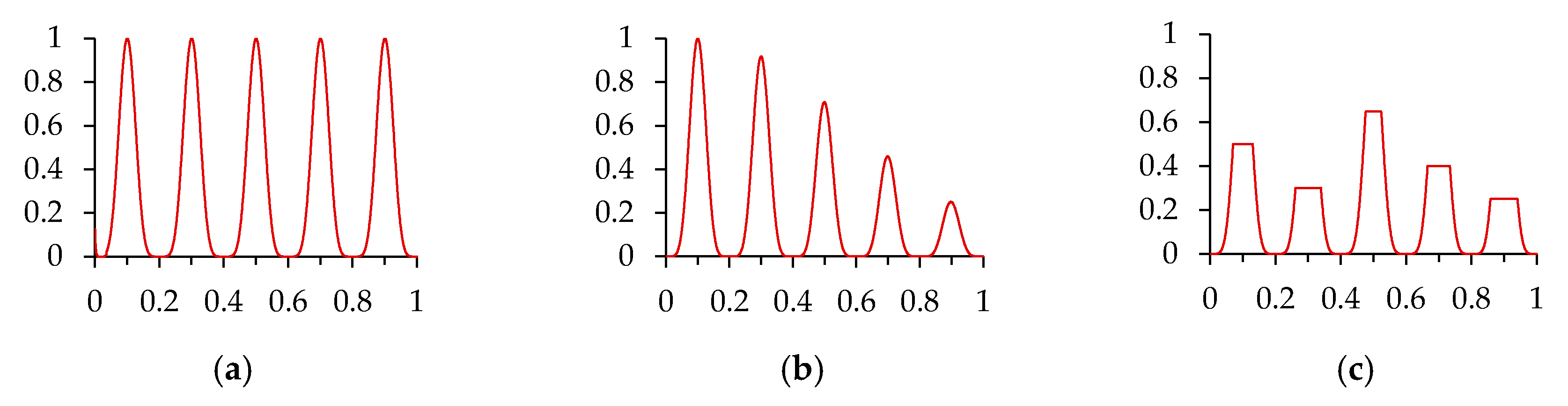
| 2 | F2(x) | Equal Maxima | 1 | x ∊ [0, 1] | 1.00 | 5 | 0 | |
| 3 | F3(x) | Uneven Decreasing Maxima | 1 | x ∊ [0, 1] | 1.00 | 1 | 4 | |
| 4 | F4(x, y) | Himmelblau | 2 | x, y ∊ [−6, 6] | 144.00 | 4 | 0 | |
| 5 | F5(x, y) | Six-Hump Camel Back | 2 | x ∊ [-1.9, 1.9]; y ∊ [−1.1, 1.1] | 8.36 | 2 | 5 | |
| 6 | F6() | Shubert | 2 | x1, x2 ∊ [−10, 10] | 18 | many | ||
| 7 | F7() | Vincent | 2 | x1, x2 ∊ [0.25, 10] | 95.06 | 36 | 0 | |
| 8 | F6() | Shubert | 3 | x1, x2, x3 ∊ [−10, 10] | 81 | many | ||
| 9 | F7() | Vincent | 3 | x1, x2, x3 ∊ [0.25, 10] | 926.86 | 216 | 0 | |
| 10 | F8() | Modified Rastrigin | 2 | x1, x2 ∊ [0, 1] | 1.00 | 12 | 0 | |
| 11 | F9() | Composition Function 1 | 2 | x1, x2 ∊ [−5, 5] | 6 | many | ||
| 12 | F10() | Composition Function 2 | 2 | x1, x2 ∊ [−5, 5] | 8 | many | ||
| 13 | F11() | Composition Function 3 | 2 | x1, x2 ∊ [−5, 5] | 6 | many | ||
| 14 | F11() | Composition Function 3 | 3 | x1, x2, x3 ∊ [−5, 5] | 6 | many | ||
| 15 | F12() | Composition Function 4 | 3 | x1, x2, x3 ∊ [-5, 5] | 8 | many | ||
| 16 | F11() | Composition Function 3 | 5 | x1, x2,…, x5 ∊ [-5, 5] | 6 | many | ||
| 17 | F12() | Composition Function 4 | 5 | x1, x2,…, x5 ∊ [-5, 5] | 8 | many | ||
| 18 | F11() | Composition Function 3 | 10 | x1, x2,…, x10 ∊ [-5, 5] | 6 | many | ||
| 19 | F12() | Composition Function 4 | 10 | x1, x2,…, x10 ∊ [-5, 5] | 8 | many | ||
| 20 | F12() | Composition Function 4 | 20 | x1, x2,…, x20 ∊ [-5, 5] | 8 | many |
| {Problem Ids} | {1, 2, 3, 4, 5, 10} | {1, 2, 3, 4, 5, 7, 9, 10} | {1 ~ 20} | |||
|---|---|---|---|---|---|---|
| NC-VMO | HVcMO20a | VMO-ASD | HVcMO20a | NVMO | HVcMO20a | |
| Mean PR | 0.696 | 1.000 | 0.523 | 0.994 | 0.698 | 0.885 |
| HVcMO20a vs. VMO-ASD | HVcMO20a vs. NVMO | ||||||||
|---|---|---|---|---|---|---|---|---|---|
| R+ | R− | W | Critical Value | H0 | R+ | R− | W | Critical Value | H0 |
| 21 | 0 | 0 | 0 | Rejected | 118 | 2 | 2 | 25 | Rejected |
| Mean | NEA2+ | RS-CMSA | SDE-Ga | ANBNWI-DE | HillVallEA18 | HillVallEA19 | HVcMO20a |
|---|---|---|---|---|---|---|---|
| PR | 0.807 | 0.856 | 0.833 | 0.855 | 0.885 | 0.890 | 0.885 |
| F1 | 0.855 | 0.911 | 0.884 | 0.887 | 0.930 | 0.933 | 0.930 |
| dynF1 | 0.806 | 0.829 | 0.376 | 0.727 | 0.869 | 0.883 | 0.876 |
| Scenario | p-Value | H0 |
|---|---|---|
| PR | Rejected | |
| F1 | Rejected | |
| dynF1 | Rejected |
| Volume of Search Space | Function Evaluations | Iterations (Failed Iterations) | Population Increase | |||
|---|---|---|---|---|---|---|
| HillVallEA19 | HVcMO20a | HillVallEA19 | HVcMO20a | HillVallEA19 | HVcMO20a | |
| medium | 114,080 | 116,480 | 19.11 (4.49) | 17.32 (3.70) | 684 | 401 |
| small + large | 51,805 | 53,751 | 6.84 (3.58) | 6.63 (3.38) | 723 | 593 |
| all sizes | 82,942 | 85,115 | 12.98 (4.03) | 11.98 (3.54) | 703 | 497 |
| Pop Size: 2^6 | Pop Size: 2^7 | Pop Size: 2^8 | Pop Size: 2^9 | Pop Size: 2^10 | All Pop Sizes | |||||||
|---|---|---|---|---|---|---|---|---|---|---|---|---|
| RoM | MoR | RoM | MoR | RoM | MoR | RoM | MoR | RoM | MoR | RoM | MoR | |
| Considering 50 Runs per Function for Every Population Size, Using a Tolerance of | ||||||||||||
| Max | 1.616 | 1.635 | 1.536 | 1.562 | 1.488 | 1.489 | 1.486 | 1.487 | 1.388 | 1.391 | 1.412 | 1.468 |
| Overall | 1.091 | 1.299 | 1.088 | 1.324 | 1.188 | 1.328 | 1.291 | 1.353 | 1.301 | 1.319 | 1.268 | 1.325 |
| Considering 250 Runs per Function: 50 Runs for Each Population Size, Using the 5 Levels of Tolerance | ||||||||||||
| Max | 1.609 | 1.626 | 1.498 | 1.523 | 1.495 | 1.503 | 1.464 | 1.465 | 1.407 | 1.409 | 1.424 | 1.457 |
| Overall | 1.065 | 1.305 | 1.297 | 1.314 | 1.345 | 1.352 | 1.334 | 1.337 | 1.314 | 1.335 | 1.273 | 1.329 |
| Using All Levels of Tolerance | ||||
|---|---|---|---|---|
| tratio | Runs Covered | % Covered | Runs Covered | % Covered |
| 1.00 | 327 | 6.54 | 1576 | 6.30 |
| 1.40 | 3714 | 74.28 | 18,293 | 73.17 |
| 1.65 | 4745 | 94.90 | 23,714 | 94.86 |
| 1.75 | 4852 | 97.04 | 24,231 | 96.92 |
| 2.00 | 4953 | 99.06 | 24,765 | 99.06 |
| 2.50 | 4993 | 99.86 | 24,982 | 99.93 |
| 4.00 | 5000 | 100.00 | 25,000 | 100.00 |
| Volume of Search Space | Final Pop Size | Total Population Size | Execution Time Units | ||||||||||||
|---|---|---|---|---|---|---|---|---|---|---|---|---|---|---|---|
| R+ | R− | W | Critical Value | H0 | R+ | R− | W | Critical Value | H0 | R+ | R− | W | Critical Value | H0 | |
| medium | 0 | 55 | 0 | 8 | Rejected | 0 | 55 | 0 | 8 | Rejected | 1 | 54 | 1 | 8 | Rejected |
| small + large | 1 | 27 | 1 | 2 | Rejected | 3 | 42 | 3 | 6 | Rejected | 47 | 8 | 8 | 8 | Rejected |
| all sizes | 1 | 152 | 1 | 35 | Rejected | 3 | 187 | 3 | 46 | Rejected | 85 | 125 | 85 | 52 | Accepted |
| Volumes of Medium Size | Volumes Small or Large | |||
|---|---|---|---|---|
| Mean | HillVallEA19 | HVcMO20a | HillVallEA19 | HVcMO20a |
| PR | 0.962 | 0.952 | 0.819 | 0.818 |
| F1 | 0.979 | 0.973 | 0.887 | 0.887 |
| dynF1 | 0.915 | 0.906 | 0.850 | 0.847 |
© 2020 by the authors. Licensee MDPI, Basel, Switzerland. This article is an open access article distributed under the terms and conditions of the Creative Commons Attribution (CC BY) license (http://creativecommons.org/licenses/by/4.0/).
Share and Cite
Navarro, R.; Kim, C.H. Niching Multimodal Landscapes Faster Yet Effectively: VMO and HillVallEA Benefit Together. Mathematics 2020, 8, 665. https://doi.org/10.3390/math8050665
Navarro R, Kim CH. Niching Multimodal Landscapes Faster Yet Effectively: VMO and HillVallEA Benefit Together. Mathematics. 2020; 8(5):665. https://doi.org/10.3390/math8050665
Chicago/Turabian StyleNavarro, Ricardo, and Chyon Hae Kim. 2020. "Niching Multimodal Landscapes Faster Yet Effectively: VMO and HillVallEA Benefit Together" Mathematics 8, no. 5: 665. https://doi.org/10.3390/math8050665
APA StyleNavarro, R., & Kim, C. H. (2020). Niching Multimodal Landscapes Faster Yet Effectively: VMO and HillVallEA Benefit Together. Mathematics, 8(5), 665. https://doi.org/10.3390/math8050665