A New Accelerated Viscosity Iterative Method for an Infinite Family of Nonexpansive Mappings with Applications to Image Restoration Problems

Abstract

The image restoration problem is one of the popular topics in image processing which is extensively studied by many authors because of its applications in various areas of science, engineering and medical image. The main aim of this paper is to introduce a new accelerated fixed algorithm using viscosity approximation technique with inertial effect for finding a common fixed point of an infinite family of nonexpansive mappings in a Hilbert space and prove a strong convergence result of the proposed method under some suitable control conditions. As an application, we apply our algorithm to solving image restoration problem and compare the efficiency of our algorithm with FISTA method which is a popular algorithm for image restoration. By numerical experiments, it is shown that our algorithm has more efficiency than that of FISTA.

1. Introduction

Let us first consider a simple linear inverse problem as the following form:

$$Ax=b+w,$$

(1)

where $x\in {\mathbb{R}}^{n\times 1}$ is the solution of the problem to be approximated, $A\in {\mathbb{R}}^{m\times n}$ and $b\in {\mathbb{R}}^{m\times 1}$ are known and $w\in {\mathbb{R}}^{m\times 1}$ is an additive noise vector. Such problems (1) arise in various applications such as the image and signal processing problems, astrophysical problems and data classification problems.

Further, one of their well-known applications is the problem of approximating the original image from the observed blurred and noisy image which is known as the image restoration problem. In this problem, $x,A$ and b represent the original image, blur operator and observed image, respectively.

The purpose of the image restoration problem is to minimize the additive noise in which the classical estimator is the least squares (LS) given as follows:

$$\widehat{x}:=\underset{x}{arg\; min}{\parallel Ax-b\parallel }_2^2,$$

(2)

where ${\parallel ·\parallel }_2$ is ${\ell }^2$-norm. However, this model still has some ill-conditions in the case that the least square solution has a huge norm which is thus meaningless. In 1977, Tikhonov and Arsenin [1] improved this ill-posed problem by introducing the regularization techniques which are known as the Tikhonov regularization (TR) model and it is of the following form:

$$\widehat{x}:=\underset{x}{arg\; min}{\{\parallel Ax-b\parallel }_2^2+{\lambda \parallel Lx\parallel }_2^2\},$$

(3)

for some regularization parameter $\lambda >0$ and Tikhonov matrix L.

On the other hand, another successful regularization method for improvement of Tikhonov regularization is known as the least absolute shrinkage and selection operator (LASSO) which was introduced by Tibshirani (1996). The method is to find a solution

$$\widehat{x}:=\underset{x}{arg\; min}{\{\parallel Ax-b\parallel }_2^2+{\lambda \parallel x\parallel }_1\},$$

(4)

where ${\parallel ·\parallel }_1$ is ${\ell }^1$-norm. The LASSO can be applied to regression problems and image restoration problems (see [2,3] for examples).

For solving (3) and (4), we extend them to a general naturally formulation, that is, the problem of finding the minimizer of sum of two functions:

$$\widehat{x}:=\underset{x}{arg\; min}\{h\left(x\right)+g\left(x\right)\}.$$

(5)

In order to solve (5), we assume the following:

• $h:{\mathbb{R}}^n\to \mathbb{R}$ is a smooth convex loss function and differentiable with L-Lipschitz continuous gradient, where $L>0$, i.e.,

  $$\parallel \nabla h\left(x\right)-\nabla h\left(y\right)\parallel \le L\parallel x-y\parallel ,\forall x,y\in {\mathbb{R}}^n;$$
• $g:{\mathbb{R}}^n\to \mathbb{R}\cup \{+\infty \}$ is a proper convex and lower semi-continuous function.

We here denote the set of all solutions of above problem by $arg\; min(h+g)$. It is well-known that the solution of (5) can be reformulated as the problem of finding a zero-solution $\widehat{x}$ such that

$$0\in \partial g\left(\widehat{x}\right)+\nabla h\left(\widehat{x}\right),$$

(6)

where $\partial g$ is the subdifferential of function g and $\nabla h$ is the gradient operator of function h (see [4] for more details). Moreover, the problem (6) can be solved by using the proximal gradient technique which was presented by Parikh and Boyd [5], i.e., if $\widehat{x}$ is a solution of (6), then it is a fixed point of a forward-backward operator T defined by $T:={\mathrm{prox}}_{\lambda g}(I-\lambda \nabla h)$ for $\lambda >0$. The operator ${\mathrm{prox}}_{\lambda g}$ is called the proximity operator with respect to $\lambda$ and function g. We know that T is a nonexpansive mapping whenever $\lambda \in \left(0,\frac{2}{L}\right)$. It is easily seen that ${\mathrm{prox}}_{\lambda g}$ is an example of the resolvent of $\partial g$, that is, ${\mathrm{prox}}_{\lambda g}=J_{\lambda }^{\partial g}={(I+\lambda \partial g)}^{-1}$, see Section 2 for more details.

We have seen from above fact that fixed point theory plays very important role in solving and developing of the image and signal processing problems which can be applied to solving many real-world problems in digital image processing such as medical image and astronomy as well as image processing for security sections. Fixed point theory focuses on two important problems. The first one is an existence problem of a solution of many kind of real-world problems while the other problem is a problem of how to approximate such solutions of the interested problems. For the past two decades, a lot of fixed point iteration processes were introduced and studied to solving many practical problems. It is well-known by Banach Contraction Principle that every contraction map from a complete metric space X into itself has a unique fixed point.

A mapping T from a metric space $(X,d)$ into itself is called a contraction if there is a $k\in [0,1)$ such that $d(Tx,Ty)\le kd(x,y)$ for all $x,y\in X$.

It is well-known that the Picard iteration process, defined by $x_1\in X$ and

$$x_{n+1}=T{x}_n,\forall n\ge 1,$$

converges to a unique fixed point $x^{\ast }$ of T.

It is observed that when $k=1$ in above inequality, we have a new nonlinear mapping, called nonexpansive mapping. This type of mapping plays a crucial role to solving many optimization problems and economics.

From now on, we would like to provide some background concerning various iteration methods for finding a fixed point of nonexpansive and other nonlinear mappings.

Mann [6] was the first who introduced a modified iterative method known as Mann iteration process in Hilbert space H as follows: $x_1\in H$,

$$x_{n+1}={\alpha }_n{x}_n+(1-{\alpha }_n)T{x}_n,\forall n\ge 1,$$

where $\left\{{\alpha }_n\right\}$ is a real sequence in $[0,1]$. In 1974, Ishikawa extended Mann iteration, called the Ishikawa iteration process, by the following method: For an initial point $x_1$,

$$\left\{\begin{array}{cc}\hfill y_n& =(1-{\alpha }_n)x_n+{\alpha }_{n}T{x}_n,\hfill \\ \hfill x_{n+1}& =(1-{\beta }_n)x_n+{\beta }_{n}T{y}_n,\forall n\ge 1,\hfill \end{array}\right.$$

(7)

where $\left\{{\alpha }_n\right\}$, $\left\{{\beta }_n\right\}\subset [0,1]$. Agarwal et al. employed the idea of the Ishikawa method to introduce S-iteration process as follows: For an initial point $x_1$,

$$\left\{\begin{array}{cc}\hfill y_n& =(1-{\alpha }_n)x_n+{\alpha }_{n}T{x}_n,\hfill \\ \hfill x_{n+1}& =(1-{\beta }_n)T{x}_n+{\beta }_{n}T{y}_n,\forall n\ge 1,\hfill \end{array}\right.$$

(8)

where $\left\{{\alpha }_n\right\}$ and $\left\{{\beta }_n\right\}$ are sequences in $[0,1]$. They showed that the convergence behavior of S-iteration is better than that of Mann and of Ishikawa iterations.

Because Mann iteration obtained only weak convergence (see [7] for more details). In 2000, Moufafi [8] introduced a well-known viscosity approximation was defined as follows: For $x_1\in H$,

$$x_{n+1}={\alpha }_{n}f\left(x_n\right)+(1-{\alpha }_n)T{x}_n,\forall n\ge 1,$$

(9)

where $\left\{{\alpha }_n\right\}\subset [0,1]$ and f is a contraction mapping. Under some suitable control conditions, he proved that $\left\{x_n\right\}$ converges strongly to a fixed point of T, when T is a nonexpansive mapping. Recently, authors in [9] proposed the viscosity-based inertial forward-backward algorithm (VIFBA), for solving (5) by finding a common fixed point of an infinite family $\left\{T_n\right\}$ of forward-backward operators. For initial points $x_0,x_1\in H$, they define their method as follows:

$$\left\{\begin{array}{cc}\hfill y_n& =x_n+{\theta }_n(x_n-x_{n-1}),\hfill \\ \hfill z_n& =(1-{\beta }_n)y_n+{\beta }_{n}f\left(y_n\right),\hfill \\ \hfill x_{n+1}& =T_n{z}_n,\forall n\ge 1,\hfill \end{array}\right.$$

(10)

where f is a contraction mapping on H and $\left\{{\alpha }_n\right\},\left\{{\beta }_n\right\}$ are sequences in $[0,1]$. Here, the inertial term is represented by the term ${\theta }_n(x_n-x_{n-1})$ which was firstly introduced by Nesterov [10]. This algorithm is also applied to solve the regression and recognition problems.

In 2009, Beck and Teboulle introduced a fast iterative shrinkage-thresholding algorithm (FISTA) which was defined by

$$\left\{\begin{array}{cc}\hfill y_n& =T{x}_n,\hfill \\ \hfill t_{n+1}& =\frac{1+\sqrt{1+4t_n^2}}{2},\hfill \\ \hfill {\theta }_n& =\frac{t_n-1}{t_{n+1}},\hfill \\ \hfill x_{n+1}& =y_n+{\theta }_n(y_n-y_{n-1}),\forall n\ge 1,\hfill \end{array}\right.$$

(11)

where $T={\mathrm{prox}}_{\lambda g}(I-\lambda \nabla h)$ for $\lambda >0$ and the initial points $x_1=y_0\in {\mathbb{R}}^n$ and $t_1=1$. Moreover, they applied their algorithm to the image restoration problems (see [3] for more details). It is pointed out from this work that the LASSO model is a suitable model for image restoration problems.

Motivated and inspired by all of these researches going on in this direction, in this paper, we introduce a new accelerated algorithm for finding a common fixed point of a family of nonexpansive mappings $\left\{T_n\right\}$ in Hilbert spaces based on the concept of inertial forward-backward, of Mann and of viscosity algorithms. Then a strong convergence theorem is established under some control conditions. Moreover, we apply the main results to solving image restoration problems and compare efficiency of our proposed algorithm with others. The presented results in this work also improve some well-known results in the literature.

This paper is organized as follows: In Section 2, Preliminaries, we recall some definitions and the useful facts which will be used in the later sections. We prove and analyze a strong convergence of the proposed algorithm in Section 3, Main Results. In the next section, Section 4 (Applications), we apply our main result to solving image restoration problems. Finally, the last section, Section 5 (Conclusions), is the summary of our work.

2. Preliminaries

Throughout this paper, we let H be a real Hilbert space with inner product $\langle ·,·\rangle$ and norm $\parallel ·\parallel$. Let $\left\{x_n\right\}$ be a sequence in H. We use $x_n\to x$ stands for $\left\{x_n\right\}$ converges strongly to x and $x_n\rightharpoonup x$ stands for $\left\{x_n\right\}$ converges weakly to x. Let $T:C\to C$ be a mapping from a nonempty closed convex subset of H into itself. A fixed point of T is a point $x\in C$ such that $x=Tx$. The set of all fixed points of T is denoted by $F\left(T\right)$, that is,

$$F\left(T\right):=\{x\in C:x=Tx\}.$$

A mapping $T:C\to H$ is said to be L-Lipschitzian, if there exists a constant $L>0$ such that

$$\parallel Tx-Ty\parallel \le L\parallel x-y\parallel ,\forall x,y\in C.$$

If $L=1$, then T is said to be a nonexpansive mapping. It is well-known that if T is nonexpansive, then $F\left(T\right)$ is closed and convex.

We call a mapping $f:C\to H$ a contraction, if there exists a constant $k\in [0,1)$ such that

$$\parallel f\left(x\right)-f\left(y\right)\parallel \le k\parallel x-y\parallel ,\forall x,y\in C.$$

Here, we say that f is a k-contraction mapping.

Let $A:H\to 2^H$. The domain of A is the set $D\left(A\right):=\{x\in H:Ax\ne \varnothing \}$ and the range of A is the set $R\left(A\right):=\bigcup \{Az:z\in D(A\left)\right\}$. The inverse of A is denoted by $A^{-1}$ is defined as follows: $x\in A^{-1}y$ if and only if $y\in Ax$. The graph of A is denoted by $G\left(A\right)$ and $G\left(A\right):=\left\{\right(x,u):u\in Ax\}$.

An operator $A:H\to 2^H$ is said to be monotone if $\langle u-v,x-y\rangle \ge 0,\mathrm{for}\mathrm{all}u\in Ax\mathrm{and}v\in Ay.$ A monotone operator A on H is said to be maximal if the graph of A is not properly contained in any graph of other monotone operators on H. It is well-known that A is maximal if and only if for $x\in D\left(A\right)$ and $u\in Ax$, $\langle u-v,x-y\rangle \ge 0\mathrm{implies}(y,v)\in G\left(A\right).$

Moreover, A is a maximally monotone operator if and only if $R(I+\lambda A)=H$ for every $\lambda >0$, where I is an identity operator. We also know that the subdifferential of a proper lower semicontinuous convex function is a nice example of a maximal monotone.

For a function $g:H\to [-\infty ,+\infty ]$. The subdifferential $\partial g:H\to 2^H$ of g at $x\in H$, with $g\left(x\right)\in \mathbb{R}$, is the set $\partial g\left(x\right):=\{x^{\ast }\in H:g\left(x\right)+\langle y-x,x^{\ast }\rangle \le g\left(y\right),\forall y\in H\}$. We take by convention $\partial g\left(x\right):=\varnothing$, if $g\left(x\right)\in \{\pm \infty \}$. If $g\in {\mathsf{\Gamma }}_0\left(H\right)$, the set of proper lower semicontinuous convex functions from H to $(-\infty ,+\infty ]$, then $\partial g$ is maximally monotone (see [11] for more details).

For a maximally monotone operator A and $\lambda >0$, the resolvent of A for $\lambda$ is defined to be a single-valued operator $J_{\lambda }^A:R(I+\lambda A)\to D\left(A\right)$, where $J_{\lambda }^A={(I+\lambda A)}^{-1}$. It is well-known that $J_{\lambda }^A$ is a nonexpansive mapping and $F\left(J_{\lambda }^A\right)=A^{-1}0$, where $A^{-1}0:=\{x\in H:0\in Ax\}$ and it is called the set of all zero (or null) points of A.

Let $A:H\to 2^H$ be a multi-valued mapping and $B:H\to H$ a single-valued nonlinear mapping. The quasi-variational inclusion problem is the problem of finding a point $x\in H$ such that

$$\begin{array}{c}\hfill 0\in Ax+Bx.\end{array}$$

(12)

The set of all solutions of the problem (12) is denoted by ${(A+B)}^{-1}0.$

A classical method for solving the problem (12) is the forward-backward method [12,13,14] which was first introduced by Combettes and Hirstoaga [15] in the following manner: $x_1\in H$ and

$$\begin{array}{c}\hfill x_{n+1}=J_{\lambda }^A(x_n-\lambda B{x}_n),\forall n\ge 1,\end{array}$$

(13)

where $\lambda >0$. Moreover, we have from [16], if A is a maximally monotone operator and B is an L-Lipschitz continuous, then $F\left(J_{\lambda }^A(I-\lambda B)\right)={(A+B)}^{-1}0.$

Definition 1.

Let$g\in {\mathsf{\Gamma }}_0\left(H\right)$and$\lambda >0$. The proximity operator of parameter λ of g at$x\in H$is denoted by${prox}_{\lambda g}$and it is defined by

$${prox}_{\lambda g}x:=\underset{y\in H}{arg\; min}\left\{g\left(y\right)+\frac{1}{2\lambda }{\parallel y-x\parallel }^2\right\}.$$

It is well-known that if $g\in {\mathsf{\Gamma }}_0\left(H\right)$, then $J_{\lambda }^{\partial g}={\mathrm{prox}}_{\lambda g}$, that is, the proximity operator is an example of resolvent operator. Moreover, if $g={\parallel ·\parallel }_1$, then

$${\mathrm{prox}}_{{\lambda \parallel ·\parallel }_1}x={\mathrm{sign}\left(x\right)max\{\parallel x\parallel }_1-\lambda ,0\},$$

where sign is a signum function (see  [4] for more details).

The following basic definitions and well-known results are also needed for proving our main results.

Lemma 1. 

([17,18]) Let H be a real Hilbert space. For$x,y\in H$and any arbitrary real number λ in$[0,1]$, the following hold:

1.

${\parallel x\pm y\parallel }^2={\parallel x\parallel }^2\pm 2\langle x,y\rangle +{\parallel y\parallel }^2$;

2.

${\parallel x+y\parallel }^2\le {\parallel x\parallel }^2+2\langle y,x+y\rangle$;

3.

${\parallel \lambda x+(1-\lambda )y\parallel }^2={\lambda \parallel x\parallel }^2+{(1-\lambda )\parallel y\parallel }^2-\lambda (1-\lambda ){\parallel x-y\parallel }^2$.

The identity in Lemma 1(3) implies that the following equality holds:

$$\begin{array}{c}\hfill {\parallel \alpha x+\beta y+\gamma z\parallel }^2={\alpha \parallel x\parallel }^2+{\beta \parallel y\parallel }^2+{\gamma \parallel z\parallel }^2{-\alpha \beta \parallel x-y\parallel }^2{-\beta \gamma \parallel y-z\parallel }^2-\alpha \gamma {\parallel x-z\parallel }^2,\end{array}$$

(14)

for all $x,y,z\in H$ and $\alpha ,\beta ,\gamma \in [0,1]$ with $\alpha +\beta +\gamma =1$.

Let C be a nonempty closed convex subset of a Hilbert space H. We know that for each element $x\in H$, there exists a unique point in C, say $P_{C}x$, such that

$$\parallel x-P_{C}x\parallel \le \parallel x-y\parallel ,\forall y\in C.$$

Such a mapping $P_C$ is called the metric projection of H onto C. It is well-known that $P_C$ is a nonexpansive mapping. Moreover, $P_C$ can be characterized by the following inequality

$$\langle x-P_{C}x,y-P_{C}x\rangle \le 0$$

(15)

holds for all $x\in H$ and $y\in C$ (see [19] for more details).

We next recall the following properties which are useful for proving our main result, we refer to [20,21].

Let $\left\{T_n\right\}$ and $\mathcal{T}$ be families of nonexpansive mappings of H into itself such that $\varnothing \ne F\left(\mathcal{T}\right)\subset {\bigcap }_{n=1}^{\infty }F\left(T_n\right)$, where $F\left(\mathcal{T}\right)$ is the set of all common fixed points of $\mathcal{T}$. We say that $\left\{T_n\right\}$ satisfies NST-condition(I) with $\mathcal{T}$ if for each bounded sequence $\left\{x_n\right\}$ such that ${lim}_{n\to \infty }\parallel x_n-T_n{x}_n\parallel =0$, it follows

$$\underset{n\to \infty }{lim}\parallel x_n-T{x}_n\parallel =0\mathrm{for}\mathrm{all}T\in \mathcal{T}.$$

In particular, if $\mathcal{T}$ consists of one mapping T, i.e., $\mathcal{T}=\left\{T\right\}$, then $\left\{T_n\right\}$ is said to satisfy NST-condition(I) with T.

Lemma 2.

Let$\left\{T_n\right\}$be a family of nonexpansive mappings of H into itself and$T:H\to H$a nonexpansive mapping with$\varnothing \ne F\left(T\right)\subset {\bigcap }_{n=1}^{\infty }F\left(T_n\right)$. One always has, if$\left\{T_n\right\}$satisfies NST-condition(I) with T, then$\left\{T_t\right\}$also satisfies NST-condition(I) with T, for any subsequences$\left\{t\right\}$of positive integers.

Proof. 

Let $\left\{x_t\right\}$ be a bounded sequence such that $\parallel x_t-T_t{x}_t\parallel \to 0$ as $t\to +\infty$. Take $u\in F\left(T\right)$. Define the sequence $\left\{x_n\right\}$ by

$$x_n:=\left\{\begin{array}{cc}{x}_t\hfill & \mathrm{if}n=t;\hfill \\ u\hfill & \mathrm{otherwise}.\hfill \end{array}\right.$$

Then $\left\{x_n\right\}$ is bounded. Moreover, we have that

$$\underset{n\to \infty }{lim}\parallel x_n-T_n{x}_n\parallel =\underset{t\to \infty }{lim}\parallel x_t-T_t{x}_t\parallel =0,$$

due to u is a fixed point of $T_n$ for all $n\in \mathbb{N}$. By the NST-condition(I) with T on $\left\{T_n\right\}$, we obtain that

$$\underset{t\to \infty }{lim}\parallel x_t-T{x}_t\parallel =\underset{n\to \infty }{lim}\parallel x_n-T{x}_n\parallel =0.$$

Thus, $\left\{T_t\right\}$ satisfies NST-condition(I) with T. ☐

Proposition 1. 

([22]) Let H be a Hilbert space. Let$A:H\to 2^H$be a maximally monotone operator and$B:H\to H$an L-Lipschitz operator, where$L>0$. Let$T_n=J_{{\lambda }_n}^A(I-{\lambda }_{n}B)$, where$0<{\lambda }_n<\frac{2}{L}$for all$n\ge 1$and let$T=J_{\lambda }^A(I-\lambda B)$, where$0<\lambda <\frac{2}{L}$with${\lambda }_n\to \lambda$. Then$\left\{T_n\right\}$satisfies the NST-condition(I) with T.

The following lemmas are crucial for proving our main results.

Lemma 3. 

([23]) Let H be a real Hilbert space and$T:H\to H$a nonexpansive mapping with$F\left(T\right)\ne \varnothing$. Then the mapping$I-T$is demiclosed at zero, i.e., for any sequences$\left\{x_n\right\}$in H such that$x_n\rightharpoonup x\in H$and$\parallel x_n-T{x}_n\parallel \to 0$imply$x\in F\left(T\right)$.

Lemma 4. 

([24,25]) Let$\left\{s_n\right\}$,$\{{\xi }_n\}$be sequences of nonnegative real numbers,$\left\{{\delta }_n\right\}$a sequence in [0,1] and$\left\{t_n\right\}$a sequence of real numbers such that

$$s_{n+1}\le (1-{\delta }_n)s_n+{\delta }_n{t}_n+{\xi }_n,$$

for all$n\in \mathbb{N}.$If the following conditions hold:

1. 

${\sum }_{n=1}^{\infty }{\delta }_n=\infty$;

2. 

${\sum }_{n=1}^{\infty }{\xi }_n<\infty$;

2. 

${lim\; sup}_{n\to \infty }{t}_n\le 0$.

Then${lim}_{n\to \infty }{s}_n=0$.

Lemma 5. 

([26]) Let$\left\{{\mathsf{\Theta }}_n\right\}$be a sequence of real numbers that does not decrease at infinity in the sense that there exists a subsequence$\{{\mathsf{\Theta }}_{n_i}\}$of$\left\{{\mathsf{\Theta }}_n\right\}$which satisfies${\mathsf{\Theta }}_{n_i}<{\mathsf{\Theta }}_{n_i+1}$for all$i\in \mathbb{N}$. Define the sequence${\left\{\tau \left(n\right)\right\}}_{n\ge n_0}$of integers as follows:

$$\tau \left(n\right):=max\{k\le n:{\mathsf{\Theta }}_k<{\mathsf{\Theta }}_{k+1}\},$$

where$n_0\in \mathbb{N}$such that$\{k\le n_0:{\mathsf{\Theta }}_k<{\mathsf{\Theta }}_{k+1}\}\ne \varnothing$. Then the following hold:

1. 

$\tau \left(n_0\right)\le \tau (n_0+1)\le \dots$and$\tau \left(n\right)\to \infty$;

2. 

${\mathsf{\Theta }}_{\tau \left(n\right)}\le {\mathsf{\Theta }}_{\tau \left(n\right)+1}$and${\mathsf{\Theta }}_n\le {\mathsf{\Theta }}_{\tau \left(n\right)+1}$for all$n\ge n_0$.

3. Main Results

In this section, we first give a new algorithm for finding a common fixed point of a family of nonexpansive mappings in a real Hilbert space. We then prove its strong convergence under some suitable conditions.

We now propose a new accelerated algorithm for approximating a solution of our common fixed point problem as the following.

Let H be a real Hilbert space. Let $\left\{T_n\right\}$ be a family of nonexpansive mappings on H into itself. Let f be a k-contraction mapping on H with $k\in (0,1)$ and let $\{{\eta }_n\}\subset (0,\infty )$ and $\left\{{\sigma }_n\right\},\left\{{\alpha }_n\right\},\{{\beta }_n\},\{{\gamma }_n\}\subset (0,1)$.

We next prove the convergence of the sequence generated by Algorithm 1. To this end, we assume that the algorithm does not stop after finitely many iterations.

Algorithm 1: NAVA (New Accelerated Viscosity Algorithm).

Initialization: Take $x_0,x_1\in H$. Choose $\theta \ge 0$.     For $n\ge 1$:         Set $${\theta }_n:=\left\{\begin{array}{cc}{\displaystyle min\left\{\theta ,\frac{{\eta }_n{\alpha }_n}{\parallel x_n-x_{n-1}\parallel }\right\}}\hfill & \mathrm{if}{x}_n\ne x_{n-1};\hfill \\ \theta \hfill & \mathrm{otherwise}.\hfill \end{array}\right.$$         Compute $$\begin{array}{cc}\hfill y_n& :=x_n+{\theta }_n(x_n-x_{n-1}),\hfill \\ \hfill z_n& :=(1-{\sigma }_n)y_n+{\sigma }_n{T}_n{y}_n,\hfill \\ \hfill x_{n+1}& :={\alpha }_{n}f\left(x_n\right)+{\beta }_n{T}_n{y}_n+{\gamma }_n{T}_n{z}_n.\hfill \end{array}$$

Theorem 1.

Let$\left\{T_n\right\}$be a family of nonexpansive mappings and$T:H\to H$a nonexpansive mapping such that$\varnothing \ne F\left(T\right)\subset {\bigcap }_{n=1}^{\infty }F\left(T_n\right)$. Suppose that$\left\{T_n\right\}$satisfies NST-condition(I) with T. Let$\left\{x_n\right\}$be the sequence generated by Algorithm 1 such that the following additional conditions hold:

1.

${\alpha }_n+{\beta }_n+{\gamma }_n=1$;

2.

$0<a\le {\sigma }_n\le a^{\prime }<1$;

3.

$0<b\le {\beta }_n\le b^{\prime }<1$;

4.

$0<c\le {\gamma }_n\le c^{\prime }<1$;

5.

${lim}_{n\to \infty }{\eta }_n=0$;

6.

${lim}_{n\to \infty }{\alpha }_n=0$and${\sum }_{n=1}^{\infty }{\alpha }_n=\infty$,

for some positive real numbers$a,b,c,a^{\prime },b^{\prime },c^{\prime }$. Then the sequence$\left\{x_n\right\}$converges strongly to$u\in F\left(T\right)$, where$u=P_{F\left(T\right)}f\left(u\right)$.

Proof. 

Let $u\in F\left(T\right)$ be such that $u=P_{F\left(T\right)}f\left(u\right)$. First of all, we show that $\left\{x_n\right\}$ is bounded. By the definition of $y_n$ and of $z_n$, we have

$$\begin{array}{cc}\hfill \parallel y_n-u\parallel & =\parallel x_n+{\theta }_n(x_n-x_{n-1})-u\parallel \hfill \\ \hfill & \le \parallel x_n-u\parallel +{\theta }_n\parallel x_n-x_{n-1}\parallel ,\forall n\ge 1,\hfill \end{array}$$

(16)

and

$$\begin{array}{cc}\hfill \parallel z_n-u\parallel & =\parallel (1-{\sigma }_n)y_n+{\sigma }_n{T}_n{y}_n-u\parallel \hfill \\ \hfill & \le (1-{\sigma }_n)\parallel y_n-u\parallel +{\sigma }_n\parallel T_n{y}_n-u\parallel \hfill \\ \hfill & =(1-{\sigma }_n)\parallel y_n-u\parallel +{\sigma }_n\parallel T_n{y}_n-T_{n}u\parallel \hfill \\ \hfill & \le (1-{\sigma }_n)\parallel y_n-u\parallel +{\sigma }_n\parallel y_n-u\parallel \hfill \\ \hfill & =\parallel y_n-u\parallel ,\forall n\ge 1.\hfill \end{array}$$

(17)

From (16) and (17), we also have that

$$\begin{array}{cc}\hfill \parallel x_{n+1}-u\parallel & =\parallel {\alpha }_{n}f\left(x_n\right)+{\beta }_n{T}_n{y}_n+{\gamma }_n{T}_n{z}_n-u\parallel \hfill \\ \hfill & =\parallel {\alpha }_n(f\left(x_n\right)-u)+{\beta }_n(T_n{y}_n-u)+{\gamma }_n(T_n{z}_n-u)\parallel \hfill \\ \hfill & \le {\alpha }_n\parallel f\left(x_n\right)-u\parallel +{\beta }_n\parallel T_n{y}_n-u\parallel +{\gamma }_n\parallel T_n{z}_n-u\parallel \hfill \\ \hfill & ={\alpha }_n\parallel f\left(x_n\right)-u\parallel +{\beta }_n\parallel T_n{y}_n-T_{n}u\parallel +{\gamma }_n\parallel T_n{z}_n-T_{n}u\parallel \hfill \\ \hfill & \le {\alpha }_n\parallel f\left(x_n\right)-f\left(u\right)\parallel +{\alpha }_n\parallel f\left(u\right)-u\parallel +{\beta }_n\parallel y_n-u\parallel +{\gamma }_n\parallel z_n-u\parallel \hfill \\ \hfill & \le {\alpha }_{n}k\parallel x_n-u\parallel +{\alpha }_n\parallel f\left(u\right)-u\parallel +({\beta }_n+{\gamma }_n)\parallel y_n-u\parallel \hfill \\ \hfill & \le {\alpha }_{n}k\parallel x_n-u\parallel +{\alpha }_n\parallel f\left(u\right)-u\parallel +({\beta }_n+{\gamma }_n)(\parallel x_n-u\parallel +{\theta }_n\parallel x_n-x_{n-1}\parallel )\hfill \\ \hfill & \le ({\alpha }_{n}k+{\beta }_n+{\gamma }_n)\parallel x_n-u\parallel +{\alpha }_n\parallel f\left(u\right)-u\parallel +({\beta }_n+{\gamma }_n){\theta }_n\parallel x_n-x_{n-1}\parallel \hfill \\ \hfill & \le ({\alpha }_{n}k+{\beta }_n+{\gamma }_n)\parallel x_n-u\parallel +{\alpha }_n\parallel f\left(u\right)-u\parallel +(b^{\prime }+c^{\prime }){\theta }_n\parallel x_n-x_{n-1}\parallel \hfill \\ \hfill & =(1-{\alpha }_n(1-k))\parallel x_n-u\parallel +{\alpha }_n\parallel f\left(u\right)-u\parallel \hfill \\ \hfill & +(b^{\prime }+c^{\prime }){\alpha }_n·\frac{{\theta }_n}{{\alpha }_n}\parallel x_n-x_{n-1}\parallel ,\forall n\ge 1.\hfill \end{array}$$

(18)

According to the definition of ${\theta }_n$ and the assumption (5), we have

$$\frac{{\theta }_n}{{\alpha }_n}\parallel x_n-x_{n-1}\parallel \to 0\mathrm{as}n\to \infty .$$

Then there exists a positive constant $M_1>0$ such that

$$\frac{{\theta }_n}{{\alpha }_n}\parallel x_n-x_{n-1}\parallel \le M_1,\forall n\ge 1.$$

From (18), we obtain

$$\begin{array}{cc}\hfill \parallel x_{n+1}-u\parallel & \le (1-{\alpha }_n(1-k))\parallel x_n-u\parallel +{\alpha }_n\parallel f\left(u\right)-u\parallel +{\alpha }_n(b^{\prime }+c^{\prime })M_1\hfill \\ \hfill & =(1-{\alpha }_n(1-k))\parallel x_n-u\parallel +{\alpha }_n(\parallel f\left(u\right)-u\parallel +(b^{\prime }+c^{\prime })M_1)\hfill \\ \hfill & =(1-{\alpha }_n(1-k))\parallel x_n-u\parallel +{\alpha }_n(1-k)\left[\frac{\parallel f\left(u\right)-u\parallel +(b^{\prime }+c^{\prime })M_1}{1-k}\right]\hfill \\ \hfill & \le max\left\{\parallel x_n-u\parallel ,\frac{\parallel f\left(u\right)-u\parallel +(b^{\prime }+c^{\prime })M_1}{1-k}\right\}\hfill \\ \hfill & ⋮\hfill \\ \hfill & \le max\left\{\parallel x_1-u\parallel ,\frac{\parallel f\left(u\right)-u\parallel +(b^{\prime }+c^{\prime })M_1}{1-k}\right\},\forall n\ge 1.\hfill \end{array}$$

This implies $\left\{x_n\right\}$ is bounded and so are $\{y_n\},\left\{z_n\right\},\left\{f\left(x_n\right)\right\}$ and $\{T_n{y}_n\}$.

Indeed, we have that for all $n\ge 1$,

$$\begin{array}{cc}\hfill {\parallel y_n-u\parallel }^2& =\parallel x_n+{\theta }_n(x_n-x_{n-1}){-u\parallel }^2\hfill \\ \hfill & =\parallel (x_n-u)+{\theta }_n(x_n-x_{n-1}){\parallel }^2\hfill \\ \hfill & \le \parallel x_n{-u\parallel }^2+2{\theta }_n\parallel x_n-u\parallel \parallel x_n-x_{n-1}\parallel +{\theta }_n^2{\parallel x_n-x_{n-1}\parallel }^2.\hfill \end{array}$$

(19)

By Lemma 1(2), (14) and (17) we have

$$\begin{array}{cc}\hfill {\parallel x_{n+1}-u\parallel }^2& =\parallel {\alpha }_{n}f\left(x_n\right)+{\beta }_n{T}_n{y}_n+{\gamma }_n{T}_n{z}_n{-u\parallel }^2\hfill \\ & =\parallel {\alpha }_n(f\left(x_n\right)-f\left(u\right))+{\beta }_n(T_n{y}_n-u)+{\gamma }_n(T_n{z}_n-u)+{\alpha }_n(f\left(u\right)-u){\parallel }^2\hfill \\ & \le \parallel {\alpha }_n(f\left(x_n\right)-f\left(u\right))+{\beta }_n(T_n{y}_n-u)+{\gamma }_n(T_n{z}_n-u){\parallel }^2+2{\alpha }_n\langle f\left(u\right)-u,x_{n+1}-u\rangle \hfill \\ & \le {\alpha }_n\parallel f\left(x_n\right)-f\left(u\right){\parallel }^2+{\beta }_n{\parallel T_n{y}_n-u\parallel }^2+{\gamma }_n{\parallel T_n{z}_n-u\parallel }^2+2{\alpha }_n\langle f\left(u\right)-u,x_{n+1}-u\rangle \hfill \\ & ={\alpha }_n\parallel f\left(x_n\right)-f\left(u\right){\parallel }^2+{\beta }_n{\parallel T_n{y}_n-T_{n}u\parallel }^2+{\gamma }_n{\parallel T_n{z}_n-T_{n}u\parallel }^2+2{\alpha }_n\langle f\left(u\right)-u,x_{n+1}-u\rangle \hfill \\ & \le {\alpha }_n{k}^2{\parallel x_n-u\parallel }^2+{\beta }_n{\parallel y_n-u\parallel }^2+{\gamma }_n{\parallel z_n-u\parallel }^2+2{\alpha }_n\langle f\left(u\right)-u,x_{n+1}-u\rangle \hfill \\ & \le {\alpha }_n{k}^2{\parallel x_n-u\parallel }^2+({\beta }_n+{\gamma }_n){\parallel y_n-u\parallel }^2+2{\alpha }_n\langle f\left(u\right)-u,x_{n+1}-u\rangle ,\forall n\ge 1\hfill \end{array}$$

(20)

It follows from (19) with $0<k<1$ that

$$\begin{array}{cc}\hfill {\parallel x_{n+1}-u\parallel }^2& \le {\alpha }_{n}k{\parallel x_n-u\parallel }^2\hfill \\ \hfill & +({\beta }_n+{\gamma }_n)({\parallel x_n-u\parallel }^2+2{\theta }_n\parallel x_n-u\parallel \parallel x_n-x_{n-1}\parallel +{\theta }_n^2{\parallel x_n-x_{n-1}\parallel }^2)\hfill \\ \hfill & +2{\alpha }_n\langle f\left(u\right)-u,x_{n+1}-u\rangle \hfill \\ \hfill & =(1-{\alpha }_n(1-k)){\parallel x_n-u\parallel }^2\hfill \\ \hfill & +({\beta }_n+{\gamma }_n){\theta }_n\parallel x_n-x_{n-1}\parallel \left(2\parallel x_n-u\parallel +{\theta }_n\parallel x_n-x_{n-1}\parallel \right)\hfill \\ \hfill & +2{\alpha }_n\langle f\left(u\right)-u,x_{n+1}-u\rangle ,\forall n\ge 1.\hfill \end{array}$$

(21)

Since

$${\theta }_n\parallel x_n-x_{n-1}\parallel ={\alpha }_n·\frac{{\theta }_n}{{\alpha }_n}\parallel x_n-x_{n-1}\parallel \to 0,\mathrm{as}n\to \infty ,$$

there exists a positive constant $M_2>0$ such that

$${\theta }_n\parallel x_n-x_{n-1}\parallel \le M_2,\forall n\ge 1.$$

From the inequality (21), we derive that for all $n\ge 1$,

$$\begin{array}{cc}\hfill {\parallel x_{n+1}-u\parallel }^2& \le (1-{\alpha }_n(1-k)){\parallel x_n-u\parallel }^2+3M_3({\beta }_n+{\gamma }_n){\theta }_n\parallel x_n-x_{n-1}\parallel +2{\alpha }_n\langle f\left(u\right)-u,x_{n+1}-u\rangle \hfill \\ & \le (1-{\alpha }_n(1-k)){\parallel x_n-u\parallel }^2+3M_3(b^{\prime }+c^{\prime }){\theta }_n\parallel x_n-x_{n-1}\parallel +2{\alpha }_n\langle f\left(u\right)-u,x_{n+1}-u\rangle \hfill \\ & \le (1-{\alpha }_n(1-k)){\parallel x_n-u\parallel }^2\hfill \\ & +{\alpha }_n(1-k)\left[\frac{3M_3(b^{\prime }+c^{\prime })}{1-k}·\frac{{\theta }_n}{{\alpha }_n}\parallel x_n-x_{n-1}\parallel +\frac{2}{1-k}\langle f\left(u\right)-u,x_{n+1}-u\rangle \right],\hfill \end{array}$$

(22)

where $M_3:={sup}_{n\ge 1}\{\parallel x_n-u\parallel ,M_2\}$. From above inequality, we set

$$s_n:={\parallel x_n-u\parallel }^2,{\delta }_n:={\alpha }_n(1-k)$$

and

$$t_n:=\frac{3M_3(b^{\prime }+c^{\prime })}{1-k}·\frac{{\theta }_n}{{\alpha }_n}\parallel x_n-x_{n-1}\parallel +\frac{2}{1-k}\langle f\left(u\right)-u,x_{n+1}-u\rangle ,\forall n\ge 1.$$

So, we obtain

$$s_{n+1}\le (1-{\delta }_n)s_n+{\delta }_n{t}_n,$$

(23)

for all $n\ge 1$.

Now, we consider two cases for the proof as follows:

Case 1. Suppose that there exists a natural number $n_0$ such that the sequence ${\left\{\parallel x_n-u\parallel \right\}}_{n\ge n_0}$ is nonincreasing. Hence, $\left\{\parallel x_n-u\parallel \right\}$ converges due to it is bounded from below by 0. Using the assumption (6), we get that ${\sum }_{n=1}^{\infty }{\delta }_n=\infty$. From Lemma 4, we next claim that

$$\underset{n\to \infty }{lim\; sup}\langle f\left(u\right)-u,x_{n+1}-u\rangle \le 0.$$

Coming back to the definition of $z_n$, by Lemma 1(3), one has that

$$\begin{array}{cc}\hfill {\parallel z_n-u\parallel }^2& =\parallel (1-{\sigma }_n)y_n+{\sigma }_n{T}_n{y}_n{-u\parallel }^2\hfill \\ \hfill & =\parallel (1-{\sigma }_n)(y_n-u)+{\sigma }_n(T_n{y}_n-u){\parallel }^2\hfill \\ \hfill & =(1-{\sigma }_n){\parallel y_n-u\parallel }^2+{\sigma }_n{\parallel T_n{y}_n-u\parallel }^2-{\sigma }_n(1-{\sigma }_n){\parallel y_n-T_n{y}_n\parallel }^2\hfill \\ \hfill & =(1-{\sigma }_n){\parallel y_n-u\parallel }^2+{\sigma }_n{\parallel T_n{y}_n-T_{n}u\parallel }^2-{\sigma }_n(1-{\sigma }_n){\parallel y_n-T_n{y}_n\parallel }^2\hfill \\ \hfill & \le \parallel y_n{-u\parallel }^2-{\sigma }_n(1-{\sigma }_n){\parallel y_n-T_n{y}_n\parallel }^2,\forall n\ge 1.\hfill \end{array}$$

(24)

Using the facts that (14), (17), (19) and (24) yield

$$\begin{array}{cc}\hfill {\parallel x_{n+1}-u\parallel }^2& =\parallel {\alpha }_{n}f\left(x_n\right)+{\beta }_n{T}_n{y}_n+{\gamma }_n{T}_n{z}_n{-u\parallel }^2\hfill \\ \hfill & =\parallel {\alpha }_n(f\left(x_n\right)-u)+{\beta }_n(T_n{y}_n-u)+{\gamma }_n(T_n{z}_n-u){\parallel }^2\hfill \\ \hfill & \le {\alpha }_n\parallel f\left(x_n\right){-u\parallel }^2+{\beta }_n{\parallel T_n{y}_n-u\parallel }^2+{\gamma }_n{\parallel T_n{z}_n-u\parallel }^2\hfill \\ \hfill & ={\alpha }_n\parallel f\left(x_n\right){-u\parallel }^2+{\beta }_n{\parallel T_n{y}_n-T_{n}u\parallel }^2+{\gamma }_n{\parallel T_n{z}_n-T_{n}u\parallel }^2\hfill \\ \hfill & \le {\alpha }_n\parallel f\left(x_n\right){-u\parallel }^2+{\beta }_n{\parallel y_n-u\parallel }^2+{\gamma }_n{\parallel z_n-u\parallel }^2\hfill \\ \hfill & \le {\alpha }_n\parallel f\left(x_n\right){-u\parallel }^2+{\beta }_n{\parallel y_n-u\parallel }^2+{\gamma }_n({\parallel y_n-u\parallel }^2-{\sigma }_n(1-{\sigma }_n){\parallel y_n-T_n{y}_n\parallel }^2)\hfill \\ \hfill & ={\alpha }_n\parallel f\left(x_n\right){-u\parallel }^2+({\beta }_n+{\gamma }_n){\parallel y_n-u\parallel }^2-{\gamma }_n{\sigma }_n(1-{\sigma }_n){\parallel y_n-T_n{y}_n\parallel }^2\hfill \\ \hfill & \le {\alpha }_n\parallel f\left(x_n\right){-u\parallel }^2+({\beta }_n+{\gamma }_n){\parallel x_n-u\parallel }^2+2({\beta }_n+{\gamma }_n){\theta }_n\parallel x_n-u\parallel \parallel x_n-x_{n-1}\parallel \hfill \\ \hfill & +({\beta }_n+{\gamma }_n){\theta }_n^2{\parallel x_n-x_{n-1}\parallel }^2-{\gamma }_n{\sigma }_n(1-{\sigma }_n){\parallel y_n-T_n{y}_n\parallel }^2\hfill \\ \hfill & ={\alpha }_n\parallel f\left(x_n\right){-u\parallel }^2+(1-{\alpha }_n){\parallel x_n-u\parallel }^2+2({\beta }_n+{\gamma }_n){\theta }_n\parallel x_n-u\parallel \parallel x_n-x_{n-1}\parallel \hfill \\ \hfill & +({\beta }_n+{\gamma }_n){\theta }_n^2{\parallel x_n-x_{n-1}\parallel }^2-{\gamma }_n{\sigma }_n(1-{\sigma }_n){\parallel y_n-T_n{y}_n\parallel }^2,\forall n\ge 1.\hfill \end{array}$$

(25)

It implies that for all $n\ge 1$,

$$\begin{array}{cc}\hfill {\gamma }_n{\sigma }_n(1-{\sigma }_n){\parallel y_n-T_n{y}_n\parallel }^2& \le {\alpha }_n(\parallel f\left(x_n\right){-u\parallel }^2-{\parallel x_n-u\parallel }^2)+{\parallel x_n-u\parallel }^2-{\parallel x_{n+1}-u\parallel }^2\hfill \\ \hfill & +({\beta }_n+{\gamma }_n){\theta }_n\parallel x_n-x_{n-1}\parallel \left(2\parallel x_n-u\parallel +{\theta }_n\parallel x_n-x_{n-1}\parallel \right).\hfill \end{array}$$

(26)

It follows from the assumptions (2), (3), (4), (6) and the convergence of the sequences $\left\{\parallel x_n-u\parallel \right\}$ and of $\left\{{\theta }_n\parallel x_n-x_{n-1}\parallel \right\}$ that

$$\parallel y_n-T_n{y}_n\parallel \to 0\mathrm{as}n\to \infty .$$

(27)

According to $\left\{T_n\right\}$ satisfies NST-condition(I) with T, we obtain that

$$\parallel y_n-T{y}_n\parallel \to 0\mathrm{as}n\to \infty .$$

(28)

From the definition of $y_n$ and of $z_n$, we obtain

$$\parallel y_n-x_n\parallel ={\theta }_n\parallel x_n-x_{n-1}\parallel \to 0\mathrm{as}n\to \infty ,$$

(29)

and

$$\begin{array}{cc}\hfill \parallel z_n-y_n\parallel & \le {\sigma }_n\parallel y_n-T_n{y}_n\parallel \to 0\mathrm{as}n\to \infty .\hfill \end{array}$$

(30)

Using (27) and (30) with the assumption (6), we have

$$\begin{array}{cc}\hfill \parallel x_{n+1}-y_n\parallel & \le \parallel x_{n+1}-T_n{y}_n\parallel +\parallel T_n{y}_n-y_n\parallel \hfill \\ \hfill & \le \parallel {\alpha }_{n}f\left(x_n\right)+{\beta }_n{T}_n{y}_n+{\gamma }_n{T}_n{z}_n-T_n{y}_n\parallel +\parallel T_n{y}_n-y_n\parallel \hfill \\ \hfill & \le \parallel {\alpha }_n(f\left(x_n\right)-T_n{y}_n)+{\beta }_n(T_n{y}_n-T_n{y}_n)+{\gamma }_n(T_n{z}_n-T_n{y}_n)\parallel +\parallel T_n{y}_n-y_n\parallel \hfill \\ \hfill & \le {\alpha }_n\parallel f\left(x_n\right)-T_n{y}_n\parallel +{\beta }_n\parallel T_n{y}_n-T_n{y}_n\parallel +{\gamma }_n\parallel T_n{z}_n-T_n{y}_n\parallel +\parallel T_n{y}_n-y_n\parallel \hfill \\ \hfill & \le {\alpha }_n\parallel f\left(x_n\right)-T_n{y}_n\parallel +{\gamma }_n\parallel z_n-y_n\parallel +\parallel T_n{y}_n-y_n\parallel ,\forall n\ge 1,\hfill \end{array}$$

(31)

which implies

$$\parallel x_{n+1}-y_n\parallel \to 0\mathrm{as}n\to \infty .$$

(32)

Hence

$$\parallel x_{n+1}-x_n\parallel \le \parallel x_{n+1}-y_n\parallel +\parallel y_n-x_n\parallel \to 0\mathrm{as}n\to \infty .$$

(33)

Let

$$v=\underset{n\to \infty }{lim\; sup}\langle f\left(u\right)-u,x_{n+1}-u\rangle .$$

So, there exists a subsequence $\left\{x_t\right\}$ of $\left\{x_n\right\}$ such that

$$v=\underset{t\to \infty }{lim}\langle f\left(u\right)-u,x_{t+1}-u\rangle .$$

Since $\left\{x_t\right\}$ is bounded, there exists a subsequence $\{x_{t^{\prime }}\}$ of $\left\{x_t\right\}$ such that $x_{t^{\prime }}\rightharpoonup w$ for some $w\in H$. Without loss of generality, we may assume that $x_t\rightharpoonup w$ and

$$v=\underset{t\to \infty }{lim}\langle f\left(u\right)-u,x_{t+1}-u\rangle .$$

From (28) and (29), we derive

$$\begin{array}{cc}\hfill \parallel x_n-T{x}_n\parallel & \le \parallel x_n-y_n\parallel +\parallel y_n-T{y}_n\parallel +\parallel T{y}_n-T{x}_n\parallel \hfill \\ \hfill & \le 2\parallel x_n-y_n\parallel +\parallel y_n-T{y}_n\parallel ,\forall n\ge 1,\hfill \end{array}$$

(34)

and hence,

$$\parallel x_n-T{x}_n\parallel \to 0\mathrm{as}n\to \infty .$$

(35)

It implies by Lemma 3 that $w\in F\left(T\right)$. Since $\parallel x_{n+1}-x_n\parallel \to 0$, we get $x_{t+1}\rightharpoonup w$. Moreover, using $u=P_{F\left(T\right)}f\left(u\right)$ and (15), we obtain

$$\begin{array}{cc}\hfill v=\underset{t\to \infty }{lim}\langle f\left(u\right)-u,x_{t+1}-u\rangle & =\langle f\left(u\right)-u,w-u\rangle \le 0.\hfill \end{array}$$

(36)

Then

$$\begin{array}{c}\hfill \underset{n\to \infty }{lim\; sup}\langle f\left(u\right)-u,x_{n+1}-u\rangle \le 0.\end{array}$$

(37)

It implies from (37) with the fact of $\frac{{\theta }_n}{{\alpha }_n}\parallel x_n-x_{n-1}\parallel \to 0$ that ${lim\; sup}_{n\to \infty }{t}_n\le 0$. Coming back to (23), using Lemma 4, we conclude that $x_n\to u$.

Case 2. Suppose that the sequence $\{\parallel x_n-u{\parallel \}}_{n\ge n_0}$ is not a monotonically decreasing sequence for some $n_0$ large enough. Set

$${\mathsf{\Theta }}_n:={\parallel x_n-u\parallel }^2.$$

So, there exists a subsequence $\{{\mathsf{\Theta }}_{n_j}\}$ of $\left\{{\mathsf{\Theta }}_n\right\}$ such that ${\mathsf{\Theta }}_{n_j}\le {\mathsf{\Theta }}_{n_j+1}$ for all $j\in \mathbb{N}$. In this case, we define $\tau :\{n:n\ge n_0\}\to \mathbb{N}$ by

$$\tau \left(n\right):=max\{k\in \mathbb{N}:k\le n,{\mathsf{\Theta }}_k<{\mathsf{\Theta }}_{k+1}\}.$$

By Lemma 5, we have that ${\mathsf{\Theta }}_{\tau \left(n\right)}\le {\mathsf{\Theta }}_{\tau \left(n\right)+1}$ for all $n\ge n_0$. That is,

$$\parallel x_{\tau \left(n\right)}-u\parallel \le \parallel x_{\tau \left(n\right)+1}-u\parallel ,\forall n\ge n_0.$$

As in Case 1, we can conclude that for all $n\ge n_0$,

$$\begin{array}{cc}\hfill {\gamma }_{\tau \left(n\right)}{\sigma }_{\tau \left(n\right)}(1-{\sigma }_{\tau \left(n\right)}){\parallel y_{\tau \left(n\right)}-T_{\tau \left(n\right)}{y}_{\tau \left(n\right)}\parallel }^2& \le {\alpha }_{\tau \left(n\right)}\left(\parallel f(x_{\tau \left(n\right)}){-u\parallel }^2-{\parallel x_{\tau \left(n\right)}-u\parallel }^2\right)\hfill \\ \hfill & +\parallel x_{\tau \left(n\right)}{-u\parallel }^2-{\parallel x_{\tau \left(n\right)+1}-u\parallel }^2\hfill \\ \hfill & +({\beta }_{\tau \left(n\right)}+{\gamma }_{\tau \left(n\right)}){\theta }_{\tau \left(n\right)}\parallel x_{\tau \left(n\right)}-x_{\tau \left(n\right)-1}\parallel \hfill \\ \hfill & \times \left(2\parallel x_{\tau \left(n\right)}-u\parallel +{\theta }_{\tau \left(n\right)}\parallel x_{\tau \left(n\right)}-x_{\tau \left(n\right)-1}\parallel \right)\hfill \\ \hfill & \le {\alpha }_{\tau \left(n\right)}\left(\parallel f\left(x_{\tau \left(n\right)}\right){-u\parallel }^2-{\parallel x_{\tau \left(n\right)}-u\parallel }^2\right)\hfill \\ \hfill & +({\beta }_{\tau \left(n\right)}+{\gamma }_{\tau \left(n\right)}){\theta }_{\tau \left(n\right)}\parallel x_{\tau \left(n\right)}-x_{\tau \left(n\right)-1}\parallel \hfill \\ \hfill & \times \left(2\parallel x_{\tau \left(n\right)}-u\parallel +{\theta }_{\tau \left(n\right)}\parallel x_{\tau \left(n\right)}-x_{\tau \left(n\right)-1}\parallel \right)\hfill \end{array}$$

and hence,

$$\parallel y_{\tau \left(n\right)}-T_{\tau \left(n\right)}{y}_{\tau \left(n\right)}\parallel \to 0\mathrm{as}n\to \infty .$$

(38)

Similarly to the proof of Case 1, we get

$$\parallel y_{\tau \left(n\right)}-x_{\tau \left(n\right)}\parallel \to 0,$$

(39)

$$\parallel z_{\tau \left(n\right)}-y_{\tau \left(n\right)}\parallel \to 0$$

(40)

and

$$\parallel x_{\tau \left(n\right)+1}-y_{\tau \left(n\right)}\parallel \to 0,$$

(41)

as $n\to \infty$, and hence

$$\parallel x_{\tau \left(n\right)+1}-x_{\tau \left(n\right)}\parallel \to 0\mathrm{as}n\to \infty .$$

(42)

We next show that ${lim\; sup}_{n\to \infty }\langle f\left(u\right)-u,x_{\tau \left(n\right)+1}-u\rangle \le 0.$ Put

$$v=\underset{n\to \infty }{lim\; sup}\langle f\left(u\right)-u,x_{\tau \left(n\right)+1}-u\rangle .$$

Without loss of generality, there exists a subsequence $\left\{x_{\tau \left(t\right)}\right\}$ of $\left\{x_{\tau \left(n\right)}\right\}$ such that $\left\{x_{\tau \left(t\right)}\right\}$ converges weakly to some point $w\in H$ and

$$v=\underset{t\to \infty }{lim}\langle f\left(u\right)-u,x_{\tau \left(t\right)+1}-u\rangle .$$

By Lemma 2, one has $\left\{T_{\tau \left(t\right)}\right\}$ satisfies NST-condition(I) with T. So, according to the equality (38), $\parallel y_{\tau \left(t\right)}-T_{\tau \left(t\right)}{y}_{\tau \left(t\right)}\parallel \to 0$, we obtain that

$$\parallel y_{\tau \left(t\right)}-T{y}_{\tau \left(t\right)}\parallel \to 0\mathrm{as}t\to \infty ,$$

(43)

which implies, by (39) and Lemma 3 again, that $w\in F\left(T\right)$. Since $\parallel x_{\tau \left(t\right)+1}-x_{\tau \left(t\right)}\parallel \to 0$, we get $x_{\tau \left(t\right)+1}\rightharpoonup w$. Moreover, using $u=P_{F\left(T\right)}f\left(u\right)$ and (15), we obtain

$$\begin{array}{cc}\hfill v=\underset{t\to \infty }{lim}\langle f\left(u\right)-u,x_{\tau \left(t\right)+1}-u\rangle & =\langle f\left(u\right)-u,w-u\rangle \le 0.\hfill \end{array}$$

(44)

Then

$$\begin{array}{c}\hfill \underset{n\to \infty }{lim\; sup}\langle f\left(u\right)-u,x_{\tau \left(n\right)+1}-u\rangle \le 0.\end{array}$$

(45)

Since ${\mathsf{\Theta }}_{\tau \left(n\right)}\le {\mathsf{\Theta }}_{\tau \left(n\right)+1}$ and ${\alpha }_{\tau \left(n\right)}(1-k)>0$, as in the proof of Case 1, we have that for all $n\ge n_0$,

$$\begin{array}{c}\hfill {\parallel x_{\tau \left(n\right)}-u_0\parallel }^2\le \frac{3M_3(b^{\prime }+c^{\prime })}{1-k}·\frac{{\theta }_{\tau \left(n\right)}}{{\alpha }_{\tau \left(n\right)}}\parallel x_{\tau \left(n\right)}-x_{\tau \left(n\right)-1}\parallel +\frac{2}{1-k}\langle f\left(u\right)-u,x_{\tau \left(n\right)+1}-u\rangle .\end{array}$$

(46)

It follows by the fact that $\frac{{\theta }_n}{{\alpha }_n}\parallel x_n-x_{n-1}\parallel \to 0$ and (45) that

$$\underset{n\to \infty }{lim\; sup}{\parallel x_{\tau \left(n\right)}-u_0\parallel }^2\le 0,$$

and hence $\parallel x_{\tau \left(n\right)}-u_0\parallel \to 0$ as $n\to \infty$. It implies by (42) that $\parallel x_{\tau \left(n\right)+1}-u_0\parallel \to 0$ as $n\to \infty$.

By Lemma 5, we get

$$\parallel x_n-u_0\parallel \le \parallel x_{\tau \left(n\right)+1}-u_0\parallel \to 0\mathrm{as}n\to \infty .$$

Hence $x_n\to u_0$. The proof is completed. ☐

As a direct consequence of Theorem 1, by using Proposition 1, we obtain the following corollary.

Corollary 1.

Let H be a real Hilbert space. Let$A:H\to 2^H$be a maximally monotone operator and$B:H\to H$an L-Lipschitz operator, where$L>0$. Let $T_n=J_{{\lambda }_n}^A(I-{\lambda }_{n}B)$, where$0<{\lambda }_n<\frac{2}{L}$for all$n\ge 1$and let$T=J_{\lambda }^A(I-\lambda B)$, where$0<\lambda <\frac{2}{L}$with${\lambda }_n\to \lambda$. Suppose that${(A+B)}^{-1}0\ne \varnothing$. Let f be a k-contraction mapping on H with$k\in (0,1)$. Let$\left\{x_n\right\}$be a sequence in H generated by Algorithm 1 under the same conditions of parameters as in Theorem 1. Then$\left\{x_n\right\}$converges strongly to$u\in {(A+B)}^{-1}0$, where$u=P_{{(A+B)}^{-1}0}f\left(u\right)$.

Proof. 

Since ${(A+B)}^{-1}0=F\left(T\right)\subset {\bigcap }_{n=1}^{\infty }F\left(T_n\right)$ and $T,T_n$ are nonexpansive for each $n\in \mathbb{N}$, we can conclude that the sequence $\left\{x_n\right\}$ converges strongly to $u\in {(A+B)}^{-1}0$ by using Proposition 1 and Theorem 1. ☐

4. Applications

In this section, we first begin with presenting the algorithm obtained from our main results. We investigate throughout this section under the following setting.

⧫

H is a real Hilbert space;

⧫

$h:H\to \mathbb{R}$ is a differentiable and convex function with an L-Lipschitz continuous gradient $\nabla h$ where $L>0$;

⧫

$g\in {\mathsf{\Gamma }}_0\left(H\right)$;

⧫

$arg\; min(h+g)\ne \varnothing$;

⧫

f is a k-contraction mapping on H with $k\in (0,1)$;

⧫

$\lambda \in \left(0,\frac{2}{L}\right)$ and $\left\{{\lambda }_n\right\}\subset \left(0,\frac{2}{L}\right)$ with ${\lambda }_n\to \lambda$;

⧫

$\{{\eta }_n\}\subset (0,\infty )$ and $\left\{{\sigma }_n\right\},\left\{{\alpha }_n\right\},\{{\beta }_n\},\{{\gamma }_n\}\subset (0,1)$.

The algorithm we propose in this context has the following formulation.

We next prove the strong convergence of the sequence generated by our proposed algorithm.

Theorem 2.

Let$\left\{x_n\right\}$be a sequence generated by Algorithm 2 under the same conditions of parameters as in Theorem 1. Then$\left\{x_n\right\}$converges strongly to$u\in arg\; min(h+g)$.

Algorithm 2: AVFBA (Accelerated Viscosity Forward-Backward Algorithm).

Initialization: Take $x_0,x_1\in H$. Choose $\theta \ge 0$.     For $n\ge 1$:         Set $${\theta }_n:=\left\{\begin{array}{cc}{\displaystyle min\left\{\theta ,\frac{{\eta }_n{\alpha }_n}{\parallel x_n-x_{n-1}\parallel }\right\}}\hfill & \mathrm{if}{x}_n\ne x_{n-1};\hfill \\ \theta \hfill & \mathrm{otherwise}.\hfill \end{array}\right.$$         Compute $$\begin{array}{cc}\hfill y_n& :=x_n+{\theta }_n(x_n-x_{n-1}),\hfill \\ \hfill z_n& :=(1-{\sigma }_n)y_n+{\sigma }_n{\mathrm{prox}}_{{\lambda }_{n}g}(I-{\lambda }_n\nabla h)y_n,\hfill \\ \hfill x_{n+1}& :={\alpha }_{n}f\left(x_n\right)+{\beta }_n{\mathrm{prox}}_{{\lambda }_{n}g}(I-{\lambda }_n\nabla h)y_n+{\gamma }_n{\mathrm{prox}}_{{\lambda }_{n}g}(I-{\lambda }_n\nabla h)z_n.\hfill \end{array}$$

Proof. 

In Corollary 1, we set $A:=\partial g$ and $B:=\nabla h$. So, A is a maximal operator. Then we obtain the required result directly by Corollary 1. ☐

We next discuss some experiment results by using our proposal algorithm to solving the image restoration problem. The image restoration problem (2) can be related to

$$\underset{x}{min}\{{\parallel Ax-b\parallel }_2^2+{\lambda \parallel x\parallel }_1\},$$

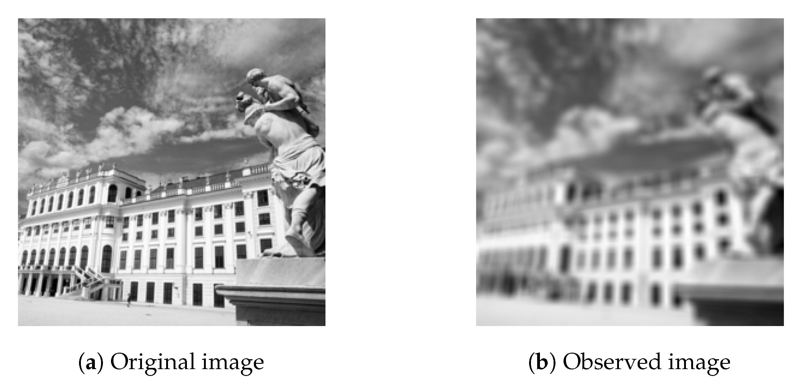
where $x\in {\mathbb{R}}^n$ is the original image, b is the observed image and A represents the blurring operator. In this situation, we choose the regularization parameter $\lambda =5e^{-5}$. For this example, we look at the 256 × 256 Schonbrunn palace (original image). We use a Gausssian blur of size 9 × 9 and standard deviation $\sigma =4$ to create the blurred and noisy image (observed image). These two images are given as in Figure 1.

In 2009, Thung and Raveendran [27] introduced Peak Signal-to-Noise Ratio (PSNR) to measure a quality of restored images for each $x_n$ as the following:

$$PSNR\left(x_n\right)=10log\left(\frac{{255}^2}{MSE}\right),$$

where $MSE=\frac{1}{{256}^2}{\parallel x_n-x\parallel }^2,$ the Mean Square Error for the original image x. We note that a higher PSNR shows a higher quality for deblurring image.

In Theorem 2, we set $h\left(x\right)={\parallel Ax-b\parallel }_2^2$ and $g\left(x\right)={\lambda \parallel x\parallel }_1$ and choose the Lipschitz constant L of the gradient $\nabla h$ which is the maximum value of eigenvalues of the matrix $A^{T}A$.

Let us begin with the first experiment. We study convergence behavior of our method by considering the following six different cases:

Parameters	Case (a)	Case (b)	Case (c)	Case (d)	Case (e)	Case (f)
${\alpha }_n$	$\frac{1}{33n}$	$\frac{1}{33n}$	$\frac{1}{33n}$	$\frac{1}{33n}$	$\frac{1}{33n}$	$\frac{1}{33n}$
${\beta }_n$	$\frac{n}{n+1}$	$\frac{n}{300n+1}$	$\frac{n}{300n+1}$	$\frac{n}{300n+1}$	$\frac{n}{300n+1}$	$\frac{n}{300n+1}$
${\gamma }_n$	$1-{\alpha }_n-{\beta }_n$	$1-{\alpha }_n-{\beta }_n$	$1-{\alpha }_n-{\beta }_n$	$1-{\alpha }_n-{\beta }_n$	$1-{\alpha }_n-{\beta }_n$	$1-{\alpha }_n-{\beta }_n$
${\sigma }_n$	$\frac{n}{10(n+1)}$	$\frac{n}{10(n+1)}$	$\frac{99n}{100(n+1)}$	$\frac{99n}{100(n+1)}$	$\frac{99n}{100(n+1)}$	$\frac{99n}{100(n+1)}$
${\eta }_n$	$\frac{33·{10}^{20}}{n}$	$\frac{33·{10}^{20}}{n}$	$\frac{33·{10}^{20}}{n}$	$\frac{33·{10}^{20}}{n}$	$\frac{33·{10}^{20}}{n}$	$\frac{33·{10}^{20}}{n}$
${\lambda }_n$	$\frac{n}{L(n+1)}$	$\frac{n}{L(n+1)}$	$\frac{n}{L(n+1)}$	$\frac{31n}{20L(n+1)}$	$\frac{31n}{20L(n+1)}$	$\frac{31n}{20L(n+1)}$
$\theta$	0.5	0.5	0.5	0.5	0.09	0.99

It is clear that these control parameters satisfy all conditions of Theorem 2. In this experiment, we take $f\left(x\right)=0.25·x$. By Theorem 2, the sequence $\left\{x_n\right\}$ converges to the original image and its convergence behavior for each case is shown by the values of PSNR as seen in

Table 1. The values of PSNR of six cases in Theorem 2 at $x_1$, $x_5$, $x_{10}$, $x_{25}$, $x_{50}$, $x_{100}$, $x_{250}$, $x_{500}$.

No. Iterations	Case (a)	Case (b)	Case (c)	Case (d)	Case (e)	Case (f)
1	19.435266	19.440476	19.528889	19.686937	19.686937	19.686937
5	20.539773	20.568442	20.849492	21.151064	20.888207	21.598216
10	21.126851	21.174059	21.606305	22.068696	21.554700	23.435160
25	22.136789	22.228847	22.949968	23.587612	22.788089	25.383824
50	23.125241	23.246531	24.087158	24.748261	23.893124	27.283463
100	24.198479	24.331965	25.199378	25.852069	25.000206	29.440357
250	25.605450	25.741976	26.608033	27.265159	26.408127	31.342524
500	26.645135	26.784026	27.674898	28.365891	27.466181	32.443743

.

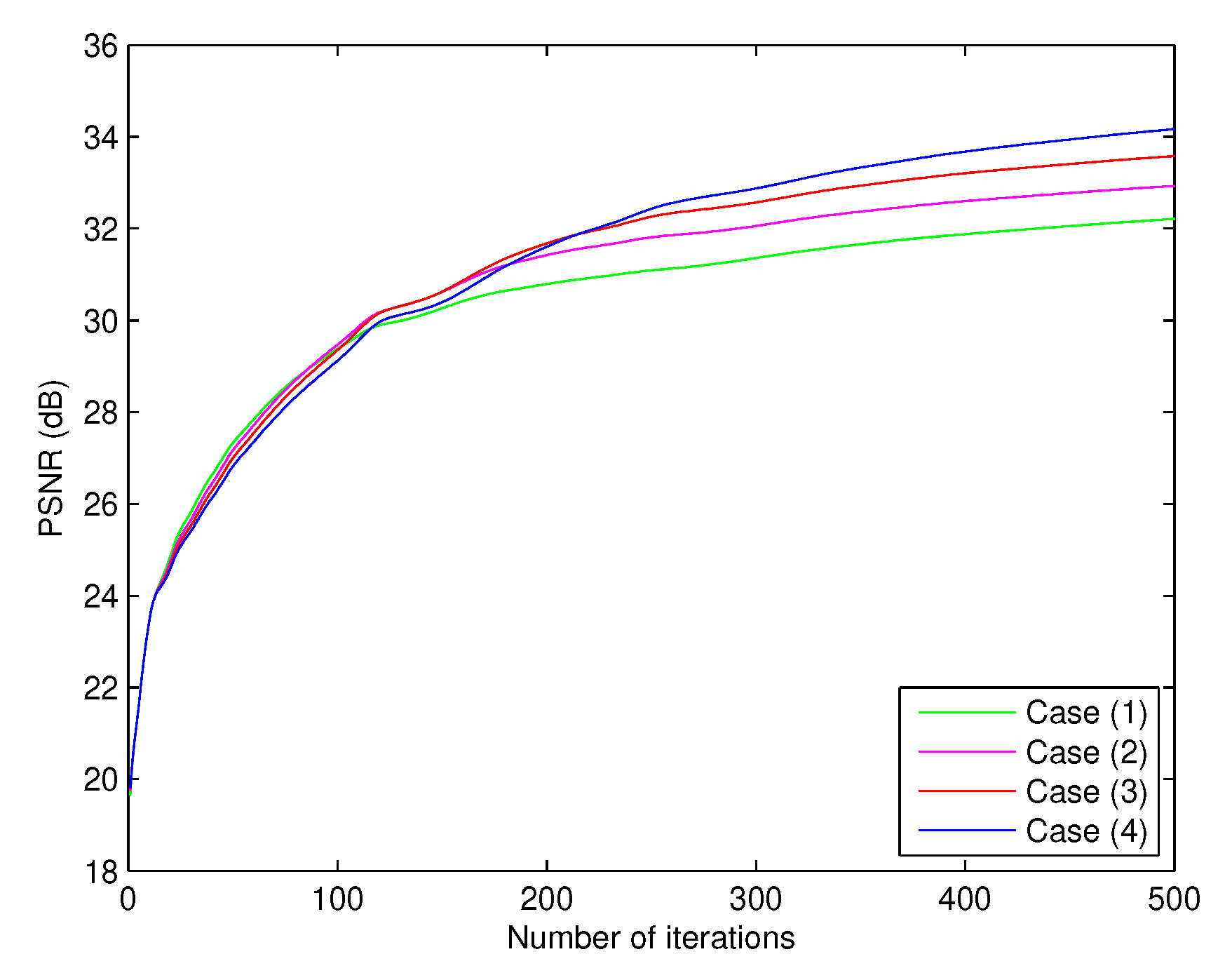
The second experiment is to consider the behavior of the sequence $\left\{x_n\right\}$ for each case of contraction mappings $f\left(x\right)=k·x$. We consider the following four different cases as follows:

Case (1)	$f\left(x\right)=0.1·x$
Case (2)	$f\left(x\right)=0.5·x$
Case (3)	$f\left(x\right)=0.75·x$
Case (4)	$f\left(x\right)=0.95·x$

We choose the parameters as follows:

$${\alpha }_n=\frac{1}{33n},{\beta }_n=\frac{n}{300n+1},{\gamma }_n=1-{\alpha }_n-{\beta }_n,{\sigma }_n=\frac{99n}{100(n+1)},{\eta }_n=\frac{33·{10}^{20}}{n},{\lambda }_n=\frac{31n}{20L(n+1)}.$$

Here $\theta =0.99$ then ${\theta }_n=\left\{\begin{array}{cc}{\displaystyle min\left\{0.99,\frac{{10}^{20}}{n^2\parallel x_n-x_{n-1}\parallel }\right\}}\hfill & \mathrm{if}{x}_n\ne x_{n-1};\hfill \\ 0.99\hfill & \mathrm{otherwise}.\hfill \end{array}\right.$

From

Table 2. The values of PSNR of four cases in Theorem 2 at $x_1$, $x_5$, $x_{10}$, $x_{25}$, $x_{50}$, $x_{100}$, $x_{250}$, $x_{500}$.

No. Iterations	Case (1)	Case (2)	Case (3)	Case (4)
1	19.645629	19.742816	19.781947	19.800875
5	21.595741	21.600924	21.601822	21.601207
10	23.430366	23.441553	23.445829	23.447628
25	25.433348	25.289174	25.178923	25.079196
50	27.329109	27.167872	26.997762	26.819210
100	29.375156	29.468395	29.352150	29.121785
250	31.091760	31.811123	32.260577	32.431003
500	32.212326	32.929758	33.580650	34.170032

, we get the values of PSNR at $x_{500}$ of each case which equal to 32.212326, 32.929758, 33.580650 and 34.170032, respectively. We also observe from Table 2 and Figure 2 that when k is close to 1, the value of PSNR is higher than those of smaller k.

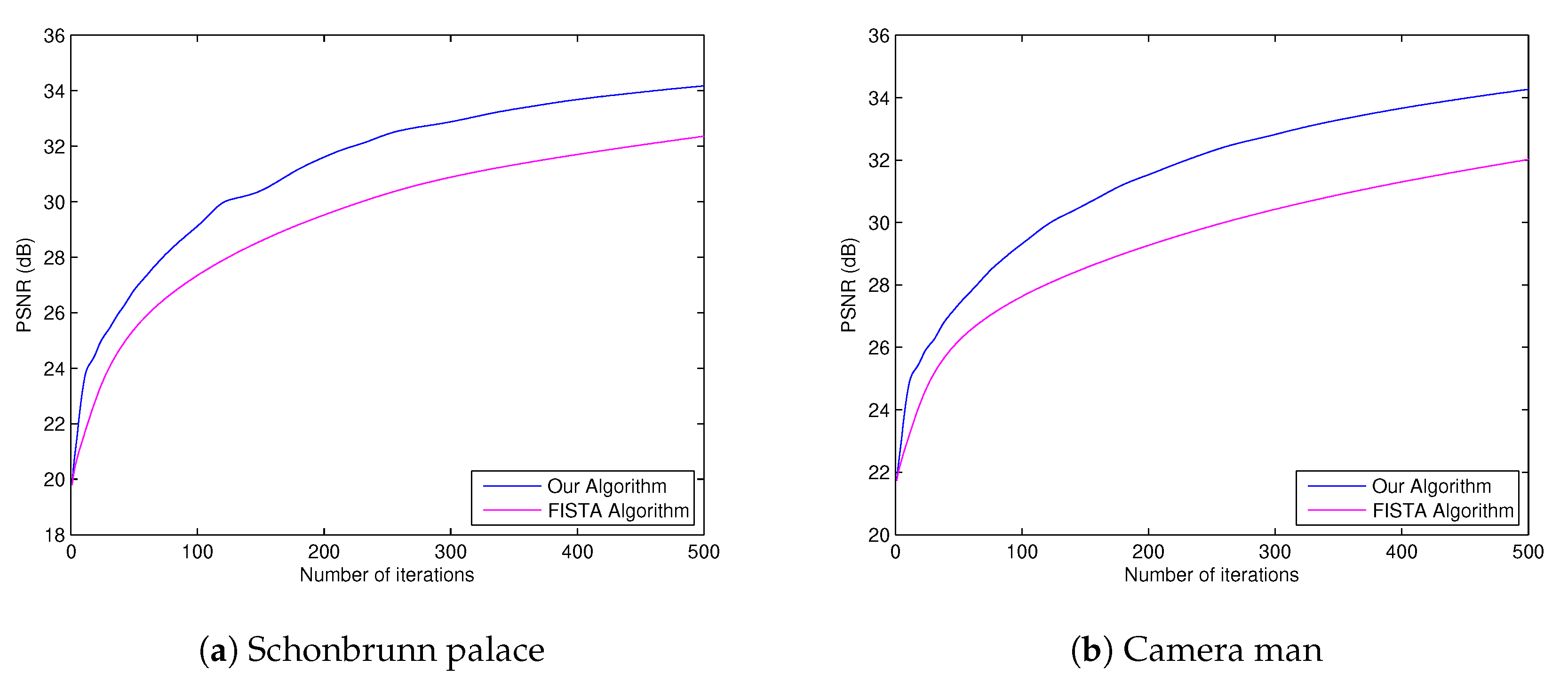
On the other hand, the other experiment is to compare the quality of image restored by our algorithm and the quality of image restored by FISTA method [3]. Here, all parameters in Theorem 2 were the same as the previous experiment and we used $f\left(x\right)=0.95·x$.

For FISTA method [3], we set

$$h\left(x\right)={\parallel Ax-b\parallel }_2^2,g\left(x\right)=\lambda {\parallel x\parallel }_1\mathrm{and}T={\mathrm{prox}}_{\lambda g}(I-\lambda \nabla h),$$

where the parameter $\lambda =\frac{1}{L}.$

Then we obtain the PSNR values of our algorithm and of FISTA as seen in

Table 3. The values of PSNR at $x_1$, $x_5$, $x_{10}$, $x_{25}$, $x_{50}$, $x_{100}$, $x_{250}$, $x_{500}$ (Schonbrunn palace).

No. Iterations	Our Algorithm	FISTA Method
1	19.800875	19.785363
5	21.601207	20.774354
10	23.447628	21.530504
25	25.079196	23.502806
50	26.819210	25.401943
100	29.121785	27.342763
250	32.431003	30.290802
500	34.170032	32.356010

and

Table 4. The values of PSNR at $x_1$, $x_5$, $x_{10}$, $x_{25}$, $x_{50}$, $x_{100}$, $x_{250}$, $x_{500}$ (Camera man).

No. Iterations	Our Algorithm	FISTA Method
1	21.738865	21.730405
5	23.165748	22.429808
10	24.702169	23.081284
25	25.986847	24.741192
50	27.383389	26.213578
100	29.320097	27.633632
250	32.287817	29.889833
500	34.262873	32.016958

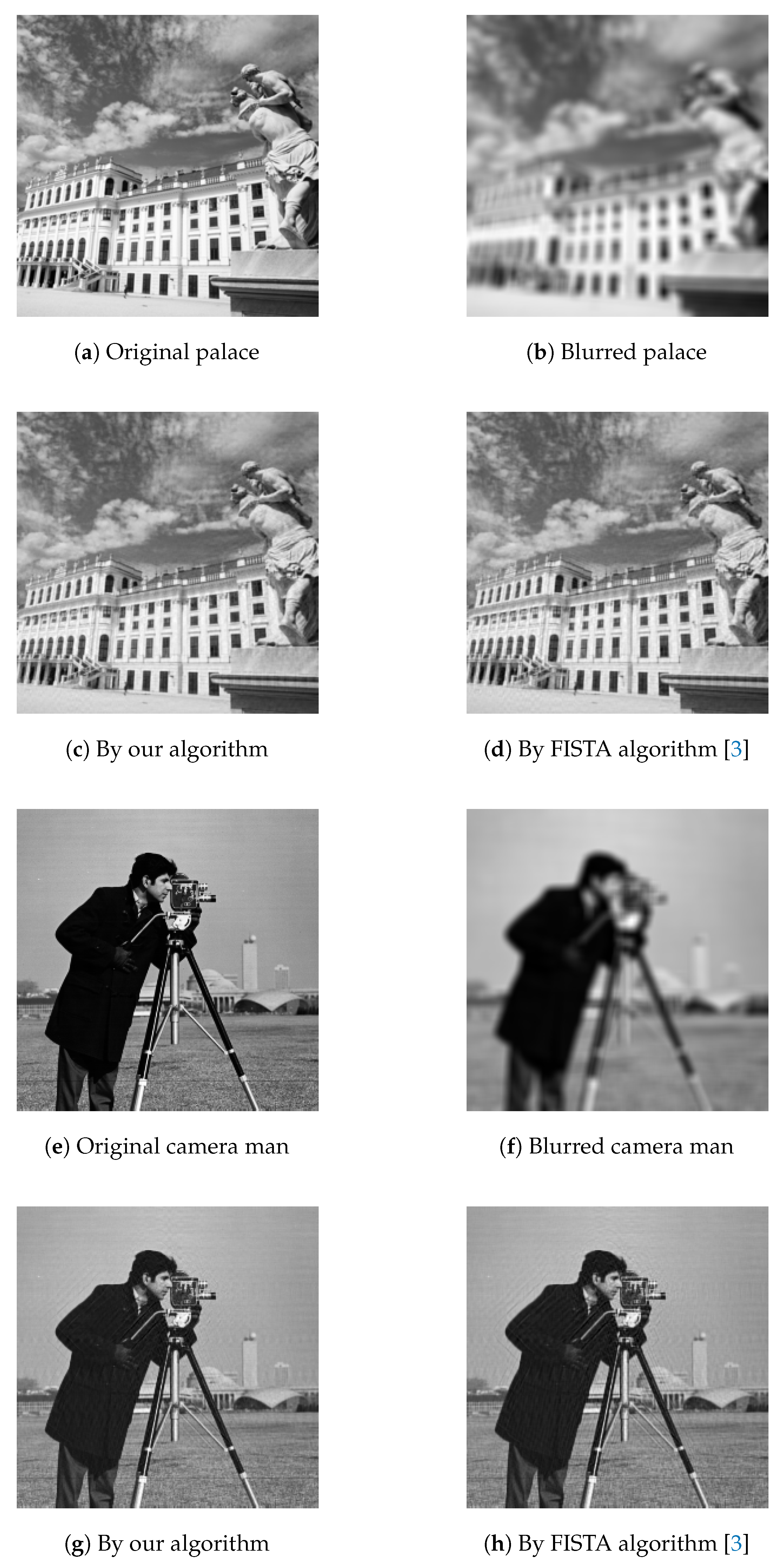
, and Figure 3. The restoration images at 500th iteration of both algorithms are also presented in Figure 4.

Our experiments show that our algorithm gives a better performance in restoring the blurred image than that of FISTA [3].

5. Conclusions

In this paper, we present a new accelerated fixed point algorithm using the ideas of the viscosity and inertial technique to solving image restoration problems. A strong convergence theorem of our proposed method, Theorem 1, is established and proved under some suitable conditions. We then compare its convergence behavior with the others by considering its application to an image restoration problem. We find that our algorithm has convergence behavior better than FISTA which is a well-known and popular method using in image restoration problem.

References

1. Tikhonov, A.N.; Arsenin, V.Y. Solution of Ill-Posed Problems; V.H. Winston: Washington, DC, USA, 1977. [Google Scholar]
2. Tibshirani, R. Regression shrinkage and selection via the lasso. J. R. Stat. Soc. Ser. B (Methodol.) 1996, 58, 267–288. [Google Scholar] [CrossRef]
3. Beck, A.; Teboulle, M. A Fast Iterative Shrinkage-Thresholding Algorithm for Linear Inverse Problems. SIAM J. Imaging Sci. 2009, 2, 183–202. [Google Scholar] [CrossRef] [Green Version]
4. Bauschke, H.H.; Combettes, P.L. Convex Analysis and Monotone Operator Theory in Hilbert Spaces, 2nd ed.; Incorporated; Springer: New York, NY, USA, 2017. [Google Scholar]
5. Parikh, N.; Boyd, S. Proximal Algorithms. Found. Trends® Optim. 2014, 1, 127–239. [Google Scholar] [CrossRef]
6. Mann, W.R. Mean value methods in iteration. Proc. Am. Math. Soc. 1953, 4, 506–510. [Google Scholar] [CrossRef]
7. Reich, S. Weak convergence theorems for nonexpansive mappings in Banach spaces. J. Math. Anal. Appl. 1979, 67, 274–276. [Google Scholar] [CrossRef] [Green Version]
8. Moudafi, A. Viscosity approximation method for fixed-points problems. J. Math. Anal. Appl. 2000, 241, 46–55. [Google Scholar] [CrossRef] [Green Version]
9. Verma, M.; Sahu, D.R.; Shukla, K.K. VAGA: A novel viscosity-based accelerated gradient algorithm- Convergence analysis and applications. Appl. Intell. 2018, 48, 2613–2627. [Google Scholar] [CrossRef]
10. Nesterov, Y. A method for solving the convex programming problem with convergence rate (1/k2). Dokl. Akad. Nauk SSSR 1983, 269, 543–547. [Google Scholar]
11. Rockafellar, R.T. On the maximal monotonicity of subdifferential mappings. Pac. J. Math. 1970, 33, 209–216. [Google Scholar] [CrossRef] [Green Version]
12. Lions, P.L.; Mercier, B. Splitting algorithms for the sum of two nonlinear operators. SIAM J. Numer. Anal. 1979, 16, 964–979. [Google Scholar] [CrossRef]
13. Passty, G.B. Ergodic convergence to a zero of the sum of monotone operators in Hilbert space. J. Math. Anal. Appl. 1979, 72, 383–390. [Google Scholar] [CrossRef] [Green Version]
14. Tseng, P. A modified forward-backward splitting method for maximal monotone mappings. SIAM J. Control Optim. 2000, 38, 431–446. [Google Scholar] [CrossRef]
15. Combettes, P.L.; Hirstoaga, S.A. Equilibrium programming in Hilbert spaces. J. Nonlinear Convex Anal. 2005, 6, 117–136. [Google Scholar]
16. Lopez, G.; Martin-Marquez, V.; Wang, F.; Xu, H.K. Forward-backward splitting methods for accretive operators in Banach spaces. Abstr. Appl. Anal. 2012. [Google Scholar] [CrossRef] [Green Version]
17. Takahashi, W. Introduction to Nonlinear and Convex Analysis; Yokohama Publishers: Yokohama, Japan, 2009. [Google Scholar]
18. Takahashi, W. Nonlinear Functional Analysis; Yokohama Publishers: Yokohama, Japan, 2000. [Google Scholar]
19. Goebel, K.; Reich, S. Uniform Convexity, Hyperbolic Geometry, and Nonexpansive Mappings; Marcel Dekker: New York, NY, USA, 1984. [Google Scholar]
20. Nakajo, K.; Shimoji, K.; Takahashi, W. Strong convergence to a common fixed point of families of nonexpansive mappings in banach spaces. J. Math. Anal. Appl. 2007, 8, 11–34. [Google Scholar]
21. Takahashi, W. Viscosity approximation methods for countable families of nonexpansive mappings in banach spaces. Nonlinear Anal. 2009, 70, 719–734. [Google Scholar] [CrossRef]
22. Bussaban, L.; Suantai, S.; Kaewkhao, A. A parallel inertial S-iteration forward-backward algorithm for regression and classification problems. Carpathian. J. 2020, 36, 35–44. [Google Scholar]
23. Goebel, K.; Kirk, W.A. Topics in Metric Fixed Point Theory; Cambridge Studies in Advanced Mathematics; Cambridge University Press: Cambridge, UK, 1990; Volume 28. [Google Scholar]
24. Aoyama, K.; Yasunori, Y.; Takahashi, W.; Toyoda, M. On a strongly nonexpansive sequence in a Hilbert space. J. Nonlinear Convex Anal. 2007, 8, 471–489. [Google Scholar]
25. Xu, H.K. Another control condition in an iterative method for nonexpansive mappings. Bull. Aust. Math. Soc. 2002, 65, 109–113. [Google Scholar] [CrossRef] [Green Version]
26. Mainge, P.E. Strong convergence of projected subgradient methods for nonsmooth and nonstrictly convex minimization. Set-Valued Anal. 2008, 16, 899–912. [Google Scholar] [CrossRef]
27. Thung, K.-H.; Raveendran, P. A Survey of Image Quality Measures. In Proceedings of the IEEE Technical Postgraduates (TECHPOS) International Conference, Kuala Lumpur, Malaysia, 14–15 December 2009; pp. 1–4. [Google Scholar]
Figure 1. Original image
Mathematics 08 00615 g001
Figure 2. Comparison of four cases in Theorem 2.
Mathematics 08 00615 g002
Figure 3. Schonbrunn palace
Mathematics 08 00615 g003
Figure 4. Original palace
Mathematics 08 00615 g004