Abstract
In this paper, we derive and propose basic differential operations and generalized Green’s integral theorems applicable to multidimensional spaces based on Cartesian tensor analysis to solve some nonlinear problems in smooth spaces in the necessary dimensions. In practical applications, the theorem can be applied to numerical analysis in the conservation law, effectively reducing the dimensions of high-dimensional problems and reducing the computational difficulty, which can be effectively used in the solution of complex dimensional mechanical problems.
1. Introduction
In modern mathematical systems, the research on vectors and tensors is a hot topic. The analysis of both has been applied in many new subject areas, not only in the field of pure mathematics [1,2], but in the mechanics field [3,4] and engineering extending from these areas [5]. Vector analysis is a branch of mathematics that extends the method of mathematical analysis to two-dimensional or three-dimensional vectors [6,7,8,9]. Tensor analysis is a combination of generalization and tensor of vector analysis. It studies the differential operators in the differential domain D (M). Therefore, trying to combine the usual differential integration operations and some differential operators with vector tensor analysis can improve the efficiency of the calculation or reduce the difficulty of the calculation. For example, in continuum mechanics, some physical quantities are vectors and tensors or their functions. If we want to study mathematical models related to continuum mechanics, the research on the related vector tensor inside the model will allow us to better understand the laws of the model and even reveal the motion of certain non-linear physical quantities; because there are many non-linear systems in engineering problems, the study of vector tensor analysis has important engineering significance [10].
Specifically, this research can also solve some scientific problems. For example, engineering problems always involve issues such as elastic mechanics [11], electrodynamics [12], fluid mechanics [13], and other fields of mechanics. These fields are built around characteristic equations, such as the Navier–Stokes equation for fluid mechanics, the Maxwell equation for electrodynamics, and the Hamilton equation for analytical mechanics. From the perspective of algebra, these characteristic equations can be regarded as scalars, vectors, and tensors in the Cartesian coordinate system. Therefore, the research of vector tensor analysis is helpful for studying the fundamental meaning of vector tensor operations, and it can promote the development of applied mathematics and related mechanics fields, thereby solving scientific problems in engineering. However, the vector tensor operations in the Cartesian coordinate system still have certain limitations. For example, for the research of second-order operators, only the properties of basic operators such as the Laplace operator are obtained, which hinders our study. Therefore, in this paper, we hope to study the properties of common operators in continuum mechanics and solve some engineering problems.
In the current research on continuum mechanics, according to the continuity assumption, in mathematics, continuum mechanics is an expression consisting of vector, tensor, and scalar systems. Therefore, developing tensor analysis in Cartesian coordinates can help to promote the development of continuum mechanics. As we all know, the boundary element method (BEM) is an effective numerical method. This method is based on the boundary integral equation, which can simplify the calculation of the solution domain to the boundary calculation. Therefore, this method is successfully used to solve the cases of the complex plane, space, and fixed and non-stationary engineering problems. Many studies based on BEM have proven that the boundary element method plays a significant role in the solution of viscous fluid linear and nonlinear problems, as well as convergence and error analysis. However, during the research, we found that the boundary element method has certain limitations in high Reynolds number fluids, such as turbulence, which is specifically reflected in the inaccurate calculation results. We believe that the problem lies in the calculation of points. Therefore, we considered the characteristics of the integral calculation by the boundary element method, studied the integral operator based on the Green’s formula, generalized the integral calculation, and derived the generalized Green’s formula to solve the related problems.
2. Definition and Base Vector for the Auxiliary Space
There will be some operators defined in this paper. The meaning and calculation rules of these operators will be introduced here.
Definition 1.
Let the existence normed vector space , ,
- (a)
- if mappings f and g are satisfied:
- (1)
- =
- (2)
- =
- (3)
- = =then mapping is defined as .
- (b)
- if mappings f and g are satisfied:
- (1)
- = 0
- (2)
- =
- (3)
- = =then mapping is defined as .
The curly braces do not represent any operators; they just separate the vectors in the equation. Currently, there are many feature geometries that we cannot describe with two-dimensional geometry, that is vectors , such as vorticity. Therefore, we need to define auxiliary space to represent it to introduce curl in two dimensions. In Cartesian coordinates, operations (,) and [,] can be seen as dot multiplication and cross-multiplication, satisfying all algorithms of dot multiplication and cross-multiplication for modern vectors and tensors analysis.
Definition 2.
Let existence normed vector space and ,
then normed vector space K is the auxiliary space of Ω. When , then is defined by the base vector in K. The space consisting of Ω and K is defined as .
The base vector can be analogized to the normal vector of a two-dimensional plane, that is on a straight line perpendicular to the plane. The purpose of introducing is to locate two-dimensional space in three-dimensional space. is the dyad of .
The unit vectors are , and , where is the normal vector of the plane where the vectors and lie (Figure 1) [6], and corresponds to one-to-one.
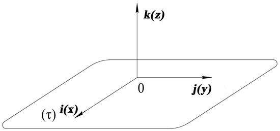
Figure 1.
Positional relationship of vectors and .
In summary, referring to the the research of Krashanitsa [9] and Kochin [14], this paper proposes a generalized Green’s formula, which can be used to solve complex problems related to continuous mechanics further, to solve nonlinear problems, and can be used to promote the development of applied mathematics related content, which has great theoretical and engineering significance.
3. Generalization of the Tensor Analysis Differential Calculation Form
In classical field theory, we can use vector and field theory analysis in Cartesian coordinates for the description of continuum mechanics. Therefore, we can write down the following generalized differential operation of vector tensor analysis performed using operator ∇.
Lemma 1.
Let , K be the auxiliary space of Ω, manifold , and , and be the basic vector of auxiliary space K, then the following identity relationship can be proven.
where and are conjugate tensors, which with the help of the basic vectors and of the two-dimensional system can be expressed as:
As a famous vector analysis theorem [6,7,8], we can write out the second lemma.
Lemma 2.
Let , manifold , , and ; the following relationships can be proven:
Theorem 1.
Let , K be the auxiliary space of Ω, manifold , , and , and be the basic vector of auxiliary space K. If can be expressed as:
then the following equation exists:
Proof.
By virtue of , the second partial derivatives of and are continuous. For a more intuitive understanding, in two dimensions, we can prove it with the help of the basic vectors and in two-dimensional space. At this time, vectors and can be expressed as:
Theorem 2.
Let , K be the auxiliary space of Ω, manifold , , and be the basic vector of auxiliary space K:
Proof.
and the poof is completed. □
We substitute tensor and scalar into Equation (3), and for , K is the auxiliary space of , manifold , is the basic vector of auxiliary space K. We can get:
Multiplying both sides of the equal sign by the normal unit vector for an arbitrary curve in gives:
The second expression to the right of the equal sign can be simplified by (4):
Therefore, Equation (7) can be transformed into:
Theorem 3.
Let , K be the auxiliary space of Ω, manifold , and , be the basic vector of auxiliary space K, and be the normal unit vector for arbitrary curve in Ω.
4. Generalized Integral Theorem for Tensor Analysis
In continuum mechanics or classical physics, many famous partial differential equations can be formulated as the operator form , for example the Navier–Stokes equation in fluid mechanics and Maxwell’s equations in electrodynamics. Therefore, it is necessary to study the properties of the operator mathematically.
Definition 3.
Let , manifold , , , and . Then, the fundamental equation in mechanics can be expressed as:
where and are vectors and tensors related to the solution of specific problems in mechanics.
Theorem 4.
Let , manifold , , and .
Proof.
The left side of the equation can be written as:
expanded in Cartesian coordinates, where the first item can be expressed as:
the second item can be expressed as:
then from the first item minus the second item, we can obtain:
and the poof is completed. □
Therefore, these operators operating on the domain () can be obtained as:
According to the generalized Stokes theorem [15], for , we can write the following transformations:
After a simple vector operation, we obtain:
where = in Figure 2. In order to get a more widely useful theorem, we give a common lemma.
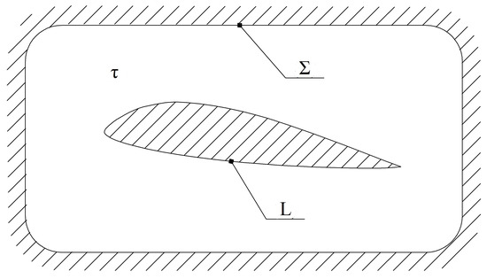
Figure 2.
The position of the region with the boundaries and L.
Lemma 3.
Let , manifold , , , and be the normal vector of the boundary , so:
Proof.
Utilizing the basic vectors in two-dimensional Cartesian space, the left side of the equation can be expressed as:
and the poof is completed. □
Combined with the above derivations, the generalized Green integral theorem has the following form:
Theorem 5.
Let , manifold , , and , and be the normal vector of the boundary , so:
According to the generalized Stokes theorem [6,8], we can write the following form:
5. Properties of the Conjugate Normal Derivative
However, in the actual application process, we hope to get its own operation. Therefore, we need to study the basic properties of “*”.
Lemma 4.
Let , manifold , , and be the normal vector of the boundary , so:
or it can be written as:
Proof.
In the Cartesian coordinate system, we use the basic vectors to represent:
or we can express it in another way:
and the poof is completed. □
Lemma 5.
Let , manifold , , and be the normal vector of the boundary .
Simultaneously, Theorem (13), (14), and (15) can be obtained:
Theorem 6.
Let , manifold , , , and be the normal vector of the boundary .
Multiplying the theorem (17) on the left and right by the scalar , we have:
Theorem 7.
Let , K be the auxiliary space of Ω, manifold , and , be the basic vector of auxiliary space K, and be the normal vector of the boundary .
Proof.
Consistent with the above, we still choose to represent the left of (18) in Cartesian coordinates.
and the poof is completed. □
For any vector a, b, and c, the following theorem holds:
Therefore, let , manifold , and , and be the normal vector of the boundary .
Theorem 8.
Let , K be the auxiliary space of Ω, manifold , and , be the basic vector of auxiliary space K, and be the normal vector of the boundary .
Simultaneously, Theorem (12) can be obtained:
Theorem 9.
Let , K be the auxiliary space of Ω, manifold , and , be the basic vector of auxiliary space K, and be the normal vector of the boundary .
and decomposition property of the integral:
6. Paper Summary and Prospects for the Future
Based on some existing tensor theorems, this paper proved and derived the relationship between some vector and tensor theorems, obtained the conjugate derivative with respect to the normal vector, and finally proposed the generalized Green’s theorem. This theorem has great theoretical and practical significance in solving continuum mechanics problems and can promote the solution of initial boundary value problems in fluid dynamics, elasticity, and plasticity. Furthermore, the aerodynamic characteristics of an aircraft in different environmental flowing media can be solved, and combined with the relevant research content of the aerodynamic characteristics of the wing, it can help solve the problem of instability that may occur when the aircraft takes off and lands. With the help of the generalized Green’s theorem proposed in this paper, the dimensionality reduction of complex dimensional problems can be solved, which further eliminates the complex calculation problems that may arise during the calculation process and makes it easier to solve complex dimensional engineering problems.
Author Contributions
Conceptualization, P.Y.; methodology, P.Y., Y.L. and S.W.; validation, Y.L. and S.W.; formal analysis, S.W.; investigation, Y.L.; resources, P.Y.; writing–original draft preparation, Y.L., P.Y. and S.W.; writing–review and editing, Y.L., P.Y. and S.W.; visualization, Y.L.; supervision, P.Y. and S.W.; project administration, P.Y.; funding acquisition, P.Y. All authors have read and agreed to the published version of the manuscript.
Funding
Sichuan Expert Service Center: M162019LXHGKJHD18; University of Electronic Science and Technology of China: A03019023801181, Y030202059018010. APC is funded by “ New Engineering ” undergraduate scientific research education project of the School of Aeronautics and Astronautics, University of Electronic Science and Technology of China: Y03019023701002377.
Acknowledgments
This research was supported by SiChuan Provincial Expert Service Center, Excellent researchers upon the key projects, M162019LXHGKJHD18; University of Electronic Science and Technology of China (Central Financial Project in China), Research Startup Fund, Y030202059018010, Basic service fond of central university, A03019023801181, “New Engineering” research and education project for undergraduate, Y03019023701002377. Thanks to these organizations for supporting the project research. We would like to pay tribute to professor Krashanitsya for selfless help in the project.
Conflicts of Interest
The authors declare no conflicts of interest.
References
- Wrede, R.C. Introduction to Vector and Tensor Analysis; Courier Corporation: Chelmsford, UK, 2013. [Google Scholar]
- Arnoldus, S.J. Ricci-Calculus: An Introduction to Tensor Analysis and Its Geometrical Applications; Springer Science & Business Media: Berlin, Germany, 2013. [Google Scholar]
- Talpaert, Y.R. Tensor Analysis and Continuum Mechanics; Springer Science & Business Media: Berlin, Germany, 2013. [Google Scholar]
- Lebedev, L.P.; Cloud, M.J.; Eremeyev, V.A. Tensor Analysis with Applications in Mechanics; World Scientific: Singapore, 2010. [Google Scholar]
- Abraham, R.; Marsden, J.E.; Ratiu, T. Manifolds, Tensor Analysis, and Applications; Springer Science & Business Media: Berlin, Germany, 2012. [Google Scholar]
- Hackbusch, W. Tensor Spaces and Numerical Tensor Calculus; Springer: Berlin, Germany, 2012. [Google Scholar]
- Eremeyev, V.A.; Cloud, M.J.; Lebedev, L.P. Applications of Tensor Analysis in Continuum Mechanics; World Scientific: Singapore, 2019. [Google Scholar]
- Krashanitsa, Y.A. Development of hydrodynamic potentials theory and the method of boundary-integral equations in hydrodynamics problems. Act. Prob. Aviat. Aerospace Syst. Processes Models Exp. 2013, 18, 37. [Google Scholar]
- Huang, K. Tensor Analysis; Beijing Higher Education Publishing: Beijing, China, 1998. [Google Scholar]
- Vectors, A.R. Tensors and the Basic Equations of Fluid Mechanics; Courier Corporation: Chelmsford, UK, 2012. [Google Scholar]
- Ogden, R.; Steigmann, D. Mechanics and Electrodynamics of Magneto- and Electro-Elastic Materials; Springer Science & Business Media: Berlin, Germany, 2011. [Google Scholar]
- Turowski, J.; Turowski, M. Engineering Electrodynamics: Electric Machine, Transformer, and Power Equipment Design; CRC Press: New York, NY, USA, 2017. [Google Scholar]
- Yamaguchi, H. Engineering Fluid Mechanics; Springer Science & Business Media: Berlin, Germany, 2008. [Google Scholar]
- Kochin, N.E. Vector Calculus and the Beginnings of Tensor Calculus; USSR Academy of Sciences: Moscow, Russia, 1961; p. 427. [Google Scholar]
- Ladopoulos, E.G. Non-linear multidimensional singular integral equations in two-dimensional fluid mechanics. Int. J. Non-Linear Mech. 2000, 35, 701–708. [Google Scholar] [CrossRef]
© 2020 by the authors. Licensee MDPI, Basel, Switzerland. This article is an open access article distributed under the terms and conditions of the Creative Commons Attribution (CC BY) license (http://creativecommons.org/licenses/by/4.0/).