A Density-Dependent Host-Parasitoid Model with Stability, Bifurcation and Chaos Control

Abstract

The aim of this article is to study the qualitative behavior of a host-parasitoid system with a Beverton-Holt growth function for a host population and Hassell-Varley framework. Furthermore, the existence and uniqueness of a positive fixed point, permanence of solutions, local asymptotic stability of a positive fixed point and its global stability are investigated. On the other hand, it is demonstrated that the model endures Hopf bifurcation about its positive steady-state when the growth rate of the consumer is selected as a bifurcation parameter. Bifurcating and chaotic behaviors are controlled through the implementation of chaos control strategies. In the end, all mathematical discussion, especially Hopf bifurcation, methods related to the control of chaos and global asymptotic stability for a positive steady-state, is supported with suitable numerical simulations.

1. Introduction

The host-parasitoid interaction is the most underlying and substantial procedure in population dynamics. Many species, such as semelparous animals and monocarpic plants, have discrete seasonal (non-overlapping) generations and their births take place in customary reproduction seasons. Their interactions are described by difference equations or formulated as discrete-time mappings.

Discrete-time models are widely used to explore the dynamics of host-parasitoid interactions in an ecosystem. In nature, most of host-parasitoid systems have complexity due to the interaction of species. On the other hand, in most of such cases, the coexistence of both species is mostly stable. We propose a host-parasitoid model with the implementation of a Beverton-Holt growth function for the host population and Hassell-Varley framework to make the coexistence stable. On the other hand, chaotic behavior is also observed for the proposed model. In the case of ecological models related to the breeding of biological species, chaos is considered as irregular and unpredictable behavior; therefore, the presence of chaos is an unfavorable situation for the survival of a species [1]. Thus, chaos control methods can be used by the species to avoid risks of irregular behavior. Qualitative analysis for various classes of host-parasitoid interaction is a topic of great interest. Recently, many researchers have focused their studies on the dynamics of host-parasitoid models. Some of these investigations, which are very close to the present study, are summarized as follows. Taylor [2] investigated the dynamics of some host-parasitoid systems under competition. Kaitala et al. [3] discussed a comprehensive study of the complex dynamics occurring in a basic discrete-time model of host-parasitoid interaction. Tang and Chen [4] applied Holling type II and III functional response functions to a host-parasitoid model. Xu and Boyce [5] reported that mutual interference in host-parasitoid interaction not only can stabilize the dynamics but may strongly destabilize as well. Lv and Zhao [6] studied the complex dynamics in a discrete-time model of host-parasitoid interaction based on a lower bound for the host. Din [7] investigated global dynamics for a class of host-parasitoid systems related to plant-herbivore interaction with strong predator functional response. Din [8] modified the host-parasitoid interaction with implementation of constant refuge effects and reported global dynamics for the proposed model. In [9], the authors modified the host-parasitoid interaction with a Pennycuick growth function for the host population and studied Neimark-Sacker bifurcation and chaos control. In [10], global stability and Hopf bifurcation were carried out for a class of host-parasitoid interaction. Din [11] reported Neimark-Sacker bifurcation and chaos control in a Hassell-Varley model. Global dynamics and Neimark-Sacker bifurcation were investigated for Beddington and generalized Beddington models in [12] and [13], respectively. Global stability, bifurcation analysis and control for host-parasitoid interactions were reported in [14] and [15]. Wu and Zhao [16] studied the qualitative behavior of a discrete host-parasitoid model with the host subjected to refuge and strong Allee effects. Jamieson [17] discussed global dynamics of the May host-parasitoid interaction. Liu et al. [18] explored a complex behavior and bifurcation analysis for a class of host-parasitoid interaction with an application of the Allee effect and Holling type III functional response. Moreover, in [19], chaos control and bifurcation analysis were studied for a host-parasitoid model with a lower bound for the host. In [20] and [21], the influence of a refuge effect was explored for certain classes of host-parasitoid models. In [22], the authors numerically investigated a system of partial differential equations that describe the interactions between populations of predators and prey. Suryanto et al. [23] considered a model of predator-prey interaction at fractional-order with a ratio-dependent functional response. Zhang et al. [24] reported dynamics of a predator-prey system with the weak Allee effect.

Generally, the host-parasitoid interaction is considered as non-overlapping generations. Therefore, difference equations can be used to describe their mathematical framework. One of the pioneer works for mathematical modeling of host-parasitoid interaction was presented by Nicholson and Bailey [25]. The general framework for mathematical modeling of a host-parasitoid system is presented as follows:

$$\begin{array}{ccc}\hfill H_{n+1}& =& r{H}_{n}f(H_n,P_n),\hfill \\ \hfill P_{n+1}& =& c{H}_n\left(1-f(H_n,P_n)\right),\hfill \end{array}$$

where $H_n$ and $P_n$ denote population densities for host and parasitoid, respectively, at the n-th generation; $f(H_n,P_n)$ represents the fraction of host population that does not parasitize; r represents the number of eggs that are laid by a host; and c is used for the intrinsic growth rate of a parasitoid population.

Nicholson and Bailey assume that $f(H_n,P_n)=exp(-a{P}_n)$, which is derived from the zero-th term of the Poisson distribution, where a represents per capita searching efficiency of the parasitoid population. With this particular implementation of $f(H_n,P_n)=exp(-a{P}_n)$, the Nicholson and Bailey model is given as follows:

$$\begin{array}{ccc}\hfill H_{n+1}& =& r{H}_{n}exp(-a{P}_n),\hfill \\ \hfill P_{n+1}& =& c{H}_n\left(1-exp(-a{P}_n)\right).\hfill \end{array}$$

It is worthwhile to note that coexistence is unstable in the case of the Nicholson-Bailey model (NBM). On the other hand, in our universe, most of the host-parasitoid interactions are stable. Therefore, many modifications are suggested to NBM to make its resemblance to natural host-parasitoid systems. For this, it is more appropriate to interchange the constant reproduction rate of hosts to some density-dependent function for the host population. Consequently, the implementation of such density-dependent factors can modify NBM to make its resemblance with the natural host-parasitoid interaction.

Keeping in view the single species density-dependent model for the host population, the Ricker model [26] is a classic discrete population model, which gives the expected number $H_{n+1}$ of individuals in generation $n+1$ as a function of the number of individuals in the previous generation. This model is given as follows:

$$H_{n+1}=H_{n}exp\left(s\left(1-\frac{H_n}{l}\right)\right),$$

where s is interpreted as an intrinsic growth rate and l as the carrying capacity of the environment. The Ricker model was introduced in 1954 by Ricker in the context of stock and recruitment in fisheries. The model can be used to predict the number of fish that will be present in a fishery. Subsequent work has been derived from the model under other assumptions, such as scramble competition, within-year resource-limited competition or even as the outcome of source-sink Malthusian patches linked by density-dependent dispersal. The Ricker model is a limiting case of the Hassell model [27], which takes the form:

$$H_{n+1}=\frac{r{H}_n}{{(1+k{H}_n)}^b},$$

(1)

where $r\ge 1$ denotes the growth rate of the population; $b>0$ is used to represent intra-specific competition; and $k>0$ is a scaling parameter for describing the steady population size. If we take $b=1$ in Equation (1), then the Hassell model is simply the Beverton-Holt model [28] given as follows:

$$H_{n+1}=\frac{r{H}_n}{1+k{H}_n}.$$

(2)

Biological assumptions related to Equation (2) are given as follows [29]:

(i) 

It is assumed that the first encounter between the parasitoid and host is random. Moreover, one viable egg is laid by a parasitoid on a single host, which is killed by the parasitoid’s progeny.

(ii) 

Keeping in view the law of mass action, the number of encounters $H_e$ of resources (hosts) with consumers (parasitoids) in generation n are proportional to the product of hosts and parasitoids present densities, and consequently, one has:

$$H_e:=a{H}_n{P}_n$$

where a is a positive constant representing the searching efficiency of the parasitoid, and $P_n$, $H_n$ denote the population densities of the parasitoid and host, respectively, in generation n.

(iii) 

The next generation of parasitoids is produced due to infection of hosts in the present generation.

(iv) 

The hosts that are not infected produce their own offspring.

Keeping in view the assumptions $\left(i\right)$–$\left(iv\right)$ and the Beverton-Holt model in Equation (2), we have the following system for host-parasitoid interaction:

$$\begin{array}{cc}\hfill H_{n+1}& =\frac{r\left(H_n-H_e\right)}{1+k\left(H_n-H_e\right)},\hfill \\ \hfill P_{n+1}& =c{H}_e,\hfill \end{array}$$

(3)

where c is used for the intrinsic growth rate of the parasitoid population. Due to the randomness of encounters between hosts and parasitoids, it is more appropriate to represent the probability of N encounters by a distribution, which depends on the average number of encounters per unit time. Consequently, this condition leads to implementation of the Poisson distribution, and probability mass function is described as follows:

$$P\left(N\right):=\frac{exp\left(-aP\right){\left(aP\right)}^N}{N!},N=0,1,2,\cdots ,$$

where P represents the number of parasitoids, N denotes the number of encounters per unit time, and $aP$ is used for the mean of the distribution, which represents the average number of encounters per unit time. Therefore, the portion of the hosts without parasitism are given as follows:

$$P\left(0\right):=exp\left(-aP\right).$$

Furthermore, it follows that

$$P_{n+1}=c{H}_e=c{H}_n\left(1-P\left(0\right)\right)=c{H}_n\left(1-exp(-a{P}_n)\right).$$

(4)

Next, from Equation (4), it follows that

$$H_n-H_e:=exp\left(-a{P}_n\right).$$

(5)

Then, from Equations (3)–(5), it follows that:

$$\begin{array}{cc}\hfill H_{n+1}& =\frac{r{H}_{n}exp(-a{P}_n)}{1+k{H}_{n}exp(-a{P}_n)},\hfill \\ \hfill P_{n+1}& =c{H}_n\left(1-exp(-a{P}_n)\right).\hfill \end{array}$$

(6)

Arguing as in [30], one may consider the influence of parasitoid interference on the interaction of the host-parasitoid model. For this, the searching efficiency a of parasitoids can be taken as $a=-q{P}_n^{-m}$, where m is a constant for mutual interference, and q represents the quest constant, which denotes the searching efficiency of the parasitoid as $P_n=1$. Keeping in view the Hassell-Varley modification of the host-parasitoid interaction, System (6) is modified as follows:

$$\begin{array}{cc}\hfill H_{n+1}& =\frac{r{H}_{n}exp\left(-q{P}_n^{1-m}\right)}{1+k{H}_{n}exp\left(-q{P}_n^{1-m}\right)},\hfill \\ \hfill P_{n+1}& =c{H}_n\left(1-exp\left(-q{P}_n^{1-m}\right)\right).\hfill \end{array}$$

(7)

The remaining discussion of this paper is summarized as follows. In Section 2, we discuss the permanence of solutions of System (7). In Section 3, the existence, uniqueness and local stability analysis of the positive fixed point of System (7) are studied. Section 4 is dedicated to examining the parametric conditions for global asymptotic stability of the positive fixed point of System (7). Neimark-Sacker bifurcation about the positive fixed point of System (7) is studied in Section 5 with the implementation of the theory of normal forms. In Section 6, the pole-placement method and hybrid control strategy are implemented for controlling the chaotic and fluctuating behavior of System (7) about its positive fixed point. At the end, numerical simulations are presented to authenticate the mathematical analysis in Section 7. Moreover, theoretical findings are validated through experimental and field data based on statistical analysis of previous literatures.

2. Permanence

In the case of difference equations, the permanence of solutions is an important tool to discuss further dynamical behavior of the equations.

Definition 1.

Suppose $\left\{(H_n,P_n)\right\}$ denotes a positive solution for System (7). Then, we say that System (7) is permanent if the following hold true:

$${\displaystyle m\le \underset{n\to \infty }{lim}inf\left(H_n,P_n\right)\le \underset{n\to \infty }{lim}sup\left(H_n,P_n\right)\le M,}$$

where m and M are some positive constants.

Theorem 1.

Assume that $\left\{(H_n,P_n)\right\}$ is an arbitrary solution of System (7). Moreover, suppose that $exp\left(q{M}_2^{1-m}\right)<r$ and $M_2^m<qc{m}_1$, then the following results hold true:

$${\displaystyle m_1\le \underset{n\to \infty }{lim}inf{H}_n\le \underset{n\to \infty }{lim}sup{H}_n\le M_1,m_2\le \underset{n\to \infty }{lim}inf{P}_n\le \underset{n\to \infty }{lim}sup{P}_n\le M_2,}$$

where

$$M_1:=\frac{r-1}{k},M_2=:c{M}_1,m_1=:\frac{r-exp\left(q{M}_2^{1-m}\right)}{k},m_2=:\frac{qc{m}_1-M_2^m}{qc{m}_1}.$$

(8)

Proof. 

Keeping in view the first equation of Model (7), it follows that $H_{n+1}\le \frac{r{H}_n}{1+k{H}_n}$, then the comparison argument yields that ${\displaystyle \underset{n\to \infty }{lim}sup{H}_n\le \frac{r-1}{k}=M_1}$ for every $n=1,2,\cdots$. Next, the second equation of System (7) gives that $P_{n+1}\le c{H}_n$; therefore, it is easy to see that ${\displaystyle \underset{n\to \infty }{lim}sup{P}_n\le \frac{c(r-1)}{k}=M_2}$ for every $n=1,2,\cdots$. Next, focusing on the first equation of System (7), one has that

$$H_{n+1}\ge \frac{r{H}_n}{e^{q{M}_2^{1-m}}+k{H}_n},n=0,1,2,\cdots .$$

(9)

Next, one can implement the transformation $S_n=1/H_n$ in Inequality (9) to obtain $S_{n+1}\le \alpha +\beta S_n$ for all $n=0,1,2,\cdots$, where $\beta =e^{q{M}_2^{1-m}}/r$ and $\alpha =k/r$. If we suppose that $S_0=1/H_0$ and $\beta <1$, then due to the comparison argument, one has ${\displaystyle m_1:=\frac{1-\beta }{\alpha }\le \underset{n\to \infty }{lim}inf{H}_n}$ for every $n=1,2,\cdots$, and it follows from the fact that ${\displaystyle \underset{n\to \infty }{lim}inf(1/S_n)=\underset{n\to \infty }{lim}sup{S}_n}$. Next, we again focus on the second equation of System (7) and see that $P_{n+1}\ge \frac{qc{m}_1{P}_n}{M_2^m+q{P}_n}$ for every $n=0,1,2,\cdots$. On the other hand, we consider a transformation of the form $P_n=1/Q_n$, then one has $Q_{n+1}\le {\alpha }_1+{\beta }_1{Q}_n$ for every $n=0,1,2,\cdots$, where ${\beta }_1=M_2^m/qc{m}_1$ and ${\alpha }_1=1/c{m}_1$. Furthermore, let $P_0=1/Q_0$ and ${\beta }_1<1$, then it is quite simple to see that ${\displaystyle m_2=(1-{\beta }_1)/{\alpha }_1\le \underset{n\to \infty }{lim}inf{P}_n}$ for all $n=1,2,\cdots$. Consequently, one has the desired results as follows:

$${\displaystyle m_1\le \underset{n\to \infty }{lim}inf{H}_n\le \underset{n\to \infty }{lim}sup{H}_n\le M_1,}$$

and

$${\displaystyle m_2\le \underset{n\to \infty }{lim}inf{P}_n\le \underset{n\to \infty }{lim}sup{P}_n\le M_2.}$$

 □

Next, one can apply Theorem 1 along with mathematical induction to prove the following result:

Lemma 1.

Suppose $r>1$, then the rectangle $\left[0,\frac{r-1}{k}\right]\times \left[0,\frac{c(r-1)}{k}\right]$ is an invariant set for each solution $\left\{\left(H_n,P_n\right)\right\}$ of Model (7).

3. Existence of Positive Fixed Point and Stability Analysis

The equilibria of System (7) satisfy $H=\frac{rHexp\left(-q{P}^{1-m}\right)}{1+kHexp\left(-q{P}^{1-m}\right)}$ and $P=cH\left(1-exp\left(-q{P}^{1-m}\right)\right)$. Obviously, System (7) has a trivial equilibrium $(0,0)$, the second is a boundary equilibrium $\left(\frac{r-1}{k},0\right)$ and a positive equilibrium $(H^{*},P^{*})$, which satisfies $1=\frac{r}{exp\left(q{\left(P^{*}\right)}^{1-m}\right)+k{H}^{*}}$ and $P^{*}=c{H}^{*}\left(1-exp\left(-q{\left(P^{*}\right)}^{1-m}\right)\right)$. The positive equilibrium $(H^{*},P^{*})$ cannot be found in closed form. The following result shows the existence and uniqueness of a positive equilibrium point $(H^{*},P^{*})\in \left[0,\frac{r-1}{k}\right]\times \left[0,\frac{c(r-1)}{k}\right]$ of System (7).

Theorem 2.

Suppose that $0<m<1$ and $r>1$, then there exists an interior fixed point $(H^{*},P^{*})\in \left[0,\frac{r-1}{k}\right]\times \left[0,\frac{c(r-1)}{k}\right]$ for System (7).

Proof. 

In order to show the existence and uniqueness of positive equilibrium, we construct a real-valued function $F:\left[0,\frac{r-1}{k}\right]\to \mathbb{R}$ defined as follows:

$$F\left(x\right):=\frac{f\left(x\right)}{c\left(1-exp\left(-q{\left(f\left(x\right)\right)}^{1-m}\right)\right)}-x,$$

where

$$f\left(x\right):={\left(\frac{1}{q}ln\left(r-kx\right)\right)}^{\frac{1}{1-m}}.$$

Due to the fact $r>1$ and $f\left(0\right)={\left(\frac{1}{q}ln\left(r\right)\right)}^{\frac{1}{1-m}}>0$, one has

$$F\left(0\right)=\frac{r{\left(\frac{1}{q}ln\left(r\right)\right)}^{\frac{1}{1-m}}}{c(r-1)}>0.$$

On the other hand, one has $f\left(\frac{r-1}{k}\right)=0$, and ${\displaystyle \underset{x\to \frac{r-1}{k}}{lim}F\left(x\right)=-\frac{r-1}{k}<0}$. Furthermore, assuming that $0<m<1$, then for any $\xi \in \left[0,\frac{r-1}{k}\right]$ one has that $r-k\xi >1$ and

$$f^{\prime }\left(\xi \right)=-\frac{k}{q(1-m)(r-k\xi )}{\left(\frac{1}{q}ln(r-k\xi )\right)}^{\frac{m}{1-m}}<0.$$

Consequently, one has

$$F^{\prime }\left(\xi \right)=\frac{exp\left(q{\left(f\left(\xi \right)\right)}^{1-m}\right)f^{\prime }\left(\xi \right)\left[exp\left(q{\left(f\left(\xi \right)\right)}^{1-m}\right)-1-(1-m)q{\left(f\left(\xi \right)\right)}^{1-m}\right]}{c{\left(exp\left(q{\left(f\left(\xi \right)\right)}^{1-m}\right)-1\right)}^2}-1<0.$$

 □

In order to see the existence of a positive fixed point geometrically, it is easy to see that ordinate of a positive fixed point $(H^{*},P^{*})$ satisfies the following transcendental equation:

$${\mathsf{{\rm Y}}}_1\left(P\right)={\mathsf{{\rm Y}}}_2\left(P\right),$$

where

$${\mathsf{{\rm Y}}}_1\left(P\right):=c\left(r-exp\left(q{P}^{1-m}\right)\right),$$

and

$${\mathsf{{\rm Y}}}_2\left(P\right):=\frac{kP}{1-exp\left(-q{P}^{1-m}\right)}.$$

The intersection of ${\mathsf{{\rm Y}}}_1\left(P\right)$ and ${\mathsf{{\rm Y}}}_2\left(P\right)$ is depicted in Figure 1.

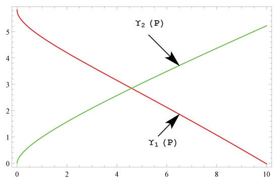
Figure 1. Existence of the unique positive fixed point of System (7).

Suppose that $(H,P)$ be any equilibrium point of System (7), then the Jacobian matrix of System (7) evaluated at equilibrium point $(H,P)$ is given as follows:

$$J(H,P)=\left[\begin{array}{cc}\frac{e^{q{P}^{1-m}}r}{{\left(e^{q{P}^{1-m}}+kH\right)}^2}& -\frac{e^{q{P}^{1-m}}(1-m)qrH{P}^{-m}}{{\left(e^{q{P}^{1-m}}+kH\right)}^2}\\ c\left(1-e^{-q{P}^{1-m}}\right)& cq(1-m)H{e}^{-q{P}^{1-m}}{P}^{-m}\end{array}\right].$$

(10)

Furthermore, about interior fixed point $(H^{*},P^{*})\in \left[0,\frac{r-1}{k}\right]\times \left[0,\frac{c(r-1)}{k}\right]$ of Model (7), the Jacobian matrix $J(H,P)$ given in Equation (10) becomes:

$$J(H^{*},P^{*})=\left[\begin{array}{cc}\frac{exp\left(q{\left(P^{*}\right)}^{1-m}\right)}{r}& -\frac{q(1-m)H^{*}exp\left(q{\left(P^{*}\right)}^{1-m}\right)}{r{\left(P^{*}\right)}^m}\\ c\left(1-exp\left(-q{\left(P^{*}\right)}^{1-m}\right)\right)& \frac{cq(1-m)H^{*}exp\left(-q{\left(P^{*}\right)}^{1-m}\right)}{{\left(P^{*}\right)}^m}\end{array}\right].$$

The following Lemma gives the conditions for local stability of a positive fixed point.

Theorem 3.

The steady-state $(H^{*},P^{*})\in \left[0,\frac{r-1}{k}\right]\times \left[0,\frac{c(r-1)}{k}\right]$ of Model (7) is a sink if the following inequalities are fulfilled:

$${\left(P^{*}\right)}^{m}exp\left(q{\left(P^{*}\right)}^{1-m}\right)+rqc(1-m)H^{*}exp\left(-q{\left(P^{*}\right)}^{1-m}\right)<r{\left(P^{*}\right)}^m+qc(1-m)H^{*}exp\left(q{\left(P^{*}\right)}^{1-m}\right),$$

and

$$qc(1-m)H^{*}exp\left(q{\left(P^{*}\right)}^{1-m}\right)<r{\left(P^{*}\right)}^m.$$

Proof. 

It is easy to compute the characteristic equation for Jacobian matrix $J(H^{*},P^{*})$ as follows

$$\mathbb{P}\left(\lambda \right)={\lambda }^2-TrJ(H^{*},P^{*})\lambda +detJ(H^{*},P^{*}),$$

(11)

where

$$TrJ(H^{*},P^{*})=\frac{exp\left(q{\left(P^{*}\right)}^{1-m}\right)}{r}+\frac{qc(1-m)H^{*}exp\left(-q{\left(P^{*}\right)}^{1-m}\right)}{{\left(P^{*}\right)}^m},$$

and

$$detJ(H^{*},P^{*})=\frac{qc(1-m)H^{*}exp\left(q{\left(P^{*}\right)}^{1-m}\right)}{r{\left(P^{*}\right)}^m}.$$

Arguing as in [31], the roots of Equation (11) lie inside the open unit disk if $\mathbb{P}\left(1\right)>0$, $\mathbb{P}(-1)>0$ and $\mathbb{P}\left(0\right)<1$, that is,

$$\begin{array}{c}{\left(P^{*}\right)}^{m}exp\left(q{\left(P^{*}\right)}^{1-m}\right)+rqc(1-m)H^{*}exp\left(-q{\left(P^{*}\right)}^{1-m}\right)\hfill \\ <r{\left(P^{*}\right)}^m+qc(1-m)H^{*}exp\left(q{\left(P^{*}\right)}^{1-m}\right),\hfill \end{array}$$

(12)

$$\begin{array}{c}{\left(P^{*}\right)}^{m}exp\left(q{\left(P^{*}\right)}^{1-m}\right)+rqc(1-m)H^{*}exp\left(-q{\left(P^{*}\right)}^{1-m}\right)\hfill \\ +r{\left(P^{*}\right)}^m+qc(1-m)H^{*}exp\left(q{\left(P^{*}\right)}^{1-m}\right)>0,\hfill \end{array}$$

(13)

and

$$qc(1-m)H^{*}exp\left(q{\left(P^{*}\right)}^{1-m}\right)<r{\left(P^{*}\right)}^m.$$

(14)

As Inequality (13) is satisfied automatically, the interior fixed point of System (7) is a sink and, thus, asymptotically stable if the Inequalities (12) and (14) are satisfied. □

For $r=2.52$, $c=1.245$, $q=0.286$ and $m=0.194$, a phase analysis for the topological classification of a positive fixed point is depicted in Figure 2.

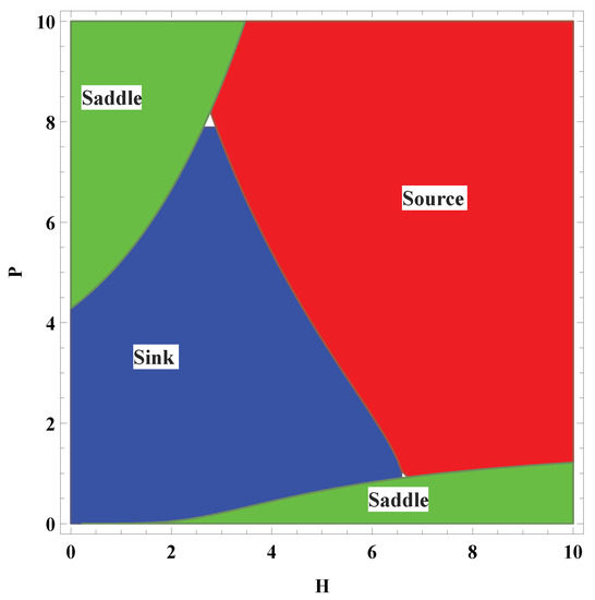
Figure 2. Topological classification for the positive fixed point of System (7).

4. Global Stability

The global stability of the interior fixed point of System (7) is explored in this section.

Arguing as in [32], first of all, the following Lemma is considered.

Lemma 2.

Taking into account some real intervals $I=[a,b]$ and $J=[c,d]$, and assume that $f:I\times J\to I$ and $g:I\times J\to J$ are real-valued continuous functions defined on rectangle $I\times J$. Considering the following system:

$$\begin{array}{c}\hfill \left(\begin{array}{c}{x}_{n+1}\\ y_{n+1}\end{array}\right)=\left(\begin{array}{c}f(x_n,y_n)\\ g(x_n,y_n)\end{array}\right),\end{array}$$

(15)

where $n=0,1,2,\cdots$ and initial conditions $(x_0,y_0)\in I\times J$. Meanwhile, we assume that the following conditions are satisfied:

(i) 

The function $f(x,y)$ is non-decreasing with respect to x, and non-increasing with respect to y.

(ii) 

The function $g(x,y)$ is non-decreasing in both variables x and y.

(iii) 

Assume that $(m_1,M_1,m_2,M_2)\in I^2\times J^2$ solves the following algebraic system:

$$\begin{array}{c}\hfill m_1=f(m_1,M_2),M_1=f(M_1,m_2)\\ \hfill m_2=g(m_1,m_2),M_2=g(M_1,M_2)\end{array}$$

with $m_1=M_1$ and $m_2=M_2$. Then, there exists a fixed point $(x^{*},y^{*})$ for System (15) with satisfying ${\displaystyle \underset{n\to \infty }{lim}(x_n,y_n)=(x^{*},y^{*})}$.

Lemma 3.

Suppose that $0<m<1$ and $r>1$, then interior fixed point of System (7) is a global attractor, if the following inequality holds true:

$$\frac{k}{(1-m)rln\left(r\right)}-cr>0.$$

(16)

Proof. 

Keeping in view the right hand sides of System (7), we consider two real-valued functions

$$f:\left[0,\frac{r-1}{k}\right]\times \left[0,\frac{c(r-1)}{k}\right]\to \left[0,\frac{r-1}{k}\right]$$

and

$$g:\left[0,\frac{r-1}{k}\right]\times \left[0,\frac{c(r-1)}{k}\right]\to \left[0,\frac{c(r-1)}{k}\right]$$

such that $f(x,y):=\frac{rx{e}^{-q{y}^{1-m}}}{1+kx{e}^{-q{y}^{1-m}}}$, and $g(x,y):=cx\left(1-e^{-q{y}^{1-m}}\right)$ with $q,k,c>0$, $0<m<1$ and $r>1$, then the function f is non-decreasing in abscissa and non-increasing in ordinate. On the other hand, g is non-decreasing in both abscissa and ordinate. Assume that $t_1\le T_1$ and $t_2\le T_2$, and $(t_1,T_1,t_2,T_2)\ne (0,0,0,0)$ solves the following system:

$$\begin{array}{c}\hfill t_1=f(t_1,T_2),T_1=f(T_1,t_2),\\ \hfill t_2=g(t_1,t_2),T_2=g(T_1,T_2).\end{array}$$

One can obtain the following systems:

$$\begin{array}{c}\hfill t_1=\frac{r{t}_1{e}^{-q{T}_2^{1-m}}}{1+k{t}_1{e}^{-q{T}_2^{1-m}}},T_1=\frac{r{T}_1{e}^{-q{t}_2^{1-m}}}{1+k{T}_1{e}^{-q{t}_2^{1-m}}},\end{array}$$

(17)

and

$$\begin{array}{c}\hfill t_2=c{t}_1\left(1-e^{-q{t}_2^{1-m}}\right),T_2=c{T}_1\left(1-e^{-q{T}_2^{1-m}}\right).\end{array}$$

(18)

Since $(t_1,T_1)\ne (0,0)$, from Equation (17), we have

$$\begin{array}{c}\hfill e^{q{T}_2^{1-m}}+k{t}_1=r,e^{q{t}_2^{1-m}}+k{T}_1=r.\end{array}$$

(19)

Elimination of r from Equation (19) gives

$$\begin{array}{c}\hfill k(T_1-t_1)=e^{q{T}_2^{1-m}}-e^{q{t}_2^{1-m}}.\end{array}$$

(20)

From Equation (19), we have $e^{q{t}_2^{1-m}}\le e^{q{t}_2^{1-m}}\le r$, and $t_2^{1-m}\le T_2^{1-m}\le \frac{ln\left(r\right)}{q}$. Therefore, from Equation (20), it follows that

$$\begin{array}{cc}\hfill k(T_1-t_1)& =q(1-m)e^{q{\theta }^{1-m}}{\theta }^{-m}(T_2-t_2)\hfill \\ \hfill & \le (1-m)rln\left(r\right)(T_2-t_2),\hfill \end{array}$$

(21)

where $t_2\le \theta \le T_2$. Moreover, subtracting Equation (18), and using Equation (20) with $t_1\le T_1\le \frac{r-1}{k}$ we have

$$\begin{array}{cc}\hfill T_2-t_2& =c(T_1-t_1)+c\left(t_1{e}^{-q{t}_2^{1-m}}-T_1{e}^{-q{T}_2^{1-m}}\right)\hfill \\ \hfill & \le c(T_1-t_1)+c{T}_1\left(e^{-q{t}_2^{1-m}}-e^{-q{T}_2^{1-m}}\right)\hfill \\ \hfill & \le cr(T_1-t_1).\hfill \end{array}$$

(22)

Finally, combining Equations (21) and (22), we have the following inequality

$$\left(\frac{k}{(1-m)rln\left(r\right)}-cr\right)\left(T_1-t_1\right)\le 0.$$

(23)

Suppose that $\frac{k}{(1-m)rln\left(r\right)}-cr>0$, then from Equation (23) we have $t_1=T_1$ and Equation (22) gives $t_2=T_2$. Consequently, Lemma 2 gives confirmation that the interior fixed point of System (7) is a global attractor. □

Theorem 4.

Suppose that $0<m<1$ and $r>1$. In addition, if Equations(12), (14) and (16) are fulfilled, then the interior fixed point of System (7) is globally asymptotically stable.

5. Hopf Bifurcation

This section is dedicated to the existence and direction of Hopf bifurcation about an interior fixed point of System (7).

The roots of Equation (11) are complex conjugate numbers if the following inequality holds true:

$$exp\left(q{\left(P^{*}\right)}^{1-m}\right){\left(P^{*}\right)}^m+qcr(1-m)H^{*}exp\left(-q{\left(P^{*}\right)}^{1-m}\right)<2r{\left(P^{*}\right)}^m.$$

(24)

Suppose that Inequality (24) holds true, then System (7) experiences Hopf bifurcation about its interior fixed point whenever $detJ(H^{*},P^{*}){|}_{c=c_1}=1$, where

$$c_1=\frac{r{\left(P^{*}\right)}^m}{q(1-m)H^{*}exp\left(q{\left(P^{*}\right)}^{1-m}\right)}.$$

(25)

Next, we define a Hopf bifurcation curve ${\mathfrak{S}}_{NB}$ for System (7) as follows:

$${\mathfrak{S}}_{NB}:=\left\{(r,q,m,k,c_1)\in {\mathbb{R}}_{+}^5:detJ(H^{*},P^{*})<2,c_1=\frac{r{\left(P^{*}\right)}^m}{q(1-m)H^{*}exp\left(q{\left(P^{*}\right)}^{1-m}\right)}\right\}.$$

Assume that $(r,q,m,k,c_1)\in {\mathfrak{S}}_{NB}$, and consider

$$\left(\begin{array}{c}H\\ P\end{array}\right)\to \left(\begin{array}{c}\frac{rHexp\left(-q{P}^{1-m}\right)}{1+kHexp\left(-q{P}^{1-m}\right)}\\ c_{1}H\left(1-exp\left(-q{P}^{1-m}\right)\right)\end{array}\right).$$

(26)

Suppose that $\tilde{c}$ indicates a very small perturbation in $c_1$ such that $|\tilde{c}|\ll 1$, and interchanging $c_1$ into $c_1+\tilde{c}$ in Equation (26), we have a perturbed map of the following form:

$$\left(\begin{array}{c}H\\ P\end{array}\right)\to \left(\begin{array}{c}\frac{rHexp\left(-q{P}^{1-m}\right)}{1+kHexp\left(-q{P}^{1-m}\right)}\\ (c_1+\tilde{c})H\left(1-exp\left(-q{P}^{1-m}\right)\right)\end{array}\right).$$

(27)

Further, we suppose that $c_1+\tilde{c}>1$ and $0<m<1$, then positive fixed point of Equation (27) is given by $(H^{*},P^{*})\in \left[0,\frac{r-1}{k}\right]\times \left[0,\frac{(c_1+\tilde{c})(r-1)}{k}\right]$. Focusing on the following translations

$$x=H-H^{*},y=P-P^{*}.$$

(28)

From Equations (27) and (28), it follows that:

$$\left(\begin{array}{c}x\\ y\end{array}\right)\to \left(\begin{array}{cc}{a}_{11}& a_{12}\\ a_{21}& a_{22}\\ \end{array}\right)\left(\begin{array}{c}x\\ y\end{array}\right)+\left(\begin{array}{c}{f}_1(x,y)\\ f_2(x,y)\end{array}\right),$$

(29)

where

$$f_1(x,y)=a_{13}{x}^2+a_{14}xy+a_{15}{y}^2+b_1{x}^3+b_2{x}^{2}y+b_{3}x{y}^2+b_4{y}^3+O\left(\left(\right|x|+{\left|y\right|)}^4\right),$$

$$f_2(x,y)=a_{23}xy+a_{24}{y}^2+d_{1}x{y}^2+d_2{y}^3+O\left(\left(\right|x|+{\left|y\right|)}^4\right),$$

$$a_{11}=\frac{exp\left(q{\left(P^{*}\right)}^{1-m}\right)}{r},a_{12}=-\frac{q(1-m)H^{*}exp\left(q{\left(P^{*}\right)}^{1-m}\right)}{r{\left(P^{*}\right)}^m},$$

$$a_{21}=(c_1+\tilde{c})\left(1-exp\left(-q{\left(P^{*}\right)}^{1-m}\right)\right),a_{22}=\frac{(c_1+\tilde{c})q(1-m)H^{*}exp\left(-q{\left(P^{*}\right)}^{1-m}\right)}{{\left(P^{*}\right)}^m},$$

$$a_{13}=-\frac{kexp\left(q{\left(P^{*}\right)}^{1-m}\right)}{r^2},a_{14}=-\frac{q(1-m)exp\left(q{\left(P^{*}\right)}^{1-m}\right)\left(exp\left(q{\left(P^{*}\right)}^{1-m}\right)-k{H}^{*}\right)}{r^2{\left(P^{*}\right)}^m},$$

$$\begin{array}{cc}\hfill a_{15}& =\frac{q{S}_1}{{\left(P^{*}\right)}^{2m}}\left(H^{*}km-mexp\left(q{\left(P^{*}\right)}^{1-m}\right)-H^{*}k+exp\left(q{\left(P^{*}\right)}^{1-m}\right)\right)\hfill \\ \hfill & +\frac{m{S}_1}{{\left(P^{*}\right)}^{1+m}}\left(k{H}^{*}+exp\left(q{\left(P^{*}\right)}^{1-m}\right)\right),S_1=\frac{H^{*}q(1-m)exp\left(q{\left(P^{*}\right)}^{1-m}\right)}{2r^2},\hfill \end{array}$$

$$b_1=\frac{k^{2}exp\left(q{\left(P^{*}\right)}^{1-m}\right)}{r^3},b_2=\frac{qk(1-m)exp\left(q{\left(P^{*}\right)}^{1-m}\right)\left(2exp\left(q{\left(P^{*}\right)}^{1-m}\right)-k{H}^{*}\right)}{{\left(P^{*}\right)}^m{r}^3},$$

$$\begin{array}{cc}\hfill b_3& =\frac{q(1-m)S_2}{{\left(P^{*}\right)}^{2m}}\left({\left(H^{*}\right)}^2{k}^2-4H^{*}k+exp\left(2q{\left(P^{*}\right)}^{1-m}\right)\right)\hfill \\ \hfill & +\frac{m{S}_2}{{\left(P^{*}\right)}^{1+m}}\left(exp\left(2q{\left(P^{*}\right)}^{1-m}\right)-{\left(H^{*}\right)}^2{k}^2\right),S_2=\frac{q(1-m)exp\left(q{\left(P^{*}\right)}^{1-m}\right)}{2r^3},\hfill \end{array}$$

$$\begin{array}{cc}\hfill b_4& =-\frac{H^{*}{S}_3}{6r}\left({\left(P^{*}\right)}^{-3m}{q}^2{(1-m)}^2-3qm(1-m){\left(P^{*}\right)}^{-1-2m}+m(1+m){\left(P^{*}\right)}^{-2-m}\right)\hfill \\ \hfill & +\frac{H^{*}{S}_3^2}{r^2}\left(q(1-m){\left(P^{*}\right)}^{-3m}-m{\left(P^{*}\right)}^{-1-2m}\right)-\frac{H^{*}{S}_3^3}{r^3},S_3=q(1-m)exp\left(q{\left(P^{*}\right)}^{1-m}\right),\hfill \end{array}$$

$$a_{23}=-(c_1+\tilde{c})q(1-m){\left(P^{*}\right)}^{-m}exp\left(q{\left(P^{*}\right)}^{1-m}\right),$$

$$a_{24}=-\frac{1}{2}(c_1+\tilde{c})H^{*}q(1-m)exp\left(q{\left(P^{*}\right)}^{1-m}\right)\left(q(1-m){\left(P^{*}\right)}^{-2m}-m{\left(P^{*}\right)}^{-1-m}\right),$$

$$d_1=-\frac{1}{2}(c_1+\tilde{c})q(1-m)exp\left(q{\left(P^{*}\right)}^{1-m}\right)\left(q(1-m){\left(P^{*}\right)}^{-2m}-m{\left(P^{*}\right)}^{-1-m}\right),$$

$$d_2=S_4\left(q^2{(1-m)}^2{\left(P^{*}\right)}^{-3m}-3mq(1-m){\left(P^{*}\right)}^{-1-2m}+m(1+m){\left(P^{*}\right)}^{-2-m}\right),$$

$$S_4=-\frac{1}{6}(c_1+\tilde{c})q{H}^{*}(1-m)exp\left(q{\left(P^{*}\right)}^{1-m}\right).$$

Taking into account Equation (29), then the characteristic equation for its variational matrix about $(0,0)$ is of the following form:

$${\lambda }^2-A\left(\tilde{c}\right)\lambda +B\left(\tilde{c}\right)=0,$$

(30)

where

$$A\left(\tilde{c}\right)=\frac{exp\left(q{\left(P^{*}\right)}^{1-m}\right)}{r}+\frac{q(c_1+\tilde{c})(1-m)H^{*}exp\left(-q{\left(P^{*}\right)}^{1-m}\right)}{{\left(P^{*}\right)}^m},$$

and

$$B\left(\tilde{c}\right)=\frac{q(c_1+\tilde{c})(1-m)H^{*}exp\left(q{\left(P^{*}\right)}^{1-m}\right)}{r{\left(P^{*}\right)}^m}.$$

The roots of Equation (30) are given as follows:

$${\lambda }_1,{\lambda }_2=\frac{A\left(\tilde{c}\right)}{2}\pm \frac{i}{2}\sqrt{4B\left(\tilde{c}\right)-A^2\left(\tilde{c}\right)}.$$

On the other hand, we have

$$|{\lambda }_1|=|{\lambda }_2|=\sqrt{B\left(\tilde{c}\right)},$$

and

$${\displaystyle {\left(\frac{d|{\lambda }_1|}{d\tilde{c}}\right)}_{\tilde{c}=0}={\left(\frac{d|{\lambda }_2|}{d\tilde{c}}\right)}_{\tilde{c}=0}=\frac{\sqrt{q(1-m)H^{*}exp\left(q{\left(P^{*}\right)}^{1-m}\right)}}{2\sqrt{c_{1}r{\left(P^{*}\right)}^m}}>0.}$$

Assume that $\tilde{c}=0$, then we have $A\left(0\right)=\frac{exp\left(q{\left(P^{*}\right)}^{1-m}\right)}{r}+\frac{q{c}_1(1-m)H^{*}exp\left(-q{\left(P^{*}\right)}^{1-m}\right)}{{\left(P^{*}\right)}^m}>0$ and $A\left(0\right)<2$ because $(r,q,m,k,c_1)\in {\mathfrak{S}}_{NB}$. Consequently, one has $A\left(0\right)\ne \pm 2,0,-1$ gives ${\lambda }_1^n,{\lambda }_2^n\ne 1$ at $\tilde{c}=0$ for all $n=1,2,3,4$. Consequently, the roots of Equation (30) do not meet the unit circle at $\tilde{c}=0$. Next, we suppose that $\alpha =\frac{A\left(0\right)}{2}$ and $\beta =\frac{1}{2}\sqrt{4B\left(0\right)-A^2\left(0\right)}$ and considering a transformation of the following form:

$$\left(\begin{array}{c}x\\ y\end{array}\right)=\left(\begin{array}{cc}-\frac{q(1-m)H^{*}exp\left(q{\left(P^{*}\right)}^{1-m}\right)}{r{\left(P^{*}\right)}^m}& 0\\ \alpha -\frac{exp\left(q{\left(P^{*}\right)}^{1-m}\right)}{r}& -\beta \\ \end{array}\right)\left(\begin{array}{c}u\\ v\end{array}\right).$$

(31)

From Equations (29) and (31), one has

$$\left(\begin{array}{c}u\\ v\end{array}\right)\to \left(\begin{array}{cc}\alpha & -\beta \\ \beta & \alpha \\ \end{array}\right)\left(\begin{array}{c}u\\ v\end{array}\right)+\left(\begin{array}{c}\tilde{f}(u,v)\\ \tilde{g}(u,v)\end{array}\right),$$

(32)

where

$$\tilde{f}(u,v)=\frac{a_{13}}{a_{12}}{x}^2+\frac{a_{14}}{a_{12}}xy+\frac{a_{15}}{a_{12}}{y}^2+\frac{b_1}{a_{12}}{x}^3+\frac{b_2}{a_{12}}{x}^{2}y+\frac{b_3}{a_{12}}x{y}^2+\frac{b_4}{a_{12}}{y}^3+O\left(\left(\right|u|+{\left|v\right|)}^4\right),$$

$$\begin{array}{ccc}\hfill \tilde{g}(u,v)& =& \frac{a_{13}(\alpha -a_{11})}{\beta a_{12}}{x}^2+\left(\frac{a_{14}(\alpha -a_{11})}{\beta a_{12}}-\frac{a_{23}}{\beta }\right)xy+\left(\frac{a_{15}(\alpha -a_{11})}{\beta a_{12}}-\frac{a_{24}}{\beta }\right)y^2\hfill \\ & +& \frac{b_1(\alpha -a_{11})}{\beta a_{12}}{x}^3+\frac{b_2(\alpha -a_{11})}{\beta a_{12}}{x}^{2}y+\left(\frac{b_3(\alpha -a_{11})}{\beta a_{12}}-\frac{d_1}{\beta }\right)x{y}^2\hfill \\ & +& \left(\frac{b_4(\alpha -a_{11})}{\beta a_{12}}-\frac{d_2}{\beta }\right)y^3+O\left(\left(\right|u|+{\left|v\right|)}^4\right),\hfill \end{array}$$

$x=a_{12}u$ and $y=(\alpha -a_{11})u-\beta v$. Next, we consider the following first Lyapunov exponent:

$$L={\left(\left[-Re\left(\frac{(1-2{\lambda }_1){\lambda }_2^2}{1-{\lambda }_1}{\xi }_{20}{\xi }_{11}\right)-\frac{1}{2}|{\xi }_{11}{|}^2-{\left|{\xi }_{02}\right|}^2+Re\left({\lambda }_2{\xi }_{21}\right)\right]\right)}_{\tilde{r}=0},$$

where

$${\xi }_{20}=\frac{1}{8}\left[{\tilde{f}}_{uu}-{\tilde{f}}_{vv}+2{\tilde{g}}_{uv}+i\left({\tilde{g}}_{uu}-{\tilde{g}}_{vv}-2{\tilde{f}}_{uv}\right)\right],$$

$${\xi }_{11}=\frac{1}{4}\left[{\tilde{f}}_{uu}+{\tilde{f}}_{vv}+i\left({\tilde{g}}_{uu}+{\tilde{g}}_{vv}\right)\right],$$

$${\xi }_{02}=\frac{1}{8}\left[{\tilde{f}}_{uu}-{\tilde{f}}_{vv}-2{\tilde{g}}_{uv}+i\left({\tilde{g}}_{uu}-{\tilde{g}}_{vv}+2{\tilde{f}}_{uv}\right)\right],$$

$${\xi }_{21}=\frac{1}{16}\left[{\tilde{f}}_{uuu}+{\tilde{f}}_{uvv}+{\tilde{g}}_{uuv}+{\tilde{g}}_{vvv}+i\left({\tilde{g}}_{uuu}+{\tilde{g}}_{uvv}-{\tilde{f}}_{uuv}-{\tilde{f}}_{vvv}\right)\right].$$

Keeping in view the above calculations and normal form theory of bifurcation [33,34,35,36], we have the following result:

Theorem 5.

Assuming that $L\ne 0$, then Model (7) experiences Hopf bifurcation around its interior fixed point denoted by $(H^{*},P^{*})$ whenever c deviates in small locality of

$$c_1=\frac{r{\left(P^{*}\right)}^m}{q(1-m)H^{*}exp\left(q{\left(P^{*}\right)}^{1-m}\right)}.$$

In addition, if $L<0$, then a closed invariant curve of attracting nature bifurcates from the positive fixed point towards $c>c_1$, on the other hand, if $L>0$, then a repelling invariant closed curve bifurcates from the fixed point towards $c<c_1$.

6. Chaos and Bifurcation Control

Control of bifurcation and chaos is a topic of great interest. Particularly, chaos and bifurcation control methods are more applicable for models of discrete nature because such system are of complex behavior as compare to continuous ones. On the other hand, chaos control methods are widely used in almost all branches of applied science [37]. For further details related to chaos control methods in discrete-time systems, we refer to [38,39,40,41,42,43,44,45,46,47,48].

In this section, we discuss two chaos control methods for System (7). The first method is a modification of the Ott-Grebogi-Yorke (OGY) method [49], known as the pole-placement method [50]. For the application of the pole-placement method to Model (7), we rewrite this system as follows:

$$\begin{array}{cc}\hfill H_{n+1}& =\frac{r{H}_{n}exp\left(-q{P}_n^{1-m}\right)}{1+k{H}_{n}exp\left(-q{P}_n^{1-m}\right)}=f\left(H_n,P_n,c\right)\hfill \\ \hfill P_{n+1}& =c{H}_n\left(1-exp\left(-q{P}_n^{1-m}\right)\right)=g\left(H_n,P_n,c\right),\hfill \end{array}$$

(33)

where c is used for the sake of the control parameter. On the other hand, it is assumed that control parameter c satisfies $|c-c_0|<\delta$, where $\delta >0$ and $c_0$ represents some nominal value, which is located in the chaotic or bifurcating region. Next, we suppose that $\left(H^{*},P^{*}\right)$ is an interior unstable fixed point of System (7). Furthermore, it is also assumed that $\left(H^{*},P^{*}\right)$ is located in some chaotic region. Our main target is to move the unstable fixed point towards a stable one. For this, System (33) is linearized about the an unstable fixed point $\left(H^{*},P^{*}\right)$ as follows:

$$\left[\begin{array}{c}{H}_{n+1}-H^{*}\\ P_{n+1}-P^{*}\end{array}\right]\approx A\left[\begin{array}{c}{H}_n-H^{*}\\ P_n-P^{*}\end{array}\right]+B[c-c_0],$$

(34)

where

$$A=\left[\begin{array}{cc}\frac{\partial f\left(H^{*},P^{*},c_0\right)}{\partial H_n}& \frac{\partial f\left(H^{*},P^{*},c_0\right)}{\partial P_n}\\ \frac{\partial g\left(H^{*},P^{*},c_0\right)}{\partial H_n}& \frac{\partial g\left(H^{*},P^{*},c_0\right)}{\partial P_n}\end{array}\right],B=\left[\begin{array}{c}\frac{\partial f\left(H^{*},P^{*},c_0\right)}{\partial c}\\ \frac{\partial g\left(H^{*},P^{*},c_0\right)}{\partial c}\end{array}\right]=\left[\begin{array}{c}0\\ H^{*}\left(1-exp\left(-q{\left(P^{*}\right)}^{1-m}\right)\right)\end{array}\right].$$

Next, we define the following controllability matrix for System (33):

$$C=\left[B:AB\right]=\left[\begin{array}{cc}0& \left(\frac{\partial f\left(H^{*},P^{*},c_0\right)}{\partial P_n}\right)\left(H^{*}\left(1-exp\left(-q{\left(P^{*}\right)}^{1-m}\right)\right)\right)\\ H^{*}\left(1-exp\left(-q{\left(P^{*}\right)}^{1-m}\right)\right)& \left(\frac{\partial g\left(H^{*},P^{*},c_0\right)}{\partial P_n}\right)\left(H^{*}\left(1-exp\left(-q{\left(P^{*}\right)}^{1-m}\right)\right)\right)\end{array}\right].$$

(35)

Then, it is easy to see that rank matrix C is two. Indeed, $H^{*}\left(1-exp\left(-q{\left(P^{*}\right)}^{1-m}\right)\right)\ne 0$; thus, the system is controllable. Furthermore, in order to apply the pole-placement method, we consider that $[c-c_0]=-K\left[\begin{array}{c}{H}_n-H^{*}\\ P_n-P^{*}\end{array}\right]$, where $K=\left[\begin{array}{cc}{k}_1& k_2\end{array}\right]$. Consequently, System (34) takes the following form:

$$\left[\begin{array}{c}{H}_{n+1}-H^{*}\\ P_{n+1}-P^{*}\end{array}\right]\approx \left[A-BK\right]\left[\begin{array}{c}{H}_n-H^{*}\\ P_n-P^{*}\end{array}\right].$$

(36)

On the other hand, fixed point $\left(H^{*},P^{*}\right)$ is asymptotically stable provided that the multipliers for the variational matrix $A-BK$ lie inside the open unit disk. Assume that ${\mu }_1$ and ${\mu }_2$ are multipliers of variational matrix $A-BK$. In addition, we take ${\lambda }^2+{\alpha }_1\lambda +{\alpha }_2=0$ as a characteristic polynomial for matrix A and ${\mu }^2+{\beta }_1\mu +{\beta }_2=0$ is taken as a characteristic polynomial for $A-BK$. Then, a unique solution of the pole-placement method is provided as follows:

$$K=\left[\begin{array}{cc}{\beta }_2-{\alpha }_2& {\beta }_1-{\alpha }_1\end{array}\right]T^{-1},$$

(37)

where $T=CM$ and $M=\left[\begin{array}{cc}{\alpha }_1& 1\\ 1& 0\end{array}\right]$. Due to some simple computation, one has

$$T=CM=\left[\begin{array}{cc}\frac{\partial f}{\partial P_n}\frac{\partial g}{\partial c}& 0\\ {\alpha }_1\frac{\partial g}{\partial c}+\frac{\partial g}{\partial P_n}\frac{\partial g}{\partial c}& \frac{\partial g}{\partial c}\end{array}\right],$$

(38)

here, all these partial derivatives are calculated at $(H^{*},P^{*},c_0)$. Next, from Equations (37) and (38), it follows that:

$$k_1=\frac{{\beta }_2-{\alpha }_2}{\left(\frac{\partial f(H^{*},P^{*},c_0)}{\partial P_n}\right)\left(\frac{\partial g(H^{*},P^{*},c_0)}{\partial c}\right)}-\frac{({\beta }_1-{\alpha }_1)\left({\alpha }_1+\frac{\partial g(H^{*},P^{*},c_0)}{\partial P_n}\right)}{\left(\frac{\partial f(H^{*},P^{*},c_0)}{\partial P_n}\right)\left(\frac{\partial g(H^{*},P^{*},c_0)}{\partial c}\right)},k_2=\frac{{\beta }_1-{\alpha }_1}{\frac{\partial g(H^{*},P^{*},c_0)}{\partial c}}.$$

Secondly, the hybrid control method [51] is applied to System (7). For this, the controlled system related to System (7) is written in the following form:

$$\begin{array}{cc}\hfill H_{n+1}& =\alpha \frac{r{H}_{n}exp\left(-q{P}_n^{1-m}\right)}{1+k{H}_{n}exp\left(-q{P}_n^{1-m}\right)}+(1-\alpha )H_n\hfill \\ \hfill P_{n+1}& =\alpha c{H}_n\left(1-exp\left(-q{P}_n^{1-m}\right)\right)+(1-\alpha )P_n,\hfill \end{array}$$

(39)

Then, a variational matrix for System (39) about a positive fixed point $(H^{*},P^{*})$ is given as follows:

$${\displaystyle \left[\begin{array}{cc}1-\alpha +\frac{\alpha }{r}{e}^{q{\left(P^{*}\right)}^{1-m}}& -\frac{\alpha (1-m)q{H}^{*}{e}^{q{\left(P^{*}\right)}^{1-m}}}{r{\left(P^{*}\right)}^m}\\ \alpha c\left(1-e^{-q{\left(P^{*}\right)}^{1-m}}\right)& \alpha c(1-m)q{H}^{*}{e}^{-q{\left(P^{*}\right)}^{1-m}}{\left(P^{*}\right)}^{-m}+1-\alpha \end{array}\right].}$$

(40)

For controllability of System (39) about its positive fixed point, the following result is presented:

Lemma 4.

The positive steady-state $(H^{*},P^{*})$ for System (39) is controllable, if the following inequalities are satisfied:

$$e^{q{\left(P^{*}\right)}^{1-m}}+rc(1-m)q{H}^{*}{e}^{-q{\left(P^{*}\right)}^{1-m}}{\left(P^{*}\right)}^{-m}<r+c(1-m)q{H}^{*}{e}^{q{\left(P^{*}\right)}^{1-m}}{\left(P^{*}\right)}^{-m},$$

and

$$(1-\alpha )\left(1-\alpha +\frac{\alpha }{r}{e}^{q{\left(P^{*}\right)}^{1-m}}\right)+\alpha c(1-m)q{H}^{*}{\left(P^{*}\right)}^{-m}\left((1-\alpha )e^{-q{\left(P^{*}\right)}^{1-m}}+\frac{\alpha }{r}{e}^{q{\left(P^{*}\right)}^{1-m}}\right)<1.$$

7. Numerical Simulations and Discussion

This section is dedicated to the numerical verification of our theoretical discussion. For plots related to phase portraits, bifurcation diagrams and maximum Lyapunov exponents, Mathematica and Matlab are used.

Example 1.

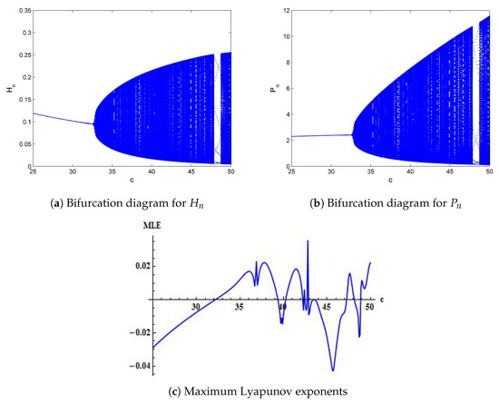
For the verification of Hopf bifurcation about a positive steady-state of System (7), we choose $(r,q,m,k)=(5.4,0.9,0.4,8.3)$ and initial conditions are taken as $(H_0,P_0)=(0.0952,2.416)$. Furthermore, we assume that bifurcation parameter $c\in [25,50]$, then System (7) goes through Hopf bifurcation at $c\approx 32.49$. Then, corresponding diagrams for bifurcation and maximum Lyapunov exponents (MLE) are shown in Figure 3. On the other hand, for $(r,q,m,k,c)=(5.4,0.9,0.4,8.3,32.49)$, System (7) possesses a positive fixed point, which is given by $(H^{*},P^{*})=(0.095015,2.41759735)$, and characteristic polynomial for variational matrix about $(H^{*},P^{*})=(0.095015,2.41759735)$ is computed as follows:

$${\lambda }^2-1.1079103584517793\lambda +1=0.$$

(41)

Figure 3. Bifurcation diagrams and maximum Lyapunov exponents (MLE) for System (7) with (r, q, m, k) = (5.4, 0.9, 0.4, 8.3), (H₀, P₀) = (0.0952, 2.416) and $c\in [25,50]$

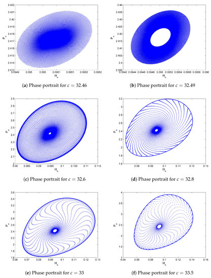
It is easy to see that the roots of Equation (41) are given by ${\lambda }_{1,2}=0.5539551792258897\pm 0.8325464908392879i$ such that $|{\lambda }_{1,2}|=1$. Consequently, $(r,q,m,k,c)=(5.4,0.9,0.4,8.3,32.49)\in {\mathfrak{S}}_{NB}$. Moreover, some phase portraits for System (7) are depicted in Figure 4.

Figure 4. Phase portraits of System (7) for different values of c with (r, q, m, k) = (5.4, 0.9, 0.4, 8.3) and initial conditions (H₀, P₀) = (0.0952, 2.416).

Example 2.

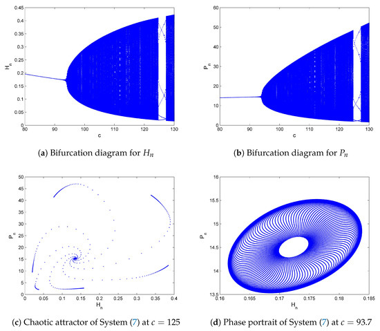
Now, we discuss the affectivity of chaos control methods. First, we implement the pole-placement method. For this, let us consider that $r=12.5$, $q=0.6$, $m=0.5$, $k=15.5$, and $80\le c\le 130$, then Model (7) goes through Hopf bifurcation when $c\approx 93.7$ (cf. Figure 5d). The diagrams for bifurcation of System (7) are shown in Figure 5 (see Figure 5a,b). Furthermore, Figure 5c reveals that an invariant closed curve vanishes at $c=125$ and, consequently, a chaotic orbit appears. Next, choosing $(r,q,m,k,c)=(12.5,0.6,0.5,15.5,125)$. For these selected parameters, System (7) possesses a positive fixed point $(0.13491760154988774,15.244461821003831)$, which is unstable because, for these parametric values, the characteristic polynomial for variational matrix of Equation (7) about $(H^{*},P^{*})=(0.13491760154988774,15.244461821003831)$ is of the following form:

$${\lambda }^2-0.9571949410778701\lambda +1.0790300259105057=0.$$

(42)

Then, one can easily compute the roots of Equation (42), which are given by ${\lambda }_{1,2}=0.478597471\pm 0.92194061i$ and further calculation yields that $|{\lambda }_{1,2}|=1.03876>1$. Here, we select $c_0=125$ as the nominal value in the chaotic region for the following controlled system:

$$\begin{array}{cc}\hfill H_{n+1}& =\frac{12.5H_{n}exp\left(-0.6\sqrt{P_n}\right)}{1+15.5H_{n}exp\left(-0.6\sqrt{P_n}\right)},\hfill \\ \hfill P_{n+1}& =\left(125-k_1(H_n-H^{*})-k_2(P_n-P^{*})\right)H_n\left(1-exp\left(-0.6\sqrt{P_n}\right)\right),\hfill \end{array}$$

(43)

where $(H^{*},P^{*})$ is positive fixed point of Equation (43) and given by $(H^{*},P^{*})=(0.1349176,15.244461821)$. Furthermore, one has the following matrices:

$$A=\left[\begin{array}{cc}0.8327021740781393& -0.00863224020728405\\ 112.99090441781215& 0.124492766999731\end{array}\right],B=\left[\begin{array}{c}0\\ 0.12195569456803064\end{array}\right]$$

and $C=\left[\begin{array}{cc}0& -0.0010527508501574072\\ 0.12195569456803064& 0.015182601868148198\end{array}\right]$ is a matrix with rank 2. Therefore, it is easy to see that System (43) is controllable. Furthermore, we choose $K=\left[\begin{array}{cc}{k}_1& k_2\end{array}\right]$. On the other hand, the variational matrix for System (43) is computed as follows:

$$A-BK=\left[\begin{array}{cc}0.832702& -0.00863224\\ 112.991-0.121956k_1& 0.124493-0.121956k_2\end{array}\right].$$

With some simple calculation, one can easily find characteristic polynomial for matrix $A-BK$ in the following:

$${\lambda }^2-\left(0.957195-0.121956k_2\right)\lambda +1.07903-0.00105275k_1-0.101553k_2=0.$$

(44)

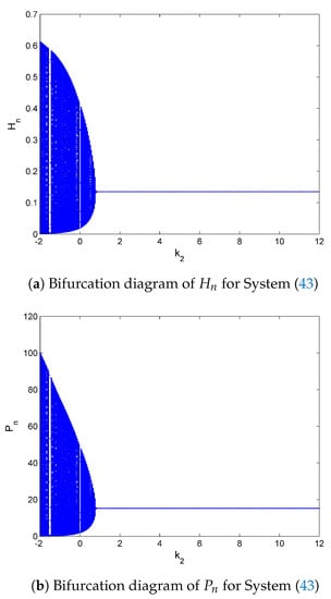
Calculations performing with Mathematica yields that the roots of Equation (44) lie inside the unit open disk if and only if $0.00471012k_1+k_2<13.5844$, $-2264<k_1\le 899.905$ and $0.0103665k_1+k_2>0.778216$, or $899.905<k_1<1217.74$ and $0.051598k_1<54.984+k_2$. Next, if we choose $k_1=1$, then it is easy to see that the roots of Equation (44) lie inside the unit open disk if and only if $0.76785<k_2<13.5797$. With choosing $k_1=1$ and $k_2$ as the bifurcation parameter for System (43) such that $k_2\in \left[-2,12\right]$, then System (43) goes through Hopf bifurcation. The diagrams for bifurcation for System (43) are depicted in Figure 6.

Figure 5. Bifurcation diagrams and phase portraits for System (7) with (r, q, m, k) = (12.5, 0.6, 0.5, 15.5), and $c\in [80,130]$.

Figure 6. Bifurcation diagrams for the controlled System (43) with k1 = ₁, k₂ $\in [-2,12]$ and initial conditions (H₀, P₀) = (0.13, 15).

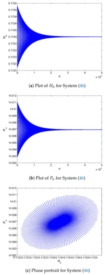
Secondly, we apply the hybrid control method. For this, let us consider $r=12.5$, $q=0.6$, $m=0.5$, $k=15.5$, and $c=93.7$, then System (7) possesses a positive fixed point which is given by $(0.17236,14.50693)$ and characteristic polynomial for variational matrix of (7) about fixed point $(0.17236,14.50693)$ is computed as follows:

$${\lambda }^2-0.9157008538239737\lambda +1=0.$$

(45)

A simple calculation yields that the roots of Equation (45) are of the form ${\lambda }_{1,2}=0.45785042691198685\pm 0.889029238313629i$ with their absolute values $|{\lambda }_{1,2}|=1$. In this case, System (39) can be rewritten as follows:

$$\begin{array}{cc}\hfill H_{n+1}& =\frac{12.5\alpha H_{n}exp\left(-0.6\sqrt{P_n}\right)}{1+15.5H_{n}exp\left(-0.6\sqrt{P_n}\right)}+(1-\alpha )H_n,\hfill \\ \hfill P_{n+1}& =93.7\alpha H_n\left(1-exp\left(-0.6\sqrt{P_n}\right)\right)+(1-\alpha )P_n.\hfill \end{array}$$

(46)

It is easy to see that System (46) possesses a positive fixed point $(H_{*},P_{*})=(0.17236,14.50693)$. On the other hand, the variational matrix for Equation (46) around $(0.17236,14.50693)$ is computed as follows:

$$\left[\begin{array}{cc}1-0.213727\alpha & -0.0106744\alpha \\ 84.1664\alpha & 1-0.870573\alpha \end{array}\right].$$

(47)

Furthermore, one can simply find characteristic polynomial for Equation (47) as follows:

$${\lambda }^2-\left(2-1.0843\alpha \right)\lambda +1-1.0843\alpha +1.08449{\alpha }^2=0.$$

(48)

An application of Jury condition gives that roots of Equation (48) lie inside the open unit disk iff $0<\alpha <0.999823$. Therefore, Hopf bifurcation is almost eliminated completely. Next, choosing $\alpha =0.9995$ plots for System (46) are shown in Figure 7. These plots reveal that the positive fixed point $(0.17236,14.50693)$ of System (46) is a sink (see Figure 7a–c).

Figure 7. Plots for the controlled System (46) with α = 0.9995 and initial conditions (H₀, P₀) = (0.1724, 14.51).

Example 3.

In the end, we take $r=4.75$, $q=0.99$, $m=0.95$, $k=5.5$ and $c=3.1$, then System (7) possesses a unique positive steady-state $(H^{*},P^{*})=(0.3816089836378311,0.7367710807002495)$. Moreover, for these selected values, the characteristic equation of the System (7) about fixed point $(H^{*},P^{*})=(0.3816089836378311,0.7367710807002495)$ is given as follows:

$${\lambda }^2-0.5876616425180492\lambda +0.043687815358447304=0.$$

(49)

The real distinct roots of characteristic Equation (49) are given by:

$${\lambda }_1=0.08731511686028993,{\lambda }_2=0.5003465256577593.$$

Obviously, $|{\lambda }_1|<|{\lambda }_2|<1$. Consequently, the positive steady-state for System (7) is a sink. On the other hand, in order to discuss the global asymptotic stability of the system about this fixed point, one can easily verify Condition (16) of Lemma 3 as follows:

$$\frac{k}{(1-m)rln\left(r\right)}-cr=0.13748097167976425>0.$$

(50)

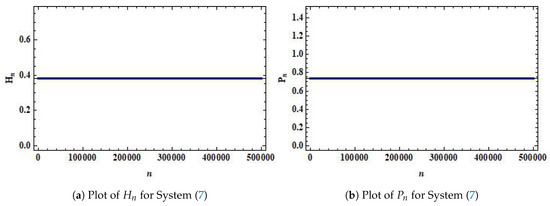
Condition (50) shows that the unique positive equilibrium point $(H^{*},P^{*})=(0.38161,0.73677)$ is globally asymptotically stable. In order to verify this fact numerically, we choose $r=4.75$, $q=0.99$, $m=0.95$, $k=5.5$ and $c=3.1$ with initial conditions $(H_0,P_0)=(8\times {10}^{10},5\times {10}^{10})$, which are far away from the neighborhood of the equilibrium point $(H^{*},P^{*})=(0.38161,0.73677)$, but Figure 8 shows that the equilibrium point $(H^{*},P^{*})=(0.38161,0.73677)$ is globally asymptotically stable.

Figure 8. Plots for System (7) with r = 4.75, q = 0.99, m = 0.95, k = 5.5, c = 3.1 and initial conditions (H₀, P₀) = (8 × 10¹⁰, 5 × 10¹⁰).

8. Concluding Remarks

This paper is concerned with the investigation of some qualitative aspects of a host-parasitoid model. The model is a modification of a generalized Hassell-Varley model of a host-parasitoid system, which can be useful for the description of ecosystems. In addition, the host-parasitoid interactions in which the growth of the host is governed by the Beverton-Holt law have been studied. These findings reveal that the quest constant and mutual interference of parasitoid interaction can be sources for stabilization or destabilization factors for this interaction. On the other hand, restrained interference can assist coexistence between the parasitoid and the host. Meanwhile, this study reveals that the reproductive rate of the parasitoid and the proceeding population growth can also produce a strong destabilization factor, resulting in a variety of complexities and chaotic behavior. Our mathematical findings include the persistence of solutions with the implementation of a method of comparison. Moreover, the existence and uniqueness of an interior fixed point along its local stability analysis are carried out. It is proved that an interior fixed point of the system is globally asymptotically stable. On the other hand, the host-parasitoid model undergoes Neimark-Sacker bifurcation around its interior fixed point. Two chaos control methods are applied for the control of bifurcating and the chaotic behavior of the system. Our investigation reveals that the pole-placement method and hybrid control strategy both are effective for the stability of corresponding controlled systems. In order to validate the proposed generalized Hassell-Varley Model (7) with real data based on statistical analysis using both field and experimental data, the parametric values for System (7) are estimated in Table 1. Keeping in view the estimated parametric value in Table 1, it is easy to see that the positive equilibrium of System (7) is a sink for $20\le c<54.128$. Moreover, System (7) undergoes Neimark-Sacker bifurcation at its positive steady-state as bifurcation parameter c passes through a critical value $c\approx 54.128$. The bifurcation diagrams and phase portrait of System (7) are depicted in Figure 9. Consequently, our theoretical investigations show an excellent validation of field and experimental data.

Table 1. Estimation for values of the parameters.

ine Parameter	Description	Observed Value	Source
ineine r	Host maximum population growth rate	40	[27]
ine k	Host steady population size	0.09	[27]
ine q	Quest constant	0.1	[30]
ine m	Mutual interference constant	0.6	[30]
ine c	Intrinsic growth rate of parasitoid	$20\le c\le 100$	Estimate
ine

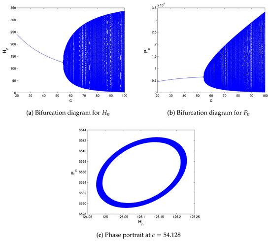
Figure 9. Bifurcation diagrams and phase portrait of System (7) with respect to estimated values.

9. Future Problems

It is interesting to work on bifurcation analysis of the models presented in [52,53,54,55].

References

- Zhang, X.; Zhang, Q.L.; Sreeram, V. Bifurcation analysis and control of a discrete harvested prey-predator system with Beddington-DeAngelis functional response. J. Franklin Inst. 2010, 347, 1076–1096. [Google Scholar] [CrossRef]
- Taylor, A.D. Parasitiod competition and the dynamics of host-parasitoid models. Am. Nat. 1988, 132, 417–436. [Google Scholar] [CrossRef]
- Kaitala, V.; Ylikarjula, J.; Heino, M. Dynamic complexities in host-parasitoid interaction. J. Theor. Biol. 1999, 197, 331–341. [Google Scholar] [CrossRef]
- Tang, S.Y.; Chen, L.S. Chaos in functional response host-parasitoid ecosystem models. Chaos Soliton Fract. 2002, 13, 875–884. [Google Scholar] [CrossRef]
- Xu, C.L.; Boyce, M.S. Dynamic complexities in a mutual interference host-parasitoid model. Chaos Soliton Fract. 2005, 24, 175–182. [Google Scholar] [CrossRef]
- Lv, S.J.; Zhao, M. The dynamic complexity of a host-parasitoid model with a lower bound for the host. Chaos Soliton Fract. 2008, 36, 911–919. [Google Scholar] [CrossRef]
- Din, Q. Global behavior of a plant-herbivore model. Adv. Differ. Equ. 2015, 2015, 119. [Google Scholar] [CrossRef]
- Din, Q. Global behavior of a host-parasitoid model under the constant refuge effect. Appl. Math. Model. 2016, 40, 2815–2826. [Google Scholar] [CrossRef]
- Din, Q.Ö.; Gümüş, A.; Khalil, H. Neimark-Sacker bifurcation and chaotic behaviour of a modified host-parasitoid model. Z. Naturforsch. A 2017, 72, 25–37. [Google Scholar] [CrossRef]
- Din, Q. Global stability and Neimark-Sacker bifurcation of a host-parasitoid model. Int. J. Syst. Sci. 2017, 48, 1194–1202. [Google Scholar] [CrossRef]
- Din, Q. Neimark-Sacker bifurcation and chaos control in Hassell-Varley model. J. Differ. Equ. Appl. 2017, 23, 741–762. [Google Scholar] [CrossRef]
- Din, Q. Global stability of Beddington model. Qual. Theor. Dyn. Syst. 2017, 16, 391–415. [Google Scholar] [CrossRef]
- Din, Q.; Khan, M.A.; Saeed, U. Qualitative Behaviour of Generalised Beddington Model. Z. Naturforsch. A 2016, 71, 145–155. [Google Scholar] [CrossRef]
- Din, Q. Qualitative analysis and chaos control in a density-dependent host-parasitoid system. Int. J. Dyn. Control 2018, 6, 778–798. [Google Scholar] [CrossRef]
- Din, Q.; Hussain, M. Controlling chaos and Neimark-Sacker bifurcation in a host-parasitoid model. Asian J. Control 2019, 21, 1202–1215. [Google Scholar] [CrossRef]
- Wu, D.; Zhao, H. Global qualitative analysis of a discrete host-parasitoid model with refuge and strong Allee effects. Math. Method. Appl. Sci. 2018, 41, 2039–2062. [Google Scholar] [CrossRef]
- Jamieson, W.T. On the global behaviour of May’s host-parasitoid model. J. Differ. Equ. Appl. 2019, 25, 583–596. [Google Scholar] [CrossRef]
- Liu, H.; Zhang, K.; Ye, Y.; Wei, Y.; Ma, M. Dynamic complexity and bifurcation analysis of a host-parasitoid model with Allee effect and Holling type III functional response. Adv. Differ. Equ. 2019, 2019, 507. [Google Scholar] [CrossRef]
- Liu, X.; Chu, Y.; Liu, Y. Bifurcation and chaos in a host-parasitoid model with a lower bound for the host. Adv. Differ. Equ. 2018, 2018, 31. [Google Scholar] [CrossRef]
- Bešo, E.; Kalabušić, E.; Mujić, N.; Pilav, E. Neimark-Sacker bifurcation and stability of a certain class of a host-parasitoid models with a host refuge effect. Int. J. Bifurcat. Chaos 2019, 29, 195169. [Google Scholar]
- Bešo, E.; Mujić, N.; Kalabušić, S.; Pilav, E. Stability of a certain class of a host-parasitoid models with a spatial refuge effect. J. Biol. Dyn. 2020, 14, 1–31. [Google Scholar]
- Alba-Pérez, J.; Macias-Diaz, J.E. Analysis of structure-preserving discrete models for predator-prey systems with anomalous diffusion. Mathematics 2019, 7, 1172. [Google Scholar] [CrossRef]
- Suryanto, A.; Darti, I.; Panigoro, H.S.; Kilicman, A. A fractional-order predator-prey model with ratio-dependent functional response and linear harvesting. Mathematics 2019, 7, 1100. [Google Scholar] [CrossRef]
- Zhang, J.; Zhang, L.; Bai, Y. Stability and bifurcation analysis on a predator-prey system with the weak Allee effect. Mathematics 2019, 7, 432. [Google Scholar] [CrossRef]
- Bailey, V.A.; Nicholson, A.J. The balance of animal populations. Proc. Zool. Soc. Lond. 1935, 3, 551–598. [Google Scholar]
- Ricker, W.E. Stock and recruitment. J. Fish. Res. Board Can. 1954, 11, 559–623. [Google Scholar] [CrossRef]
- Hassell, M.P. Density—Dependence in single—Species populations. J. Anim. Ecol. 1975, 44, 283–295. [Google Scholar] [CrossRef]
- Beverton, R.J.H.; Holt, S.J. On the Dynamics of Exploited Fish Populations; Springer: Dordrecht, The Netherlands, 1993. [Google Scholar]
- Misra, J.C.; Mitra, A. Instabilities in single-species and host-parasite systems: Period-doubling bifurcations and chaos. Comput. Math. Appl. 2006, 52, 525–538. [Google Scholar] [CrossRef]
- Hassell, M.P.; Varley, G.C. New inductive population model for insect parasites and its bearing on biological control. Nature 1969, 223, 1133–1137. [Google Scholar] [CrossRef]
- Liu, X.; Xiao, D. Complex dynamic behaviors of a discrete-time predator-prey system. Chaos Soliton Fract. 2007, 32, 80–94. [Google Scholar] [CrossRef]
- Grove, E.A.; Ladas, G. Periodicities in Nonlinear Difference Equations; Chapman and Hall/CRC Press: Boca Raton, FL, USA, 2004. [Google Scholar]
- Guckenheimer, J.; Holmes, P. Nonlinear Oscillations, Dynamical Systems, and Bifurcations of Vector Fields; Springer: New York, NY, USA, 1983. [Google Scholar]
- Robinson, C. Dynamical Systems: Stability, Symbolic Dynamics and Chaos; Taylor Francis Group: Boca Raton, NY, USA, 1999. [Google Scholar]
- Wiggins, S. Introduction to Applied Nonlinear Dynamical Systems and Chaos; Springer: New York, NY, USA, 2003. [Google Scholar]
- Wan, Y.H. Computation of the stability condition for the Hopf bifurcation of diffeomorphism on R2. SIAM J. Appl. Math. 1978, 34, 167–175. [Google Scholar] [CrossRef]
- Lynch, S. Dynamical Systems with Applications Using Mathematica; Birkhäuser: Boston, MA, USA, 2007. [Google Scholar]
- Din, Q. Complexity and chaos control in a discrete-time prey-predator model. Commun. Nonlinear Sci. Numer. Simul. 2017, 49, 113–134. [Google Scholar] [CrossRef]
- Din, Q. Bifurcation analysis and chaos control in discrete-time glycolysis models. J. Math. Chem. 2018, 56, 904–931. [Google Scholar] [CrossRef]
- Din, Q.; Donchev, T.; Kolev, D. Stability, Bifurcation Analysis and Chaos Control in Chlorine Dioxide-Iodine-Malonic Acid Reaction. MATCH Commun. Math. Comput. Chem. 2018, 79, 577–606. [Google Scholar]
- Din, Q. Controlling chaos in a discrete-time prey-predator model with Allee effects. Int. J. Dyn. Control 2018, 6, 858–872. [Google Scholar] [CrossRef]
- Din, Q. A novel chaos control strategy for discrete-time Brusselator models. J. Math. Chem. 2018, 56, 3045–3075. [Google Scholar] [CrossRef]
- Din, Q. Stability, Bifurcation Analysis and Chaos Control for a Predator-Prey System. J. Vib. Control 2019, 25, 612–626. [Google Scholar] [CrossRef]
- Din, Q.; Iqbal, M.A. Bifurcation analysis and chaos control for a discrete-time enzyme model. Z. Naturforsch. A 2019, 74, 1–14. [Google Scholar] [CrossRef]
- Abbasi, M.A.; Din, Q. Under the influence of crowding effects: Stability, bifurcation and chaos control for a discrete-time predator-prey model. Int. J. Biomath. 2019, 12, 1950044. [Google Scholar] [CrossRef]
- Din, Q.; Shabbir, M.S.; Khan, M.A.; Ahmad, K. Bifurcation analysis and chaos control for a plant-herbivore model with weak predator functional response. J. Biol. Dyn. 2019, 13, 481–501. [Google Scholar] [CrossRef]
- Ishaque, W.; Din, Q.; Taj, M.; Iqbal, M.A. Bifurcation and chaos control in a discrete-time predator-prey model with nonlinear saturated incidence rate and parasite interaction. Adv. Differ. Equ. 2019, 2019, 28. [Google Scholar] [CrossRef]
- Elsayed, E.M.; Din, Q. Period-doubling and Neimark-Sacker bifurcations of plant-herbivore models. Adv. Differ. Equ. 2019, 2019, 271. [Google Scholar] [CrossRef]
- Ott, E.; Grebogi, C.; Yorke, J.A. Controlling chaos. Phys. Rev. Lett. 1990, 64, 1196–1199. [Google Scholar] [CrossRef] [PubMed]
- Romeiras, F.J.; Grebogi, C.; Ott, E.; Dayawansa, W.P. Controlling chaotic dynamical systems. Physica D 1992, 58, 165–192. [Google Scholar] [CrossRef]
- Yuan, L.-G.; Yang, Q.-G. Bifurcation, invariant curve and hybrid control in a discrete-time predator-prey system. Appl. Math. Model. 2015, 39, 2345–2362. [Google Scholar] [CrossRef]
- Bukkuri, A. A mathematical model of the effects of ascorbic acid on the onset of neurodegenerative diseases. Open J. Math. Sci. 2019, 3, 300–309. [Google Scholar] [CrossRef]
- Bukkuri, A. A mathematical model showing the potential of vitamin c to boost the innate immune response. Open J. Math. Sci. 2019, 3, 245–255. [Google Scholar] [CrossRef]
- Opoku, N.K.-D.O.; Nyabadza, F.; Ngarakana-Gwasira, E. Modelling cervical cancer due to human papillomavirus infection in the presence of vaccination. Open J. Math. Sci. 2019, 3, 216–233. [Google Scholar] [CrossRef]
- Tahir, M.; Gul Zaman, G.; Shah, A.I.A.; Muhammad, S.; Hussain, S.A.; Ishaq, M. The stability analysis and control transmission of mathematical model for Ebola Virus. Open J. Math. Anal. 2019, 3, 91–102. [Google Scholar] [CrossRef]
© 2020 by the authors. Licensee MDPI, Basel, Switzerland. This article is an open access article distributed under the terms and conditions of the Creative Commons Attribution (CC BY) license (http://creativecommons.org/licenses/by/4.0/).