Dynamics of General Class of Difference Equations and Population Model with Two Age Classes

Abstract

In this paper, we study the qualitative behavior of solutions for a general class of difference equations. The criteria of local and global stability, boundedness and periodicity character (with period $2k$) of the solution are established. Moreover, by applying our general results on a population model with two age classes, we establish the qualitative behavior of solutions of this model. To support our results, we introduce some numerical examples.

1. Introduction

The difference equations appear when modeling many natural phenomena in many branches of science. In fact, there are numerous applications for difference equations in queuing problems, statistical problems, combinatorial analysis, stochastic time series, number theory, geometry, electrical networks, probability theory, quanta in radiation, psychology, genetics in biology, sociology, economics, see References [1,2,3,4,5,6,7,8].

One interesting example for both facts is Riccati difference equations

$$J_{n+1}=\frac{a+b{J}_n}{c+d{J}_n},$$

where $a,b,c,d$ and $J_0$ are real numbers. The richness of the dynamics of Riccati equations is very well-known [9], and a specific case of these equations provides the classical Beverton-Holt model on the dynamics of exploited fish populations [10]. As an example of a map generated by a simple model for frequency dependent natural selection, May [11] introduced the difference equation

$$J_{n+1}=\frac{J_n{\mathbf{e}}^{\mu \left(1-2J_n\right)}}{1-J_n+J_n{\mathbf{e}}^{\mu \left(1-2J_n\right)}},$$

(1)

where $\mu \in \left(0,\infty \right)$. May studied the local stability of the positive equilibrium point $J^{*}=1/2$. Moreover, Kocic et al. [12] investigated the oscillation and the global asymptotic stability of Equation (1).

Furthermore, in Reference [13], Franke studied the global attractively and convergence to a two-cycle of the population model with two age classes

$$\left\{\begin{array}{cc}{I}_{n+1}=& J_n\hfill \\ J_{n+1}=& J_{n-1}{\mathbf{e}}^{r-\left(I_n+\kappa J_n\right)},\hfill \end{array}\right.$$

(2)

where $r,\kappa \in \left(0,\infty \right)$, and he proved that equilibrium point of system (2) is a global attractor if $r\le 1$ and $\kappa <1$. He also proved that every solution of system (2) is periodic with period two if $r\le 1$ and $\kappa =1$. In view of this, Kulenovic et al. [14] established the following conjecture:

Definition 1.

Assume that $r\in \left(0,\infty \right)$. Every positive solution of the population model

$$J_{n+1}=J_{n-1}{\mathbf{e}}^{r-\left(J_{n-1}+J_n\right)}$$

(3)

converges to a period-two solution.

For many results, applications and open problems on higher-order equations and difference systems, see References [1,2,3,4,5,6,7,8,9,10,11,12,13,14,15,16,17,18,19,20,21,22,23,24,25,26,27,28,29,30,31,32,33,34,35,36,37].

This paper is concerned with investigation of the asymptotic behavior of the solutions of a general class of difference equation

$$J_{n+1}=a{J}_{n-1}{\mathbf{e}}^{-f\left(J_n,J_{n-1}\right)},$$

(4)

where a is positive real number, the function $f\left(u,v\right):{\left(0,\infty \right)}^2\to \left[0,\infty \right)$ is continuous real function and homogenous with degree $one$ and the initial conditions $J_{-1},J_0$ are positive real numbers.

The main reason for studying this general Equation is that its solutions have a peculiar periodicity character (with period-even) and it also involves a population model with two age classes (3), as a special case. One purpose of this paper is to further complement the results of Reference [13] for periodic solutions of the population model (2). In Section 3, we state a new necessary and sufficient condition for locally asymptotically stable of the population model (2). Also, we will confirm that the population model (2) has periodic solutions of a prime period $2k,k=0,1,\dots ,$(this means that Definition 1 is not accurate).

Furthermore, we introduce general theorems in order to study the asymptotic behavior of Equation (4). Namely, we give a complete picture regarding the local stability of equilibrium point, and we study the global stability and boundedness nature of the solutions. Also, we study the existence of periodic solutions of a prime period $2k$. Moreover, we apply our results on the population model (2). Finally, we gave many numerical examples to support our results.

Consider the the difference equation

$$J_{n+1}=\varphi \left(J_n,J_{n-1}\right),$$

(5)

where $\varphi \left(x,y\right):{\left(0,\infty \right)}^2\to \left[0,\infty \right)$ is continuous real function and $J_{-1},J_0$ are positive real numbers. The linearized Equation associated with (5) about the equilibrium point $J^{*}$

$$z_{n+1}=p{z}_n+q{z}_{n-1}.$$

Theorem 1.

Assume that ${\lambda }_1$ and ${\lambda }_2$ are roots of the quadratic equation

$${\lambda }^2-p\lambda -q=0.$$

We have one of the following cases for stability:

 (a) 

If $\left|{\lambda }_1\right|<1$ and $\left|{\lambda }_2\right|<1$, then $J^{*}$ is locally asymptotically stable;

 (b) 

If either $\left|{\lambda }_1\right|>1$ or $\left|{\lambda }_2\right|>1$, then $J^{*}$ is unstable;

 (c) 

The point $J^{*}$ is locally asymptotically stable and sink if and only if $\left(a\right)$ halds and $\left|p\right|<1-q<2$;

 (d) 

The point $J^{*}$ is a repeller, that is $\left|{\lambda }_1\right|>1$ and $\left|{\lambda }_2\right|>1$, if and only if $\left|q\right|>1$ and $\left|p\right|<\left|1-q\right|$;

 (e) 

The point $J^{*}$ is a saddle point, that is only one of $\left|{\lambda }_1\right|>1$ and $\left|{\lambda }_2\right|>1$ is holds, if and only is $p^2+4q>0$ and $\left|p\right|>\left|1-q\right|$;

 (f) 

The point $J^{*}$ is a nonhyperbolic point, that is either $\left|{\lambda }_1\right|=1$ or $\left|{\lambda }_2\right|=1$, if and only if $\left|p\right|=\left|1-q\right|$ or $q=-1$ and $\left|p\right|\le 2$.

2. Dynamics of Equation (4)

2.1. Stability and Boundedness of Equation (4)

In the next, we state a necessary and sufficient condition for locally asymptotically stable of equilibrium point of Equation (4). For our next considerations, we define the function $\mathsf{\Phi }:{\left(0,\infty \right)}^2\to \left(0,\infty \right)$ by

$$\mathsf{\Phi }\left(u,v\right):=av{\mathbf{e}}^{-f\left(u,v\right)}.$$

(6)

An equilibrium point of Equation (6) is a point $J^{*}$ such that $J^{*}=\mathsf{\Phi }\left(J^{*},J^{*}\right)$. Then, the equilibrium point of Equation (4) is given by $J^{*}=a{J}^{*}{\mathbf{e}}^{-J^{*}f\left(1,1\right)}.$ Hence

$$J^{*}\left(1-a{\mathbf{e}}^{-J^{*}f\left(1,1\right)}\right)=0,$$

which means that

$$J^{*}=0\mathrm{or}{J}^{*}=\frac{1}{f\left(1,1\right)}ln\left(a\right),a>1.$$

(7)

The linearized Equation of (4) of $J^{*}$ is

$$z_{n+1}-{\mu }_u{z}_n-{\mu }_v{z}_{n-1}=0,$$

(8)

where ${\mu }_s={\mathsf{\Phi }}_s\left(J^{*},J^{*}\right),s=u,v$. A linear Equation will be called stable, asymptotically stable, or unstable provided that the zero equilibrium has that property. From (6), we get

$${\mathsf{\Phi }}_u\left(u,v\right)=-av{\mathbf{e}}^{-f\left(u,v\right)}{f}_u\left(u,v\right)$$

(9)

and

$${\mathsf{\Phi }}_v\left(u,v\right)=\left(1-v{f}_v\left(u,v\right)\right)a{\mathbf{e}}^{-f\left(u,v\right)}.$$

(10)

In the next theorems, we study the asymptotic stability for (4).

Theorem 2.

For local stability of the equilibrium point $J^{*}=0$ of Equation (4), we have the following cases:

(1)

If $a<1,$ then $J^{*}$ is locally asymptotically stable and sink;

(2)

If $a>1,$ then $J^{*}$ is unstable and repeller;

(3)

If $a=1,$ then $J^{*}$ is nonhyperbolic point.

Proof. 

If we put $J^{*}=0$ in (9) and (10), then we have ${\mu }_u=0$ and ${\mu }_v=a$. Thus, the roots of characteristic Equation ${\lambda }^2-a=0$ of Equation (8) is ${\lambda }_{1,2}=\pm \sqrt{a}$. Then, from Reference ([14], Theorem 1.1.1), we have that (1)–(3) hold. □

Theorem 3.

For local stability of the equilibrium point $J^{*}=\frac{1}{f\left(1,1\right)}ln\left(a\right),a>1,$ of Equation (4), we have the following cases:

(1)

Equilibrium point $J^{*}$ is locally asymptotically stable and sink if and only if

$$\left|\alpha \right|<\left(\gamma -\alpha \right)<\frac{2}{ln\left(a\right)}\gamma ;$$

(11)

(2)

Equilibrium point $J^{*}$ is unstable saddle point if and only if

$$\begin{array}{c}\alpha >max\left\{\frac{2\gamma }{ln\left(a\right)}\left(\sqrt{ln\left(a\right)}-1\right),\left|\gamma -\alpha \right|\right\}or\\ \alpha <-min\left\{\frac{2\gamma }{ln\left(a\right)}\left(\sqrt{ln\left(a\right)}-1\right),\left|\gamma -\alpha \right|\right\};\end{array}$$

(12)

(3)

Equilibrium point $J^{*}$ is unstable and repeller if and only if $\alpha -\left|\alpha \right|>\gamma$, or

$$ln\left(a\right)>\frac{2\gamma }{\gamma -\alpha }and\left|\alpha \right|+\alpha <\gamma ;$$

(13)

(4)

Equilibrium point $J^{*}$ is nonhyperbolic point if and only if $\alpha =\frac{1}{2}\gamma$, or

$$ln\left(a\right)=\frac{2\gamma }{\gamma -\alpha }and\alpha \le \frac{1}{2}\gamma ,$$

(14)

where $\alpha =f_u\left(1,1\right)$ and $\gamma =f\left(1,1\right)$.

Proof. 

Since f homogenous with degree $one$, we have from Reference [19] that $f_u$ and $f_v$ homogenous with degree $zero$ and hence

$${\mu }_u=-a{J}^{*}{\mathbf{e}}^{-J^{*}f\left(1,1\right)}{f}_u\left(1,1\right)=-\frac{f_u\left(1,1\right)}{f\left(1,1\right)}ln\left(a\right)=-\frac{\alpha }{\gamma }ln\left(a\right)$$

(15)

and

$${\mu }_v=\left(1-\frac{\beta }{\gamma }ln\left(a\right)\right),$$

(16)

where $\beta =f_v\left(1,1\right)$. Thus, the characteristic Equation of (8) is

$${\lambda }^2-{\mu }_u\lambda -{\mu }_v=0.$$

(17)

Also, from Euler’s homogeneous function theorem, we have $u{f}_u+v{f}_v=f$, and hence $\alpha +\beta =\gamma$ (at $\left(u,v\right)=\left(1,1\right)$).

• For Case (1), we assume that (11) holds. Then

  $$\frac{\left|\alpha \right|}{\gamma }ln\left(a\right)<\frac{\beta }{\gamma }ln\left(a\right)<2.$$
  Combining (15) and (16), we obtain

  $$\left|{\mu }_u\right|<1-{\mu }_v<2.$$
  Therefore, by using Reference ([14], Theorem 1.1.1-(c)), we have that $J^{*}$ is a locally asymptotically stable and sink.
• For Case (2), we let (12) holds. If $\alpha >0$, we get

  $$\alpha ln\left(a\right)>2\gamma \left(\sqrt{ln\left(a\right)}-1\right)$$

  and so, $\alpha ln\left(a\right)+2\gamma >2\gamma \sqrt{ln\left(a\right)}$. Therefore

  $$\begin{array}{ccc}\hfill 0& <& {\alpha }^2{ln}^2\left(a\right)+4{\gamma }^2+4\alpha \gamma ln\left(a\right)-4{\gamma }^{2}ln\left(a\right)\hfill \\ & =& {\alpha }^2{ln}^2\left(a\right)+4{\gamma }^2+4\left(\alpha -\gamma \right)\gamma ln\left(a\right)\hfill \\ & =& {\alpha }^2{ln}^2\left(a\right)+4\left({\gamma }^2-\beta \gamma ln\left(a\right)\right),\hfill \end{array}$$

  or

  $$\frac{{\alpha }^2}{{\gamma }^2}{ln}^2\left(a\right)+4\left(1-\frac{\beta }{\gamma }ln\left(a\right)\right)>0.$$

  (18)
  From (12), we see also that $\alpha >\left|\gamma -\alpha \right|$. Hence $\left|\alpha \right|>\left|\beta \right|$ which implies that

  $$\frac{\alpha }{\gamma }ln\left(a\right)>\left|1-\left(1-\frac{\beta }{\gamma }ln\left(a\right)\right)\right|.$$

  (19)
  From (18) and (19), we get ${\mu }_u^2+4{\mu }_v>0$ and $\left|{\mu }_u\right|>\left|1-{\mu }_v\right|$. The case $\alpha <0$ can be proved, similarly. Therefore, by Reference ([14], Theorem 1.1.1-(e)), we have that $J^{*}$ is an unstable saddle point.
• For Case (3), we suppose that (13) holds. If $\beta >0$, then $\beta =\gamma -\alpha >\frac{2\gamma }{ln\left(a\right)}$ and so, $\left|{\mu }_v\right|>1$. Also, $\left|\alpha \right|<\gamma -\alpha =\beta$. This implies $\left|{\mu }_v\right|>1$ and $\left|{\mu }_u\right|<\left|1-{\mu }_v\right|$. The case $\beta <0$ can be proved, similarly. Therefore, and from Reference ([14], Theorem 1.1.1-(d)), we have that $J^{*}$ is an unstable and repeller.
• For Case (4), we assume that $\alpha =\frac{1}{2}\gamma =\beta$. Then, from (15) and (16), we obtain $\left|{\mu }_u\right|=\left|1-{\mu }_v\right|$. On the other hand, if (14) holds, then $\gamma -\alpha =\beta =\frac{2\gamma }{ln\left(a\right)}$ and hence ${\mu }_v=-1$. Also, $\alpha \le \beta =\frac{2\gamma }{ln\left(a\right)}$ and so, $\left|{\mu }_u\right|\le 2$. From Reference ([14], Theorem 1.1.1-(f)), we have that $J^{*}$ is a nonhyperbolic point. The proof of the theorem is complete. □

In the following theorems, we study the boundedness of the solutions of Equation (4).

Theorem 4.

Assume that $a\in \left(0,1\right]$. Then every solution of Equation (4) is bounded and

$$0<J_n\le max\left\{J_{-1},J_0\right\},$$

(20)

for all $n>0$.

Proof. 

Assume that ${\left\{J_n\right\}}_{n=-1}^{\infty }$ is a solution of Equation (4). From (4) and $f\left(u,v\right)\ge 0$, we note that

$$J_{n+1}=a{J}_{n-1}{\mathbf{e}}^{-f\left(J_n,J_{n-1}\right)}\le a{J}_{n-1}.$$

Since $a\le 1$, we get $J_{n+1}\le J_{n-1}$. Thus, we can divide the sequence ${\left\{J_n\right\}}_{n=-1}^{\infty }$ to two bounded above subsequence by the initial conditions as

$$\begin{array}{ccc}\hfill J_{-1}& \ge & J_1\ge \dots \ge J_{2n-1}\ge J_{2n+1}\ge \dots ,\hfill \\ \hfill J_0& \ge & J_2\ge \dots \ge J_{2n}\ge J_{2n+2}\ge \dots .\hfill \end{array}$$

Hence, we see that $J_n\le max\left\{J_{-1},J_0\right\}$ for all $n>0$. The proof of the theorem is complete. □

Theorem 5.

Assume that there exists a constant $\delta >0$ such that $f\left(u,v\right)\ge \delta v$. Then every solution of Equation (4) is bounded and

$$0<J_n\le \frac{a}{\delta \mathbf{e}},$$

(21)

for all $n>0$.

Proof. 

Assume that ${\left\{J_n\right\}}_{n=-1}^{\infty }$ is a solution of Equation (4). By using the fact that $u{\mathbf{e}}^{-\lambda u}<1/\lambda \mathbf{e}$ and $f\left(u,v\right)\ge \delta v$, we obtain

$$J_{n+1}=a{J}_{n-1}{\mathbf{e}}^{-f\left(J_n,J_{n-1}\right)}\le a{J}_{n-1}{\mathbf{e}}^{-\delta J_{n-1}}\le \frac{a}{\delta \mathbf{e}},$$

for all $n>-1$. Then every solution of Equation (4) is bounded. The proof of the theorem is complete. □

Theorem 6.

Assume that there exists a constant $\delta >0$ such that $f\left(u,v\right)\ge \delta v$, $f_u\left(u,v\right)<0$ and $f_v\left(u,v\right)<\delta \mathbf{e}/a$. Then every positive solution of Equation (4) converges to $J^{*}$.

Proof. 

First, we consider the function $\mathsf{\Phi }:{\left(0,\infty \right)}^2\to \left(0,\infty \right)$ defined as (6). From (9) and (10), if $f_u<0$ and $f_v<\delta \mathbf{e}/a$, then we conclude that $\mathsf{\Phi }\left(u,v\right)$ is non-decreasing in each of its arguments. Now, we will verify that the function $\mathsf{\Phi }$ satisfies the negative feedback condition

$$\left(J-J^{*}\right)\left(\mathsf{\Phi }\left(J,J\right)-J\right)<0\mathrm{for}\mathrm{all}J\in \left(0,\infty \right)\setminus \left\{J^{*}\right\}.$$

(22)

Let $J<J^{*}$, then

$$Jf\left(1,1\right)<lna$$

and so,

$$a{\mathbf{e}}^{-Jf\left(1,1\right)}>1.$$

(23)

Since $f\left(u,v\right)$ homogenous with degree $one$, we have $Jf\left(1,1\right)=f\left(J,J\right)$ and hence (23) becomes

$$\mathsf{\Phi }\left(J,J\right)-J>0.$$

Similarly, if $J>J^{*}$, then we have $\left(\mathsf{\Phi }\left(J,J\right)-J\right)<0$. Thus, the function $\mathsf{\Phi }$ satisfies the condition (22). Therefore, from Reference ([14], Theorem 1.4.1), every positive solution of Equation (4) converges to $J^{*}$. The proof of the theorem is complete. □

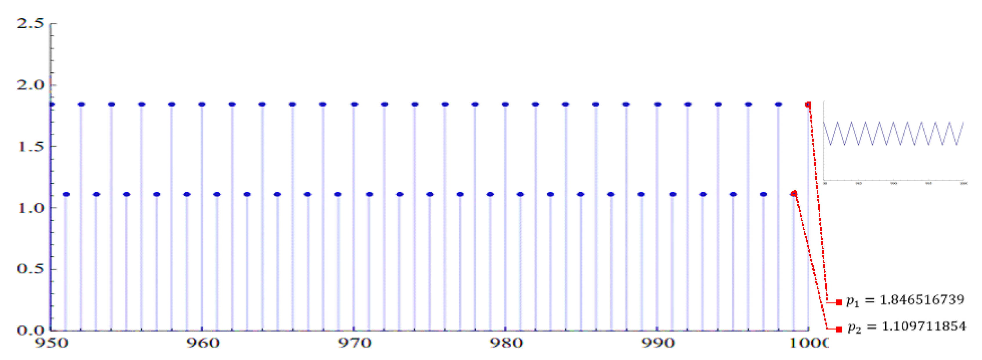
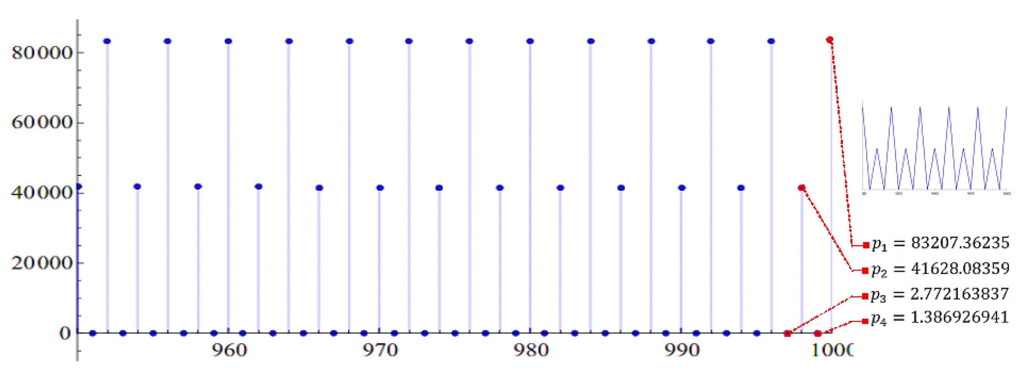
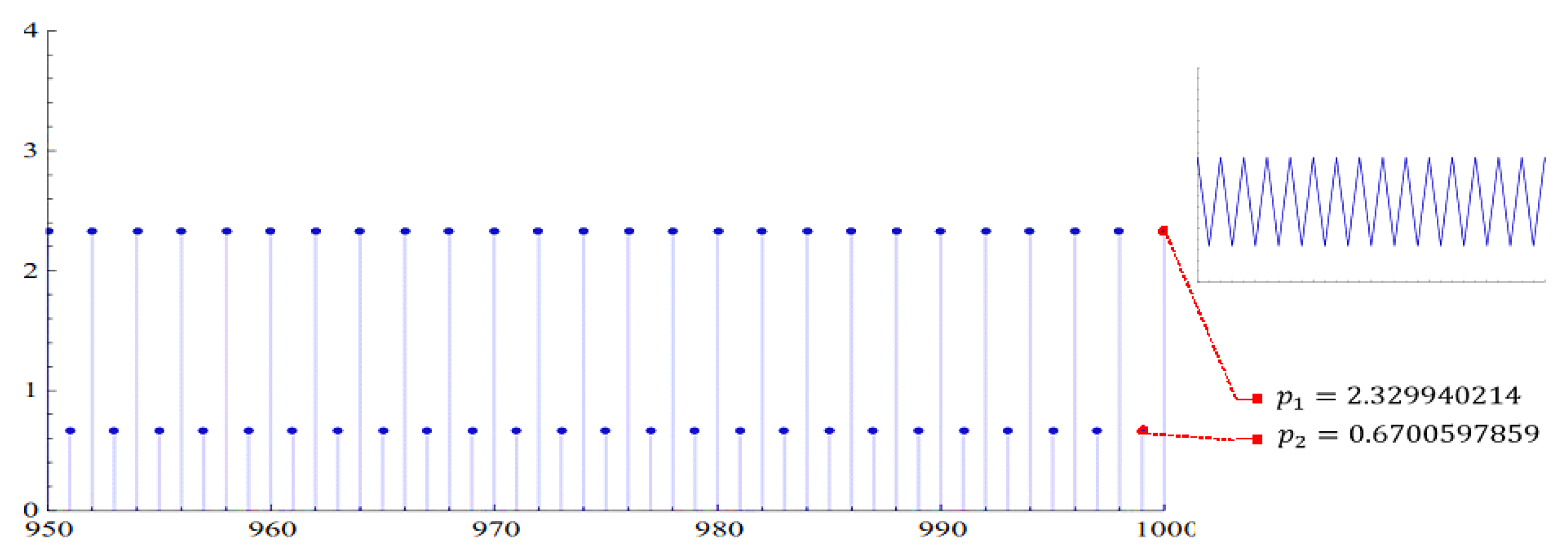
2.2. The Existence of Periodic Solutions

Here, we investigate the periodicity character of the solution for Equation (4).

Lemma 1.

Assume that ${\left\{J_n\right\}}_{n=-1}^{\infty }$ is a solution of Equation (4). Then,

$$J_{m+2k}=a^k{J}_{m}exp\left(-\sum _{i=0}^{k-1}f\left(J_{m+2i+1},J_{m+2i}\right)\right).$$

(24)

Proof. 

Let ${\left\{J_n\right\}}_{n=-1}^{\infty }$ is a solution of Equation (4). From Equation (4), we have

$$\begin{array}{ccc}\hfill J_{m+2k}& =& a{J}_{m+2k-2}exp\left(-f\left(J_{m+2k-1},J_{m+2k-2}\right)\right)\hfill \\ & =& a^2{J}_{m+2k-4}exp\left(-f\left(J_{m+2k-3},J_{m+2k-4}\right)-f\left(J_{m+2k-1},J_{m+2k-2}\right)\right)\hfill \end{array}$$

and so on, we find

$$J_{m+2k}=a^k{J}_{m}exp\left(-\sum _{i=0}^{k-1}f\left(J_{m+2i+1},J_{m+2i}\right)\right).$$

The proof of the lemma is complete. □

Theorem 7.

Assume that $a>1$, ${\left\{J_n\right\}}_{n=-1}^{\infty }$ is a solution of Equation (4) and there exists a couple of integers $\eta \ge -1$ and $k>0$ such that

$$\left({\delta }_{1,k}\right)\sum _{i=0}^{k-2}f\left(J_{ϵ+\eta +2i+1},J_{ϵ+\eta +2i}\right)+D=kln\left(a\right),forϵ=0,1,$$

(25)

where

$$D=f\left(J_{\eta +\left(1-ϵ\right)\left(2k-1\right)},J_{\eta +2k-2+ϵ}\right)and{\delta }_{1,k}=\left\{\begin{array}{cc}1& k\ne 1\\ 0& k=1\end{array}\right..$$

Then ${\left\{J_n\right\}}_{n=-1}^{\infty }$ is an eventually periodic solution with period $2k$.

Proof. 

Assume that there exists an integer number $\eta \ge -1$ such that (25) holds. First, from (25), we have

$$\sum _{i=0}^{k-1}f\left(J_{\eta +2i+1},J_{\eta +2i}\right)=kln\left(a\right)$$

(26)

and

$$\sum _{i=0}^{k-2}f\left(J_{\eta +2i+2},J_{\eta +2i+1}\right)+f\left(J_{\eta },J_{\eta +2k-1}\right)=kln\left(a\right).$$

(27)

Now, from Lemma 1, we get

$$\begin{array}{ccc}\hfill J_{\eta +2k}& =& a^k{J}_{\eta }exp\left(-\sum _{i=0}^{k-1}f\left(J_{\eta +2i+1},J_{\eta +2i}\right)\right)\hfill \\ & =& J_{\eta }exp\left(kln\left(a\right)-\sum _{i=0}^{k-1}f\left(J_{\eta +2i+1},J_{\eta +2i}\right)\right).\hfill \end{array}$$

Using (26), we obtain $J_{\eta +2k}=J_{\eta }$. Also, from Lemma 1, we see that

$$J_{\eta +2k+1}=a^k{J}_{\eta +1}exp\left(-\sum _{i=0}^{k-2}f\left(J_{\eta +2i+2},J_{\eta +2i+1}\right)-f\left(J_{\eta +2k},J_{\eta +2k-1}\right)\right).$$

Since $J_{\eta +2k}=J_{\eta }$ and from (27), we get

$$\begin{array}{ccc}\hfill J_{\eta +2k+1}& =& J_{\eta +1}exp\left(kln\left(a\right)-\sum _{i=0}^{k-2}f\left(J_{\eta +2i+2},J_{\eta +2i+1}\right)-f\left(J_{\eta },J_{\eta +2k-1}\right)\right)\hfill \\ & =& J_{\eta +1}.\hfill \end{array}$$

Similarly, we can prove that

$$J_{\eta +2\nu k+s}=J_{\mu +s}\mathrm{for}\mathrm{all}s=0,1,\dots ,\left(2k-1\right)\mathrm{and}\nu =1,2,\dots .$$

Thus, the sequence ${\left\{J_n\right\}}_{n=-1}^{\infty }$ converges to a prime period $2k$ solutions. The proof of the theorem is complete. □

Corollary 1.

Assume that ${\left\{J_n\right\}}_{n=-1}^{\infty }$ is a solution of Equation (4). If

$$f\left(J_0,J_{-1}\right)=f\left(J_{-1},J_0\right)=lna,$$

then ${\left\{J_n\right\}}_{n=-1}^{\infty }$ is an eventually periodic solution with period $2k$.

In the next theorem, we state a new necessary and sufficient condition for periodic solutions of a period two.

Theorem 8.

Equation (4) has a period two solution $\left\{\dots ,t\sigma ,\sigma ,t\sigma ,\sigma ,\dots \right\}$ if and only if

$$f\left(t,1\right)=f\left(1,t\right)=\frac{1}{\sigma }ln\left(a\right).$$

(28)

Proof. 

Let Equation (4) has a solution of period two $\dots ,\rho ,\sigma ,\rho ,\sigma ,\dots$. Hence, we have

$$\begin{array}{ccc}\hfill \rho & =& \mathsf{\Phi }\left(\sigma ,\rho \right)=a\rho {\mathbf{e}}^{-f\left(\sigma ,\rho \right)}\hfill \\ \hfill \sigma & =& \mathsf{\Phi }\left(\rho ,\sigma \right)=a\sigma {\mathbf{e}}^{-f\left(\rho ,\sigma \right)}.\hfill \end{array}$$

Then, we obtain $f\left(\rho ,\sigma \right)=f\left(\sigma ,\rho \right)$ and hence (28) holds, where $t=\rho /\sigma$. Next, if (28) holds, then we choose $J_{-1}=tln\left(a\right)/f\left(t,1\right),$$J_0=ln\left(a\right)/f\left(1,t\right),t\in \left(0,\infty \right)$ and $t\ne 1$. Thus,

$$\begin{array}{ccc}\hfill f\left(J_0,J_{-1}\right)& =& f\left(\frac{ln\left(a\right)}{f\left(1,t\right)},\frac{tln\left(a\right)}{f\left(t,1\right)}\right)=f\left(\frac{ln\left(a\right)}{f\left(1,t\right)},\frac{tln\left(a\right)}{f\left(1,t\right)}\right)\hfill \\ & =& \frac{ln\left(a\right)}{f\left(1,t\right)}f\left(1,t\right)=ln\left(a\right).\hfill \end{array}$$

Similarly, we can prove that $f\left(J_{-1},J_0\right)=ln\left(a\right)$. Hence, by Corollary 1, it is clear that ${\left\{J_n\right\}}_{n=-1}^{\infty }$ converges to a prime period two solution. The proof of the theorem is complete. □

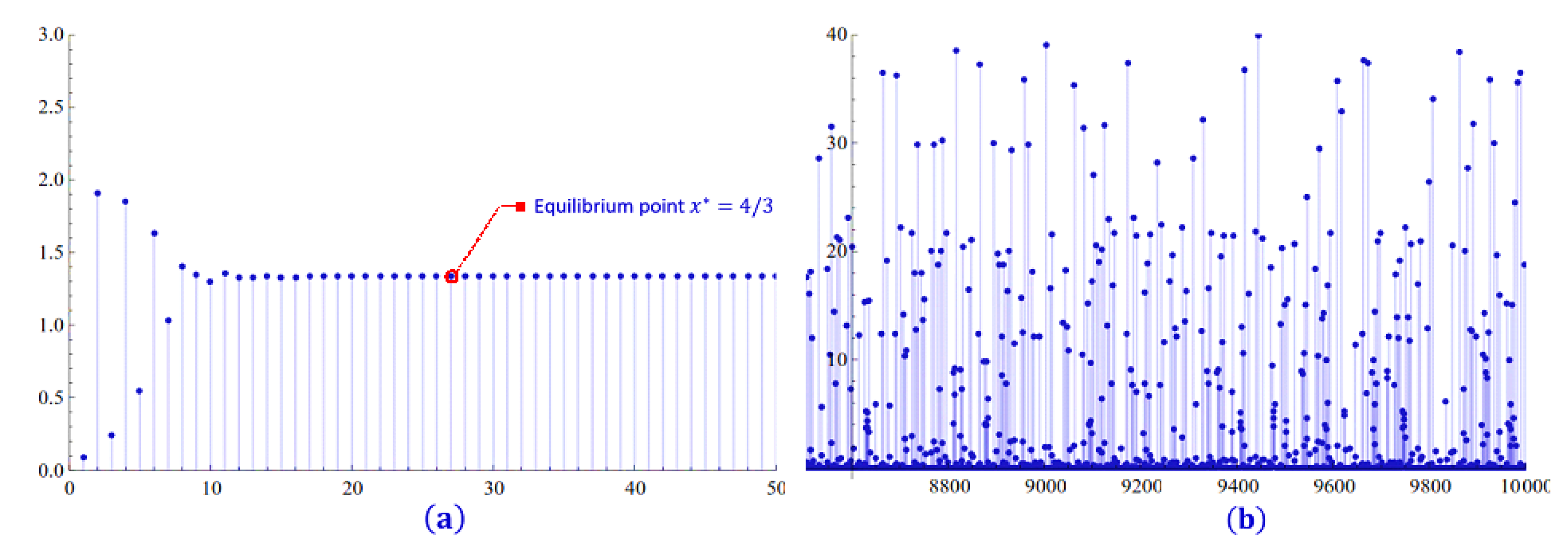
3. A Population Model

Difference equations have been widely used as mathematical models for describing real life situations in biology. In this section, we study the discrete model with two age classes, adults and juveniles (2) where $r,\kappa \in \left(0,\infty \right)$. Expression $exp\left(r-\left(I_n+\alpha J_n\right)\right)$ represents reproduction rate and is a decreasing exponential which captures the over crowding phenomenon as the population grows. To apply our results, we set system (2) as the following

$$J_{n+1}=J_{n-1}{\mathbf{e}}^{r-\left(\kappa J_n+J_{n-1}\right)}.$$

(29)

By compared with (4), we note that $a={\mathbf{e}}^r$ and $f\left(u,v\right)=\kappa u+v$. Thus, we have that $\gamma =f\left(1,1\right)=\kappa +1,\alpha =f_u\left(1,1\right)=\kappa$. Equilibrium points of Equation (29) are $J^{*}=0$ and positive equilibrium $J^{*}=r/\left(\kappa +1\right)$. From Theorem 2, $J^{*}=0$ is an unstable and repeller where $a={\mathbf{e}}^r>1$ for $r>0$.

For locally asymptotically stable of equilibrium point $J^{*}=r/\left(\kappa +1\right)$ of Equation (29), we have the next theorem.

Corollary 2.

We have the following cases:

 1. 

Equilibrium point $J^{*}$ is locally asymptotically stable and sink if and only if $\kappa <1<\frac{2}{r}\left(\kappa +1\right)$.

 2. 

Equilibrium point $J^{*}$ is unstable saddle point if and only if $\kappa >1$.

 3. 

Equilibrium point $J^{*}$ is unstable and repeller if and only if $\kappa <1$ and $r>2\left(\kappa +1\right)$.

 4. 

Equilibrium point $J^{*}$ is nonhyperbolic point if and only if $\kappa =1$, or $\kappa <1$ and $r=2\left(\kappa +1\right)$.

Proof. 

The proof is immediate (from Theorem 3) and hence is omitted. □

Corollary 3.

Every solution of Equation (2) is bounded and $0<J_n\le {\mathbf{e}}^{r-1},$ for all $n>0$.

Proof. 

Since $f\left(u,v\right)=\kappa u+v\ge v$ for all $u\in \left[0,\infty \right)$, we have that, from Theorem 5, every solution of Equation (2) is bounded and $0<J_n\le a/\mathbf{e}={\mathbf{e}}^{r-1}$, and hence the proof is complete. □

Now, we give the periodicity character of the solution for Equation (29).

Corollary 4.

Assume that ${\left\{J_n\right\}}_{n=-1}^{\infty }$ is a solution of Equation (29) and $\kappa =1$. If there exists a positive integer number η such that

$$\sum _{i=0}^{2k-1}{J}_{\eta +i}=kr,$$

(30)

then ${\left\{J_n\right\}}_{n=-1}^{\infty }$ converges to a prime period $2k$ solution.

Remark 1.

Note that, from Corollary 4, if $J_{-1}+J_0=r$, then the solution ${\left\{J_n\right\}}_{n=-1}^{\infty }$ of Equation (4) is a period-two solution.

Theorem 9.

If the solution ${\left\{J_n\right\}}_{n=-1}^{\infty }$ of Equation (29) when $\kappa =1,$ converges to a period-two $\left\{\dots ,\lambda ,r-\lambda ,\lambda ,r-\lambda ,\dots \right\}$ then

$$J_0=\frac{r-\lambda }{\lambda }{J}_{-1}{e}^{\lambda -J_{-1}},$$

(31)

where $\lambda \in \left(0,r\right)$.

Proof. 

From (29), we have

$$\begin{array}{ccc}\hfill J_{n+1}& =& J_{n-1}exp\left(r-\left(J_n+J_{n-1}\right)\right)\hfill \\ & =& J_{n-3}exp\left(2r-\left(J_n+J_{n-1}+J_{n-2}+J_{n-3}\right)\right)\hfill \end{array}$$

and so on, we obtain that

$$\begin{array}{ccc}\hfill J_{n+1}& =& J_{n-2\beta +1}exp\left(\beta r-\left(J_n+J_{n-1}+\dots +J_{n-2\beta +1}\right)\right)\hfill \\ & =& J_{n-2\beta +1}exp\left(\beta r-\sum _{i=0}^{2\beta -1}{J}_{n-i}\right),\beta =0,1,\dots ,\left[\frac{n}{2}\right]+1.\hfill \end{array}$$

(32)

Assume that (4) has a period two solution $\dots ,p,q,p,q,\dots$ [from Corollary 4, we have $\left(p+q\right)=r$]. If $J_{-1}+J_0=r$, then by choosing $\lambda =J_{-1}$, we get that (7) holds. Now, we assume that $J_{-1}+J_0\ne r,$$J_{\eta }\ne q,$$J_{\eta +1}=p$ and $J_{\eta +2}=q$ ($\eta$ even). From (32), we have

$$J_{\eta +1}=J_{\eta -2\beta +1}exp\left(\beta r-\sum _{i=0}^{2\beta -1}{J}_{\eta -i}\right).$$

If we put $\beta =\frac{\eta }{2}+1$, we find

$$J_{\eta +1}=J_{-1}exp\left(\left(\frac{\eta }{2}+1\right)r-\sum _{i=-1}^{\eta }{J}_i\right).$$

(33)

Also,

$$J_{\eta +2}=J_{0}exp\left(\left(\frac{\eta }{2}+1\right)r-\sum _{i=0}^{\eta +1}{J}_i\right).$$

(34)

Combining (33) and (34), we obtain

$$\sum _{i=-1}^{\eta }{J}_i=\left(\frac{\eta }{2}+1\right)r-ln\left(\frac{p}{J_{-1}}\right)$$

(35)

and

$$\sum _{i=0}^{\eta +1}{J}_i=\left(\frac{\eta }{2}+1\right)r-ln\left(\frac{q}{J_0}\right).$$

(36)

Therefore, by (35) and (36), we get

$$\sum _{i=0}^{\eta +1}{J}_i-\sum _{i=-1}^{\eta }{J}_i=ln\left(\frac{p}{J_{-1}}\right)-ln\left(\frac{q}{J_0}\right)$$

and so,

$$J_{\eta +1}-J_{-1}=ln\left(\frac{p{J}_0}{q{J}_{-1}}\right).$$

Hence,

$$J_0=\frac{r-p}{p}{J}_{-1}{e}^{p-J_{-1}}.$$

The proof of the theorem is complete. □

4. Numerical Examples

In order to support our results, we are to consider some numerical examples which illustrate many types of solutions to the Equation (4) and the behavior of these solutions.

Example 1.

Consider the equation

$$J_{n+1}=a{J}_{n-1}exp\left(\frac{J_n{J}_{n-1}}{J_n+J_{n-1}}\right),$$

(37)

where $a>0$. From Theorem 3, the positive equilibrium point $J^{*}=2lna,a>1$, is a nonhyperbolic point. Also, Equation (37) has a prime period 2 solution when $a=2,J_{-1}=5$ and $J_0=3,$ see Figure 1, and prime period 4 solution when $a=8,J_{-1}=20$ and $J_0=30$, see Figure 2.

Example 2.

Consider the Equation (29), if $r=2$ and $k=0.5$, then equilibrium point $J^{*}=4/3$ is a locally asymptotically stable, see Figure 3a. On the other hand, if $r=9$ and $k=1$, then equilibrium point $J^{*}=4/3$ is an unstable saddle point, see Figure 3b.

Example 3.

From Theorem 4, Equation (29) has a prime period $2k$ solution. For example,

 (a) 

If $r=3,\kappa =1,J_{-1}=1$ and $J_0=2.5,$ then Equation (29) has a prime period 2 solution, see Figure 4. Note that,

-

$p=0.6700597859,$$q=2.329940214$ and $p+q=3=r,$ (according to Corollary 4).

-

$J_0=2.5=\frac{r-p}{p}{J}_{-1}{e}^{p-J_{-1}},$ (according to (31) in Theorem 9).

 (b) 

If $r=5,\kappa =1,J_{-1}=2$ and $J_0=2.5$, then Equation (29) has a prime period 6 solution. Note that, $p_1=0.1481492419,$ $p_2=2.052733018,$ $p_3=2.434113484,$ $p_4=3.429195147,$ $p_5=1.026622191,$ $p_6=5.909186918$ and ${\sum }_{i=1}^6{p}_i=15=3r.$

 (c) 

If $r=5,\kappa =1,J_{-1}=2.5$ and $J_0=2.2$, then Equation (29) has a prime period 8 solution.

 (d) 

If $r=5,\kappa =1,J_{-1}=19.6e^{-3.9}$ and $J_0=4.9$, then Equation (29) has a prime period 12 solution.

5. Conclusions

Difference equations have been widely used as mathematical models for describing real life situations in biology. So, this paper is concerned with the qualitative behavior of the solution of the general class of the nonlinear difference equations which involves a population model with two age classes, as a special case. For general equation, we studied the stability (local and global), boundedness and periodicity character (with period $2k$) of the solution. Moreover, by applying our general results on a population model with two age classes, adults and juveniles $J_{n+1}=J_{n-1}{\mathbf{e}}^{r-\left(\kappa J_n+J_{n-1}\right)}$, where expression $exp\left(r-\left(I_n+\alpha J_n\right)\right)$ represents reproduction rate and is a decreasing exponential which captures the over crowding phenomenon as the population grows, we give a complete picture applying the local stability of equilibrium point of population model and we study the boundedness of soluations. Furthermore, we studied the existence of periodic solutions of a prime period-even of this model, as improved and complemented of results of Franke 1999 and conjecture of Kulenovic 2001. In order to support our results, we introduced some numerical examples. Further, we can try to get a necessary and sufficient condition for global stability as well as bifurcation behavior for (4) in the future work.

References

1. Ahmad, S. On the nonautonomous Volterra-Lotka competition equations. Proc. Am. Math. Soc. 1993, 117, 199–204. [Google Scholar] [CrossRef]
2. Allman, E.S.; Rhodes, J.A. Mathematical Models in Biology: An Introduction; Cambridge University Press: Cambridge, UK, 2003. [Google Scholar]
3. Din, Q.; Elsayed, E.M. Stability analysis of a discrete ecological model. Comput. Ecol. Softw. 2014, 4, 89–103. [Google Scholar]
4. Elettreby, M.F.; El-Metwally, H. On a system of difference equations of an economic model. Discr. Dyn. Nat. Soc. 2013, 6, 405628. [Google Scholar] [CrossRef] [Green Version]
5. Haghighi, A.M.; Mishev, D.P. Difference and Differential Equations with Applications in Queueing Theory; John Wiley & Sons Inc.: Hoboken, NJ, USA, 2013. [Google Scholar]
6. Kelley, W.G.; Peterson, A.C. Difference Equations: An Introduction with Applications, 2nd ed.; Harcour Academic: New York, NY, USA, 2001. [Google Scholar]
7. Liu, X. A note on the existence of periodic solutions in discrete predator-prey models. Appl. Math. Model. 2010, 34, 2477–2483. [Google Scholar] [CrossRef]
8. Zhou, Z.; Zou, X. Stable periodic solutions in a discrete periodic logistic equation. Appl. Math. Lett. 2003, 16, 165–171. [Google Scholar] [CrossRef] [Green Version]
9. Cull, P.; Flahive, M.; Robson, R. Difference equations: From rabbits to chaos. In Undergraduate Texts in Mathematics; Springer: New York, NY, USA, 2005. [Google Scholar]
10. Beverton, R.J.H.; Holt, S.J. On the Dynamics of Exploited Fish Populations; Fishery Investigations Series II; Blackburn Press: Caldwell, NJ, USA, 2004; Volume 19. [Google Scholar]
11. May, R.M. Nonlinear problems in ecology and resource management. In Chaotic Behaviour of Deterministic Systems; Helleman, R.H.G., Iooss, G., Stora, R., Eds.; North-Holland Publ. Co.: Amsterdam, The Netherlands, 1983. [Google Scholar]
12. Kocic, V.L.; Ladas, G. Global Behavior of Nonlinear Difference Equations of Higher Order with Applications; Kluwer Academic Publishers: Dordrecht, The Netherlands, 1993. [Google Scholar]
13. Franke, J.E.; Hoag, J.T.; Ladas, G. Global attractivity and convergence to a two-cycle in a difference equation. J. Differ. Equ. Appl. 1999, 5, 203–209. [Google Scholar] [CrossRef]
14. Kulenovic, M.R.S.; Ladas, G. Dynamics of Second Order Rational Difference Equations with Open Problems and Conjectures; Chapman & Hall/CRC Press: Boca Raton, FL, USA, 2001. [Google Scholar]
15. Abu-Saris, R.M.; Devault, R. Global stability of yn+1 = A+yn/yn−k. Appl. Math. Lett. 2003, 16, 173–178. [Google Scholar] [CrossRef] [Green Version]
16. Ahlbrandt, C.D.; Peterson, A.C. Discrete Hamiltonian Systems: Difference Equations, Continued Fractions, and Riccati Equations; Kluwer Academic Publishers: Dordrecht, The Netherlands, 1996; Volume 16. [Google Scholar]
17. Amleh, A.; Grove, E.A.; Georgiou, D.A.; Ladas, G. On the recursive sequence Jn+1 = α+Jn−1/Jn. J. Math. Anal. Appl. 1999, 233, 790–798. [Google Scholar] [CrossRef] [Green Version]
18. Berenhaut, K.S.; Foley, J.D.; Stevic, S. The global attractivity of the rational difference equation yn+1 = 1+yn−k/yn-m. Proc. Am. Math. Soc. 2007, 135, 1133–1140. [Google Scholar] [CrossRef]
19. Border, K.C. Eulers Theorem for Homogeneous Functions; Caltech Division of the Humanities and Social Sciences: Pasadena, CA, USA, 2017. [Google Scholar]
20. Cooke, K.L.; Calef, D.F.; Level, E.V. Stability or chaos in discrete epidemic models. In Nonlinear Systems and Applications; Lakshmikantham, V., Ed.; Academic Press: New York, NY, USA, 1977; pp. 73–93. [Google Scholar]
21. Devault, R.; Kent, C.; Kosmala, W. On the recursive sequence Jn+1 = p+Jn−kJn. J. Differ. Equ. Appl. 2003, 9, 721–730. [Google Scholar] [CrossRef]
22. Devault, R.; Schultz, S.W. On the dynamics of Jn+1 = (βJn+γJn−1)/(BJn+DJn−1). Commun. Appl. Nonlinear Anal. 2005, 12, 35–40. [Google Scholar]
23. Din, Q. A novel chaos control strategy for discrete-time Brusselator models. J. Math. Chem. 2018, 56, 3045–3075. [Google Scholar] [CrossRef]
24. Din, Q. Bifurcation analysis and chaos control in discrete-time glycolysis models. J. Math. Chem. 2018, 56, 904–931. [Google Scholar] [CrossRef]
25. Din, Q.; Elsadany, A.A.; Ibrahim, S. Bifurcation analysis and chaos control in a second-order rational difference equation. Int. J. Nonlinear Sci. Numer. Simul. 2018, 19, 53–68. [Google Scholar] [CrossRef]
26. Elabbasy, E.M.; El-Metwally, H.; Elsayed, E.M. On the difference Equation Jn+1 = (αJn−l+βJnk)/(AJn−l+BJnk). Acta Math. Vietnam. 2008, 33, 85–94. [Google Scholar]
27. El-Owaidy, H.M.; Ahmed, A.M.; Mousa, M.S. On asymptotic behaviour of the differens Equation Jn+1 = α+Jn−1δ/Jnδ. J. Appl. Math. Comput. 2003, 12, 31–37. [Google Scholar] [CrossRef]
28. Elsayed, E.M. Dynamics and behavior of a higher order rational difference equation. Nonlinear Sci. Appl. 2015, 9, 1463–1474. [Google Scholar] [CrossRef] [Green Version]
29. Elsayed, E.M. New method to obtain periodic solutions of period two and three of a rational difference equation. Nonlinear Dyn. 2015, 79, 241–250. [Google Scholar] [CrossRef]
30. Hamza, A.E. On the recursive sequence Jn+1 = α+Jn−1Jn. J. Math. Anal. Appl. 2006, 322, 668–674. [Google Scholar] [CrossRef] [Green Version]
31. Kalabusic, S.; Kulenovic, M.R.S. On the recursive sequnence Jn+1 = (γJn−1+δJn−2)/(CJn−1+DJn−2). J. Differ. Equ. Appl. 2003, 9, 701–720. [Google Scholar]
32. Khuong, V.V. On the positive nonoscillatory solution of the difference equations Jn+1=α+(Jnk/Jnm)p. Appl. Math. J. Chin. Univ. 2008, 24, 45–48. [Google Scholar]
33. Kuang, Y.K.; Cushing, J.M. Global stability in a nonlinear difference-delay Equation model of flour beetle population growth. J. Differ. Equ. Appl. 1996, 2, 31–37. [Google Scholar] [CrossRef]
34. Kulenovic, M.R.S.; Ladas, G.; Sizer, W.S. On the dynamics of Jn+1=(αJn+βJn−1)/(γJn+δJn−1). Math. Sci. Res. Hot-Line 1998, 2, 1–16. [Google Scholar]
35. Moaaz, O.; Chalishajar, C.; Bazighifan, O. Some qualitative behavior of solutions of general class difference equations. Mathematics 2019, 7, 585. [Google Scholar] [CrossRef] [Green Version]
36. Moaaz, O. Comment on new method to obtain periodic solutions of period two and three of a rational difference Equation [Nonlinear Dyn 79:241250]. Nonlinear Dyn. 2017, 88, 1043–1049. [Google Scholar] [CrossRef]
37. Pielou, E.C. An Introduction to Mathematical Ecology; John Wiley & Sons: New York, NY, USA, 1965. [Google Scholar]
Figure 1. Prime period 2 solution.
Mathematics 08 00516 g001
Figure 2. Prime period 4 solution.
Mathematics 08 00516 g002
Figure 3. (a) Locally asymptotically stable, (b) unstable saddle point.
Mathematics 08 00516 g003
Figure 4. Prime period 2 solution.
Mathematics 08 00516 g004