Clusters in Separated Tubes of Tilted Dipoles

Abstract

A few-body cluster is a building block of a many-body system in a gas phase provided the temperature at most is of the order of the binding energy of this cluster. Here we illustrate this statement by considering a system of tubes filled with dipolar distinguishable particles. We calculate the partition function, which determines the probability to find a few-body cluster at a given temperature. The input for our calculations—the energies of few-body clusters—is estimated using the harmonic approximation. We first describe and demonstrate the validity of our numerical procedure. Then we discuss the results featuring melting of the zero-temperature many-body state into a gas of free particles and few-body clusters. For temperature higher than its binding energy threshold, the dimers overwhelmingly dominate the ensemble, where the remaining probability is in free particles. At very high temperatures free (harmonic oscillator trap-bound) particle dominance is eventually reached. This structure evolution appears both for one and two particles in each layer providing crucial information about the behavior of ultracold dipolar gases. The investigation addresses the transition region between few- and many-body physics as a function of temperature using a system of ten dipoles in five tubes.

1. Introduction

One important question that quantum few-body physics should answer is under which conditions few-body bound states play a role (or could be observed) in a many-body system. It is clear that if the energy associated with the temperature is much larger than the few-body binding energy, then bound states occupy a tiny fraction of the Hilbert space, and hence the probability to observe (populate) a bound state is exponentially suppressed. Think, for example, about Efimov states [1] (see References [2,3,4,5] for a review) in cold-atom systems. These states are always present in a cold gas; however, only at ultracold temperatures is it possible to observe them [6].

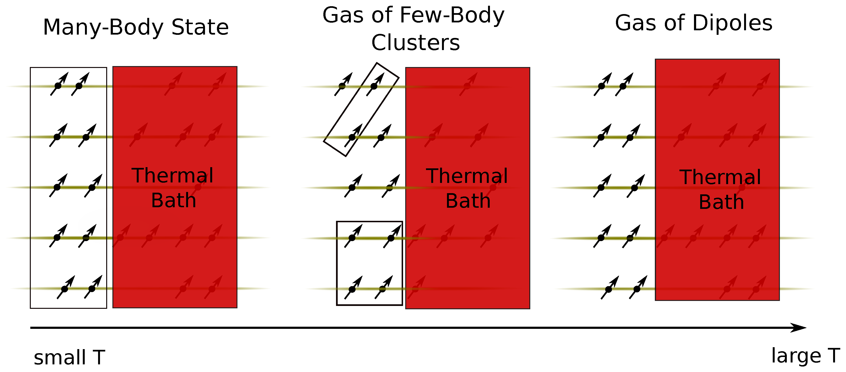
In this paper, we study at which temperatures few-body bound states can be observed in a cold gas of dipoles (see [7,8], which review cold dipolar gases), once precise control of cold polar molecules is achieved [9]. Our model is the system illustrated in Figure 1. The dipoles are trapped by an optical lattice, which can be formed, for example, by superimposing two orthogonal standing waves [10]. Strong trapping prevents particles from tunneling between the tubes, so the system can be approximated as a collection of one-dimensional tubes. An external electric field controls the alignment of the dipoles. Previous works investigated the formation of chains in two-dimensional geometries [11]. We are interested in formation of few-body states with more than one particle per layer (or tube), which are unlikely to be observed for dipoles with perpendicular polarization [12]. Therefore, we assume that the dipoles are tilted to the “magic angle” such that there is no interaction within a tube, see, References [12,13] for a discussion of few-body bound states with other polarizations. Still the long-range dipole-dipole interaction allows particles to interact between the layers. This interaction supports a zoo of few-body bound states [12,13,14,15], whose presence should be taken into account when building models of the corresponding many-body systems (see, for example, [11,16,17,18,19]).

To find at which temperature these states enter the description, we consider a system of dipoles coupled to a thermal bath. We assume that particles obey Boltzmann statistics, however, we will argue that our results are also applicable to systems of bosons. For the sake of discussion, we assume that the system is made of ten dipoles that occupy five tubes, see Figure 1. In spite of its simplicity, we expect that this system contains all basic ingredients allowing us to learn about the formation of the simplest few-body clusters. This system has enough tubes so that particles in the outermost tubes do not interact with each other. Therefore, adding more tubes cannot qualitatively change our results. Moreover, the system has more than one particle per tube allowing us to investigate the effect of non-chain few-body structures. Our results show that these structures are not important for our analysis. In particular, our results show that there is a clear transition from a many-body bound state to a state dominated by chains of dipoles.

This paper is organized as follows. In Section 2, we introduce the method used for computation of few-body energies. The partition function that determines the probability of a particular state is discussed in Section 3. In Section 4, we demonstrate at which temperatures few-body clusters can be observed. In Section 5, we summarize our results and conclude.

2. Binding Energies of Clusters

The binding energy of a specific cluster can be obtained by diagonalizing the Hamiltonian

$$\begin{array}{ccc}\hfill H^{dd}& =& -\frac{{ħ}^2}{2m}\sum _{i,\alpha }\frac{d^2}{d{x}_{i,\alpha }^2}+\sum _{i,j;\alpha >\beta }{V}_{dip}(x_{i,\alpha }-x_{j,\beta }),\hfill \end{array}$$

(1)

where m is the mass of the dipolar particle, the subscript $\{i,\alpha \}$ refers to the ith particle in the $\alpha$th layer. The potential, $V_{dip}$, describes the dipole-dipole interaction:

$$V_{dip}(x_{i,\alpha }-x_{j,\beta })=\frac{{\mathbf{D}}_{i,\alpha }{\mathbf{D}}_{j,\beta }{r}^2-3\left({\mathbf{D}}_{i,\alpha }\mathbf{r}\right)\left({\mathbf{D}}_{j,\beta }\mathbf{r}\right)}{r^5},$$

(2)

where $\mathbf{r}=(x_{i,\alpha }-x_{j,\beta },0,nd)$ is the relative distance between the two dipoles, $n=\alpha -\beta$ determines the separation between the dipoles in the z direction, d is the distance between the adjacent tubes and ${\mathbf{D}}_{i,\alpha }$ is the dipole moment of the ith dipole in the $\alpha$th layer. For simplicity, the width of a tube is taken to be zero (for finite widths, see References [14,20,21]). By assumption, the dipole moment has only x and z components: ${\mathbf{D}}_{i,\alpha }=D_{i,\alpha }(\cos \left(\varphi \right),0,\sin \left(\varphi \right))$. Our choice for the tilting angle, $\varphi$, will be discussed shortly. Therefore, we write

$$V_{dip}\left(x\right)=U\frac{x^2+{\left(nd\right)}^2-3{\left[x\cos \varphi +nd\sin \varphi \right]}^2}{{\left(x^2+{\left(nd\right)}^2\right)}^{5/2}},$$

(3)

where U determines the strength of the dipole-dipole interaction. Values of U are in units of ${ħ}^{2}d/m$ unless otherwise noted.

It is complicated, if not impossible, to calculate exactly binding energies of $H^{dd}$ for large clusters of dipoles. Instead, we resort to a harmonic approximation. The model of choice, coupled quantum harmonic oscillators,

$$H^{osc}=-\frac{{ħ}^2}{2m}\sum _i\frac{d^2}{d{x}_{i,\alpha }^2}+\frac{\mu }{4}\sum _{i,j,\alpha ,\beta }{\omega }_{\alpha \beta }^2{(x_{i,\alpha }-x_{j,\alpha }-b_{\alpha \beta })}^2+V^{shift},$$

(4)

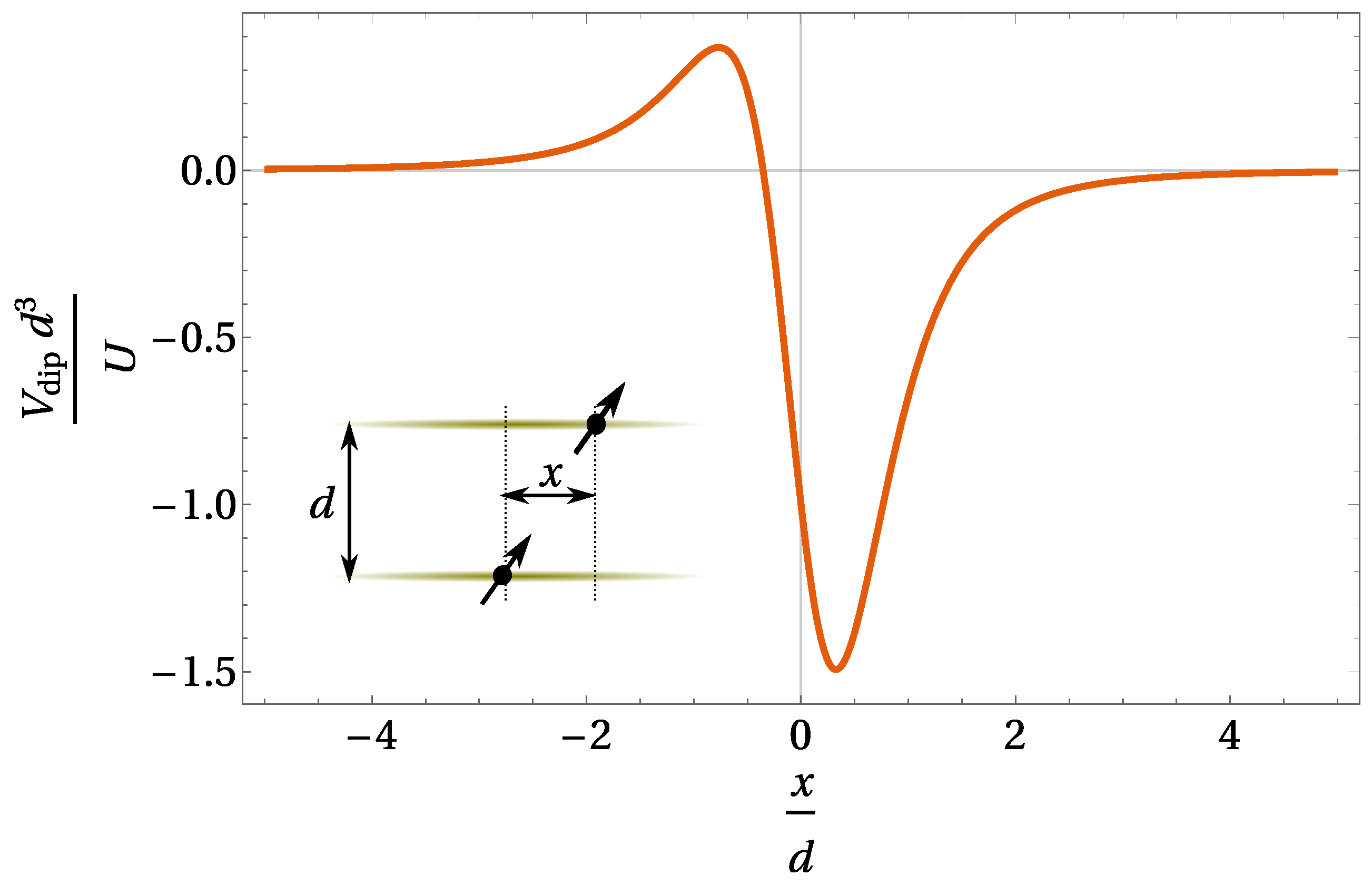
is exactly solvable [22]. Here $\mu =m/2$ is the reduced mass of the dipolar particles, ${\omega }_{\alpha \beta }$ is the coupling frequency between particles in different layers (if $\alpha =\beta$ then ${\omega }_{\alpha \beta }=0$), $b_{\alpha \beta }$ is the origin shift of the coupling frequency, and $V^{shift}$ is a constant energy shift. The parameter $b_{\alpha \beta }$ is present because a spatially shifted oscillator more accurately reflects $V_{dip}$, as the minimum of $V_{dip}$, in general, does not occur at $x=0$ (see Figure 2).

The parameters of Equation (4) should be adapted to the system of interest depicted in Figure 1. Our philosophy is that the properties of two dipoles in adjacent layers should be reproduced by our oscillator model. The dipoles experience an overall attraction for $U>0$ (i.e., $\int V_{dip}\left(x\right)\mathrm{d}x<0$), which leads to a two-body bound state in one spatial dimension at any interaction strength [23,24]. We would then like to use the energy of this two-body state, as well as its size, to determine the parameters of $H^{osc}$: ${\omega }_{\alpha \beta }$, $b_{\alpha \beta }$ and $V^{shift}$. These parameters are obtained by variationally solving the exact Hamiltonian from Equation (1) for two particles:

$$H_2^{dd}=-\frac{{ħ}^2}{2\mu }\frac{d^2}{d{x}^2}+V_{dip}\left(x\right),$$

(5)

where x is the relative in-tube distance between two dipoles.

To establish the coupling frequency between adjacent layers, ${\omega }_{12}$, and $b_{12}$ we find the function of the Gaussian form, $\psi \propto \exp (-A{(x-B)}^2)$, that minimizes the expectation value of $H_2^{dd}$. We note that the function $\psi$ is the ground state of the Hamiltonian from Equation (4) for two particles, i.e.

$$H_2^{osc}=-\frac{{ħ}^2}{2\mu }\frac{d^2}{d{x}^2}+\frac{\mu {\omega }_{12}^2{(x-b_{12})}^2}{2}+V_2^{shift},$$

(6)

whose frequency, ${\omega }_{12}$, is related to the variational parameter A by ${\omega }_{12}=2Aħ/\mu$ and $b_{12}=B$. The energy shift, $V_2^{shift}$, is used in $H_2^{osc}$ to set the two-body energy at the correct position, $V_2^{shift}=E_2-ħ{\omega }_{12}/2$, where $E_2$ is the exact ground state energy of $H_2^{dd}$. We calculate this energy by solving the Schrödinger equation in coordinate space. We first use a lattice grid to discretize the kinetic energy operator, which leads to a linear system of equations. This system is then solved by matrix diagonalization. The error can be made arbitrarily small by increasing the number of points used for discretization. Therefore, all parameters of $H^{osc}$ for two particles are determined. To set the interactions that appear in $H^{osc}$ beyond adjacent layers, we use the scaling properties (see Reference [25]) of the dipole-dipole Hamiltonian (5) to adjust the frequencies and shifts:

$$\begin{array}{c}\hfill {\omega }_{\alpha \beta }=\frac{{\omega }_{12}(U/\alpha -\beta )}{{(\alpha -\beta )}^2},\end{array}$$

(7)

$$\begin{array}{c}\hfill b_{\alpha \beta }=\frac{b_{12}(U/\alpha -\beta )}{{(\alpha -\beta )}^2},\end{array}$$

(8)

$$\begin{array}{c}\hfill V_{2,\alpha \beta }^{shift}=\frac{E_2(U/\alpha -\beta )}{{(\alpha -\beta )}^2}-\frac{ħ{\omega }_{\alpha \beta }}{2},\end{array}$$

(9)

where the functions ${\omega }_{12}\left(U\right)$, $b_{12}\left(U\right)$, and $E_2\left(U\right)$ describe the dependence on the dipole strength of the frequency, origin shift, and two-body energy, respectively. They are obtained by following the variational procedure described above for a set of values of U. The scaling properties are obtained by making the Hamiltonian dimensionless, by using the inter-layer distance, d, as the unit of length, and then seeing how the different quantities scale with this distance. The dimensionless Schrödinger equation is

$$-\frac{1}{2}\frac{d^2\psi }{d{\overline{x}}^2}+\frac{Um}{{ħ}^{2}d}\frac{({\overline{x}}^2-2)}{{({\overline{x}}^2+1)}^{5/2}}\psi =\frac{Em{d}^2}{{ħ}^2}\psi ,$$

(10)

where $\overline{x}=x/d$. From this equation, it can be seen that the dipole strength scales with $1/d$ and that the energy must be scaled by $1/d^2$, affecting the shift as shown in Equation (9). Regarding the other two scaling relationships, the expectation value of a two-body Hamiltonian can be written as

$$E_{exp}=\sqrt{\frac{\pi }{2A}}\int e^{-2A{(x-B)}^2}\left(-\frac{{ħ}^2}{2m}\frac{{\partial }^2}{\partial x^2}+V_{dip}\left(x\right)\right)\mathrm{d}x,$$

(11)

which means that $E_{exp}=\frac{{ħ}^2}{m{d}^2}G({\omega }_{12}{d}^2,b_{12}/d,U/d)$, where G is some function. Equations (7) and (8) follow from the functional form of $E_{exp}$.

For all our calculations, we consider the angle, $\varphi$, to be the so-called “magic angle”, ${\varphi }_m$. This is the angle where the intra-layer interaction, $V_{dip}$, vanishes, and is determined by $\cos \left({\varphi }_m\right)=1/\sqrt{3}$ (${\varphi }_m\approx {54.7}^{\circ }$). The inter-layer interaction is presented in Figure 2. To explain our choice of angle, we discuss below what happens if $\varphi <{\varphi }_m$ or $\varphi >{\varphi }_m$. If $\varphi <{\varphi }_m$, then there is attraction between particles within the layers. We do not consider this case further, because a many-body system of attractive dipoles collapses, i.e., the limit ${lim}_{N\to \infty }{E}_N/N$ is not a finite number (cf. Reference [26] for bosons interacting with zero-range potentials). We note that one could stabilize the system of attractive bosons by including a short-range repulsion, see, e.g., theoretical works References [27,28,29] inspired by recent observations of coherent droplets in dipolar systems [30,31,32,33]. We do not investigate this possibility here. For $\varphi >{\varphi }_m$, there is repulsion within the same tube and attraction between the tubes. We modeled this system with two-dimensional layers before [25] with an inverted oscillator representing the repulsion. While this reasonably modeled how such a system might fall apart, the inverted oscillator was difficult to constrain, and we sought a more realistic way of representing the repulsion. With the results found in [34,35,36,37], showing that we could treat the individual layers separately, we inserted the exact repulsion in the in-layer energies, coupled with harmonic attraction between the layers. This treatment failed to agree with earlier SVM calculations in Reference [12]. For example, it was found that even at 55${}^{\circ }$ (just past the “magic angle”), the oscillator model had energies that were noticeably different from what was calculated before. This happened because the long-range in-layer dipole-dipole repulsion pushes the particles far from each other into the region, where the harmonic oscillator does not reproduce well the intra-layer attraction. Therefore, in the present work, calculations are performed at the “magic angle” only.

Now all parameters of $H^{osc}$ are determined (note that $V^{shift}$ from Equation (4) is the sum of all the $V_2^{shift}$ for all pairs). We can move on to calculating energies of clusters. However, before that, we note that there are other ways to determine the parameters of $H^{osc}$. One could, for example, avoid using $V^{shift}$ and establish frequencies variationally, similar to two-dimensional calculations of Reference [11]. An advantage of such an approach would be that the obtained energies rigorously establish an upper bound on the energy. A disadvantage of neglecting $V^{shift}$ would be that a Gaussian wave function fails to describe weakly bound states. For example, it predicts a critical value for two-body binding in two spatial dimensions [11]. One could also estimate the parameters of $H^{osc}$ from $V_{dip}$ (see Figure 2) using the limit of large U, i.e., when particles move only in the vicinity of the potential minimum. The interaction potential close to its minimum can be written as

$$V_{dip}=-U\frac{d^2+2\sqrt{2}xd}{{(d^2+x^2)}^{5/2}}\simeq \frac{U}{d^3}\left[-1.49+4.34{\left(\frac{x}{d}-x_m\right)}^2-3.32{\left(\frac{x}{d}-x_m\right)}^3-5.03{\left(\frac{x}{d}-x_m\right)}^4\right],$$

(12)

where $x_m=\frac{3\sqrt{17}-5}{16\sqrt{2}}$ determines the position of the minimum of $V_{dip}$. This expansion leads to an estimate of the ground state energy

$$\begin{array}{c}\hfill E_2=-1.49\frac{U}{d^3}+\sqrt{4.34\frac{U}{d^3}\frac{{ħ}^2}{m{d}^2}}-0.869\frac{{ħ}^2}{m{d}^2},\end{array}$$

(13)

the first two terms here are calculated using the first two terms in the expansion in Equation (12), the last term is calculated considering the last terms in Equation (12) as perturbations. According to this estimate, $V_{dip}$ can be approximated by a harmonic oscillator potential if $-1.49\frac{U}{d^3}+\sqrt{4.34\frac{U}{d^3}\frac{{ħ}^2}{m{d}^2}}\gg 0.869\frac{{ħ}^2}{m{d}^2}$, which is not satisfied for parameter regimes we consider below. We leave an exploration of different ways to determine parameters of $H^{osc}$ to future studies. Instead, we compare the energies from our oscillator model to the exact results.

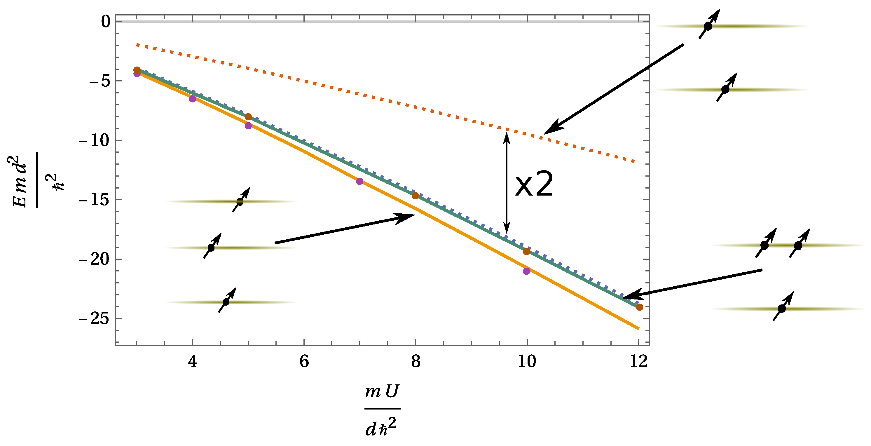
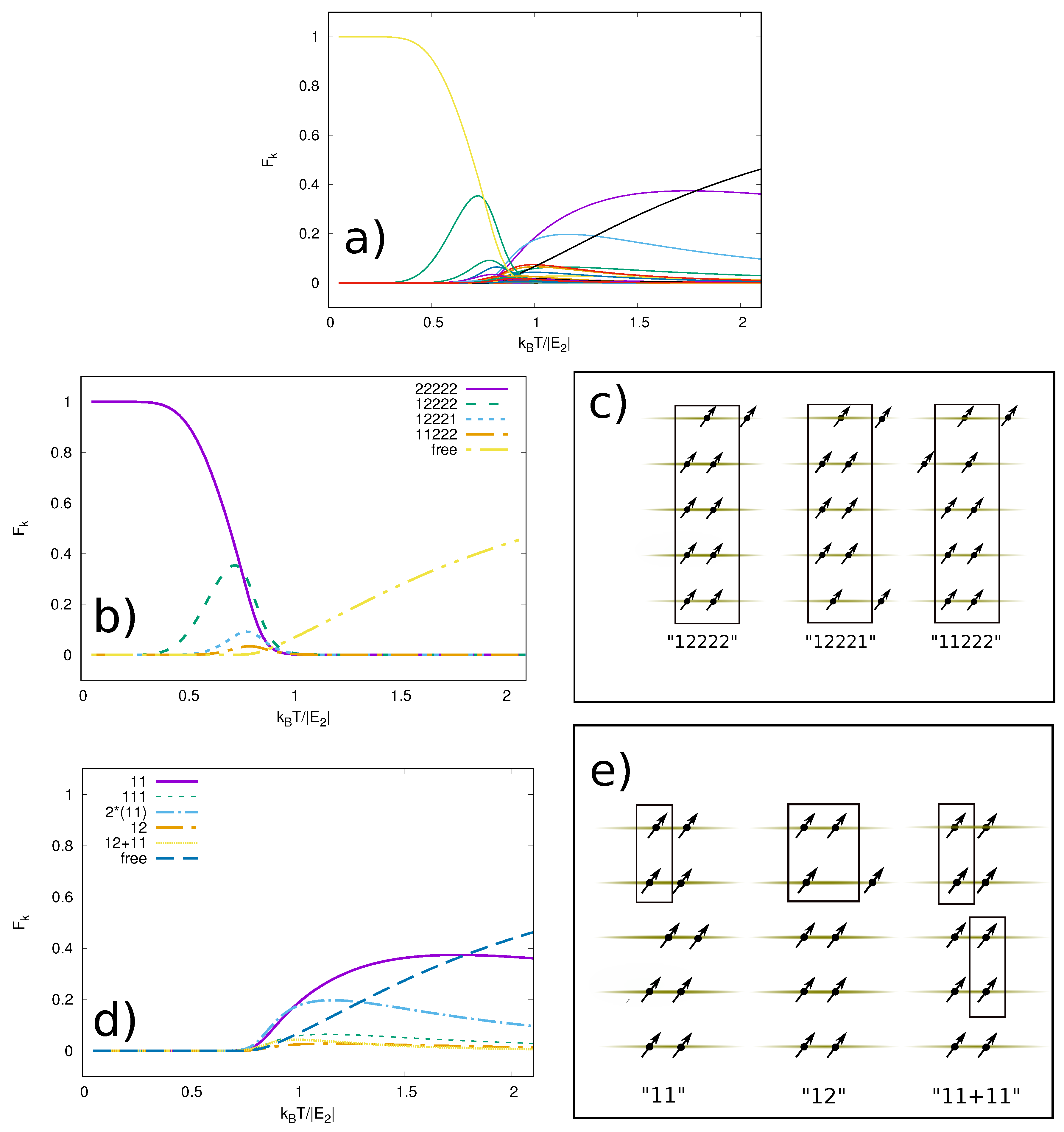
For convenience, we first introduce the labeling for bound states (see Figure 3): 11 means a bound state made of two particles in adjacent layers, 12 refers to two particles in one layer and a single particle in the adjacent layer, 111 is a bound state of three particles with one particle per tube, etc. After determining all parameters of the oscillator model, we compare the ground state energies of free (no external trap) few-body systems obtained in the oscillator model with results calculated with the stochastic variational method (SVM) (for the description of the method see [38,39]).

These comparisons can be seen in Figure 3; we also tabulate energies for certain values of U in

Table 1. Comparison between the harmonic oscillator (HO) model and the stochastic variational method (SVM) in obtaining energies for few-body dipolar clusters. The different clusters are three and four particle chains (labeled 111 and 1111, respectively), and a system with two particles in one layer and a single particle in the adjacent layer (labeled 12). The units of energy are ${ħ}^2/\left(m{d}^2\right)$, and the units of U are ${ħ}^{2}d/m$.

U	111 (HO)	111 (SVM)	1111 (HO)	1111 (SVM)	12 (HO)	12 (SVM)
3	−4.35	−4.45	−6.88	−7.11	−4.02	−4.01
5	−8.67	−8.81	−13.63	−13.95	−8.04	−8.02
10	−20.67	−20.97	−32.33	−32.96	−19.31	−19.30

. The harmonic oscillator and variationally obtained results are indeed very close in all cases. This is also demonstrated in Figure 3, where the results of the two methods are compared. They agree very well, with the worse comparisons within about 1.5%. Similar comparisons for chains of dipoles can be found in Reference [12]. For our further calculations, we will use only the ground state energies of $H^{osc}$. We assume that for a given cluster, the population of all bound excited states is negligible in comparison to the population of the ground state. To validate this assumption, we note that for small values of U there are no excited states. We find numerically that the first excited bound state for two particles in two adjacent layers appears at $U\simeq 3.7{ħ}^{2}d/m$. The excited states remain weakly bound for all considered values of U. For example, for $U=8{ħ}^{2}d/m$, the ground state is about $7.43$ times more bound than the first excited state. Each weakly two-body state gives rise to a family of shallow few-body states. These states have small binding energies, which allows us to refrain from considering them here. Finally, let us give an estimate for the temperature scales that correspond to the calculated binding energies. We assume that $d=0.5\mu$m and $m=m{(}^6{\mathrm{Li}}^{133}\mathrm{Cs})$, which leads to $E_2\simeq 50nK\times k_B$ for $U=5$, where $k_B$ is the Boltzmann constant. Smaller values of U require even smaller temperatures for observation of few-body clusters, therefore, in what follows we focus on $U=5$ and $U=8$.

3. Abundances of Clusters

We consider five layers, each with two dipolar molecules (particles) inside. We assume that every particle is in the harmonic oscillator, $m{\omega }_0^2{x}_{i,\alpha }^2/2$. This can be either due to an external trapping potential, or a way to simulate a finite density of a many-body system. We then calculate the fractional occupancy of given clusters as a function of temperature. For simplicity, we assume that the particles are distinguishable, thus they obey Boltzmann statistics. We discuss this assumption in detail at the end of the next section.

Few-body clusters range from the simplest, a two-particle bound state of particles in adjacent layers, up to a bound state of all ten particles. We also include the possibility that all ten remain unbound, in which case the energies are approximately given by the energies of the states of the confining harmonic trap of the layer. The fractional occupancy of any state k is

$$f_k=\frac{e^{-\beta E_k}}{Z},$$

(14)

where $E_k$ is the energy of state k, Z is the partition function and $\beta =1/k_{B}T$. The partition function in the canonical ensemble is

$$Z=\sum _k{g}_k{e}^{-\beta E_k},$$

(15)

where $g_k$ is the degeneracy of the kth energy. We write the energy of the various cluster configurations as a sum of two components:

$$\begin{array}{ccc}\hfill E_k& =& \sum _{\mathrm{bound}}\left[{ϵ}_j+ħ{\omega }_0\left(n_j^{CM}+\frac{1}{2}\right)\right]+ħ{\omega }_0\sum _{\mathrm{free}}\left(n_l+\frac{1}{2}\right)\hfill \\ & =& {\mathcal{E}}_k+\left({\mathcal{N}}_{\nu }+\frac{\nu }{2}\right)ħ{\omega }_0.\hfill \end{array}.$$

(16)

The first component, ${\mathcal{E}}_k={\sum }_{\mathrm{bound}}{ϵ}_j$, is the binding energy of all clusters in the state k, with ${ϵ}_j$ being the binding energy of the jth cluster in the configuration k. The first line in Equation (16) also contains sums over all the various oscillator degrees of freedom in the configuration. The free particles are particles moving in the oscillator potential defined by ${\omega }_0$, with the corresponding energy levels and quantum numbers, $n_l$. The center of masses (CM) of the cluster(s) also have the same spectrum. To simplify notation, we introduce the quantum number ${\mathcal{N}}_{\nu }\equiv {\sum }_{\mathrm{bound}}{n}_j^{CM}+{\sum }_{\mathrm{free}}{n}_l$. 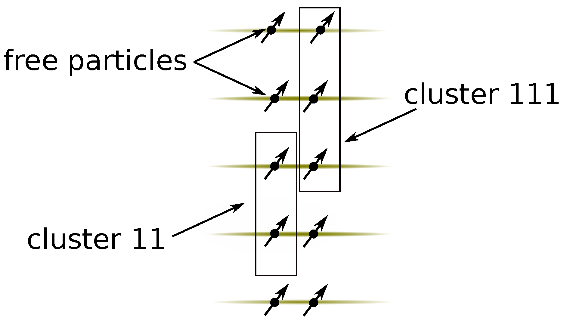The value of $\nu$ defines how many oscillator degrees of freedom we have. To illustrate the decomposition of the energy $E_k$, let us consider the configuration k presented in Figure 4. This configuration has two clusters and five free particles. The energy ${\mathcal{E}}_k$ is the sum ${ϵ}_{11}+{ϵ}_{111}$. The value of ${\mathcal{N}}_{\nu }$ can take any integer value. It is given by the decomposition ${\mathcal{N}}_{\nu =7}={\sum }_{i=1}^7{n}_i$, where $n_i=0,1,2\dots$.

The energy, ${ϵ}_j$, is obtained by using the harmonic approximation from the previous section. By construction, ${ϵ}_j$ is not affected by the harmonic oscillator potential, $m{\omega }_0^2{x}_{i,\alpha }^2/2$, whose length is much larger than the size of the cluster. Please note that to write the energy $E_k$, we assume that the cluster-cluster and cluster-(free particle) interactions are negligible. This assumption relies on the two observations: (i) by construction, the harmonic oscillator length is much larger than the range of the dipole-dipole potential, therefore, for low-lying excited states we may approximate $V_{dip}$ with a zero-range interaction; (ii) the interaction due to a short-range potential can shift the energy by only about $ħ{\omega }_0$. This statement relies on comparing the energies in a weakly interacting limit to that of a strongly interacting limit for zero-range interaction models, see, e.g., References [40,41]. This shift is not important for our qualitative discussion.

For a specific state, the CM and the free motion would also appear with specific quantum numbers. Since we are primarily interested in which specific clusters are prevalent at a given temperature, we then include all possible oscillator excitations by summing them up, so that the probability of a specific cluster configuration, $F_k$, is given by summing $f_k$ from Equation (14)

$$F_k=\frac{g_k}{Z}{e}^{-\beta \left({\mathcal{E}}_k+\frac{{\nu }_kħ{\omega }_0}{2}\right)}{\left(\frac{1}{1-e^{-\beta ħ{\omega }_0}}\right)}^{{\nu }_k},$$

(17)

where ${\mathcal{E}}_k$, ${\nu }_k$, along with the degeneracy $g_k$ must be determined for each cluster configuration. The partition function, extracted from the condition that $\sum f_k=1$, is then

$$Z=\sum _k{g}_k{e}^{-\beta \left({\mathcal{E}}_k+\frac{{\nu }_kħ{\omega }_0}{2}\right)}{\left(\frac{1}{1-e^{-\beta ħ{\omega }_0}}\right)}^{{\nu }_k}.$$

(18)

As an example, consider the cluster configuration in Figure 4. We have $\nu =7$, since there are five free particles, the CM of the 11 cluster, and the CM of the 111 cluster. The binding energy of the clusters is given by ${\mathcal{E}}_k={ϵ}_{11}+{ϵ}_{111}$. There are 176 ways to distribute the clusters 11 and 111 among five different layers. Therefore $g_k=176$, and furthermore, the probability to find a configuration with a single 11 cluster and a single 111 cluster is given by

$$F_{11+111}=\frac{176}{Z}{e}^{-\beta ({ϵ}_{11}+{ϵ}_{111}+\frac{7}{2}ħ{\omega }_0)}{\left(\frac{1}{1-e^{-\beta ħ{\omega }_0}}\right)}^7,$$

(19)

where we introduced the convention that $A+B$ means that the clusters $A(=11)$ and $B(=111)$ exist simultaneously in the system.

4. Results and Discussion

Numerical applications of the formulation quickly contain many configurations. In the present report, we restrict ourselves to two relatively simple systems, yet sufficiently complicated to reveal general features.

4.1. One Particle per Tube

The first system considered is five layers each with one particle. There are seven different clusters in this system: chains of five, four, three, and two particles, five free particles, two separate chains of two particles each, and finally a chain of three particles separate from a chain of two particles. We do not consider clusters consisting of four particles when the middle layer is empty, because our clusters should at least have one particle in a layer linking them together. Otherwise they are very weakly bound and effectively separate structures.

The energy of the system as function of temperature is first calculated as the Boltzmann weighted average over cluster configurations. The results are shown in Figure 5 for different interactions and trap frequencies. The overall behavior of the energies is not surprisingly a move from the ground state values at low temperature to the high-temperature limit of $5k_{B}T$ for five free particles in the present system. This limit is seen by comparing to the temperature dependent average energy of five free particles. This limit is almost reached at a temperature of about the dimer bound-state energy of two particles in adjacent layers.

Results for fractional occupancies are shown in Figure 6a, where we see that the dominant cluster is the fully bound 5-particle chain at low temperature. Its occupancy decreases rather quickly from unity to zero, and as the temperature increases, the less-bound structures appear. The free-particle occupancy increases steadily as expected towards unity at high temperature. The free particles are already dominating at intermediate temperature, where the second largest contribution consists of bound dimer systems.

In Figure 6b, the interaction strength increased to $U=8$ in comparison to Figure 6a, but the plots are very similar, since the x-axis is scaled by the two-body binding energy. In both cases, at just under $k_{B}T/E_2=0.5$, we see the most mixed system with most of the clusters having significant abundance. None have a fraction greater than about 0.2 at this temperature. Please note that the $U=5$ plot appears to show slightly longer tails into higher temperatures.

Figure 6c changes the confinement frequency. This effectively changes the density of the particles in a tube, since the oscillator length of the tube, $b=\sqrt{ħ/m{\omega }_0}$ is changed by changing ${\omega }_0$. For the sake of argument, we relate this length to the distance between the layers, obtaining the relationship ${\omega }_0\propto 1/\left({\alpha }^2{d}^2\right)$, where $\alpha$ is a scaling factor that can be experimentally controlled. In Figure 6c we then take $\alpha =\sqrt{10}$, which decreases the density of the layer, while keeping the interaction strength the same as in Figure 6a. The primary effect is similar to increasing the interaction strength that is shifting the emergence of smaller fragments to smaller temperatures.

This is emphasized in Figure 6d, which has both $U=8$ and decreased density, and the “melting” of the fully bound cluster occurs at the smallest temperature. The relative maxima of the curves remain of a similar height in all the plots. Therefore, interaction strength and confinement frequency can cause similar movements on the temperature scale. It may appear from glancing at Figure 6 that the interaction strength does not have a large effect on our results. Recall, however, that the x-axis has been scaled by the two-body energy, which is greatly influenced by the interaction strength. The figures would be quite different without this scaling. The re-scaling makes it clear that the two-body energy sets the relevant energy scale for the system.

4.2. Two Particles per Tube

When we include two particles per tube, the number of clusters increases dramatically. There are 119 non-degenerate cluster configurations, and we do not consider any clusters where there is an empty tube between different members of the cluster. An intermediate attractive ingredient is again needed to provide an effectively bound system in contrast to separate configurations.

In Figure 7 we show the average energy compared to the energy of ten free particles as function of temperature for one interaction and one trap frequency. This energy again increases from the bound-state value to the high-temperature result, $10k_{B}T$, for ten free particles as we have in this system. The transition is almost achieved at a temperature of about twice the dimer binding of two particles in adjacent tubes.

Figure 8a shows the occupancies of all the clusters. There are not too many clusters where we have significant occupation. Perhaps eight of the 119 clusters can be distinguished in the figure, where most are too small to be seen. But again the ground state decreases rapidly from unity to zero whereas the free-particle configurations grow up and dominate at high temperature. In comparison with the above system of one particle per tube, the most bound clusters dominate to higher temperatures than before, with the most mixed system occurring around $k_{B}T/E_2$ = 0.9. With two particles per tube, the energy gap between the completely bound cluster and the next clusters is large which means a higher temperature is necessary to create other clusters.

We can take a closer look in Figure 8b which shows the most bound clusters at low temperatures. There the sparse amount of clusters is clear and only the two most bound configurations have large occupancies before the smaller clusters start to dominate (these clusters are pictured in Figure 8c). Figure 8d shows the most bound clusters at larger temperatures, and their fractional occupancies as a function of temperature (and pictured in Figure 8e). All the small clusters or collections of clusters (including the completely free system) start to grow in occupancy around $k_{B}T/E_2$ = 0.75. Only the very least bound, the free, 11, 12, and 2*(11) clusters achieve significant fractions, while the rest points back to zero fractional occupancy. In general, since there are so many more clusters or collection of clusters, there are few clusters that have occupancies >10%.

Our final Figure 9 shows two curves in each panel, both are the sum of cluster occupancies for one and two particles per tube in panel (a) and (b), respectively. The lower curve in each panel shows the fraction of all clusters which contain at least one dimer, while the upper curve shows a related quantity: the fraction of systems with at least one bound cluster. In panel (a), the lower curve is flat until $k_{B}T/E_2$ = 0.2, then rises rapidly before turning over and declining at the higher temperatures. The upper curve is unity until $k_{B}T/E_2$ = 0.4, then declines, and with the higher temperatures it approaches the lower curve. Thus, nearly all the bound systems contain a bound dimer systems.

In panel (b), as we saw in the previous results, there is little change in this two-particle-per-tube system, until higher temperatures than in the previous single particle case. The lower curve, shows nothing until about $k_{B}T/E_2$ = 0.7, then rises dramatically before turning over and declining gradually. The upper curve does not begin to decline rapidly around $k_{B}T/E_2$ = 0.8. Again, the curves approach each other, showing that all bound systems contain a bound dimer at high temperatures, which is even more clear in the single particle per layer graph.

It is worthwhile noting that the results we discuss here will not change appreciably for bosonic particles, even though we have chosen to work with Boltzmann statistics. Please note that quantum statistics play a role only for particles in the same tube, therefore, when we say bosons we imply particles in the same tube. The Bose statistics for particles is important (i) either when two particles in a tube are a part of a cluster configuration, e.g., of a 12 few-body cluster; (ii) or when the temperature is below the temperature for condensation. If there are no symmetry requirements, then the energy of a few-body cluster is minimal when the wave function is symmetric with respect to exchange of two particles in the same tube. Therefore, the few-body clusters have bosonic symmetry, and we should not discuss the item (i). The condensation temperature for our system can be estimated to be $\sim \frac{{ħ}^2}{2m{b}^2}\times k_B$. This temperature is much smaller than the temperature for the melting of a many-body state $\sim \frac{{ħ}^2}{2m{d}^2}\times k_B$, because the system has $b^2\gg d^2$ by construction. We can treat the temperature for condensation as being zero in our work, which allows us to not consider the item (ii) further. This line of argument shows that our results can be used to describe systems of bosons.

5. Summary and Conclusions

We study theoretically the temperature dependence of structures of dipoles trapped in equidistantly separated tubes. The dipoles are tilted by an external field to the “magic angle”, where the in-tube interaction is zero. The input that determines the probability to observe a few-body cluster at a given temperature is the set energies of the many different cluster configurations. To calculate these energies, we design an accurate method based on an oscillator approximation. We demonstrate the validity of the method, and apply it to calculate the energies of the different cluster configurations, and in turn to obtain the partition function as function of temperature.

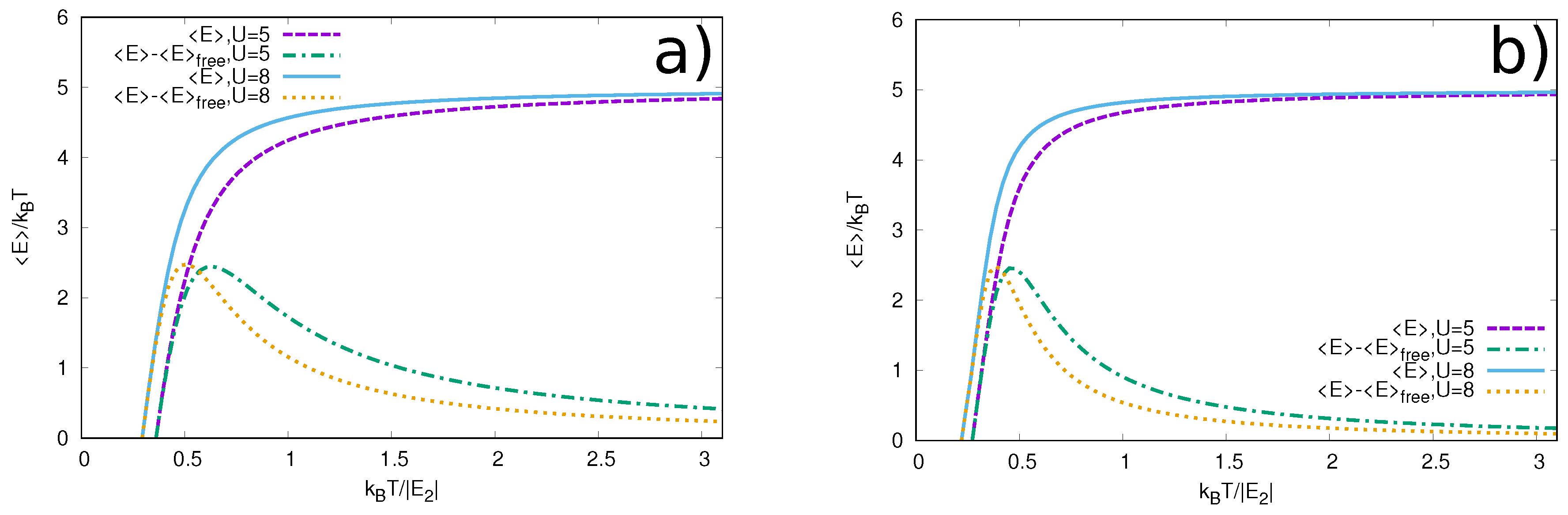
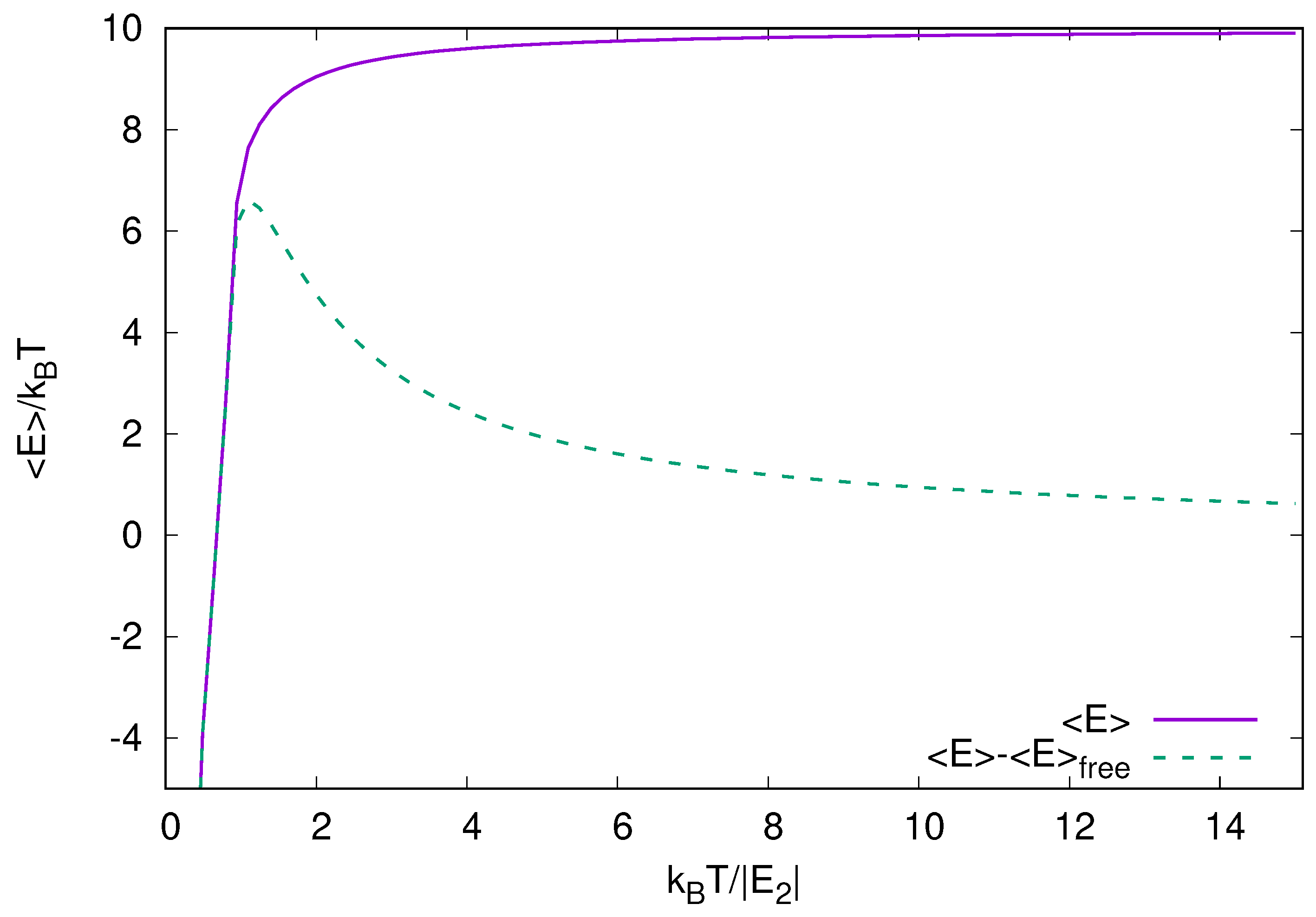
We choose two rather simple systems to be studied in detail as function of temperature. The two systems have five tubes each with either one or two dipoles. We first calculate the temperature dependence of the average energies for different interactions and trap frequencies in comparison with the energies of the free-particle system. These dependencies are all qualitatively the same, i.e., changing from bound-state values to high-temperature statistical equilibrium values. However, finer details reveal weak dependence on the strength of interaction and the trapping frequency.

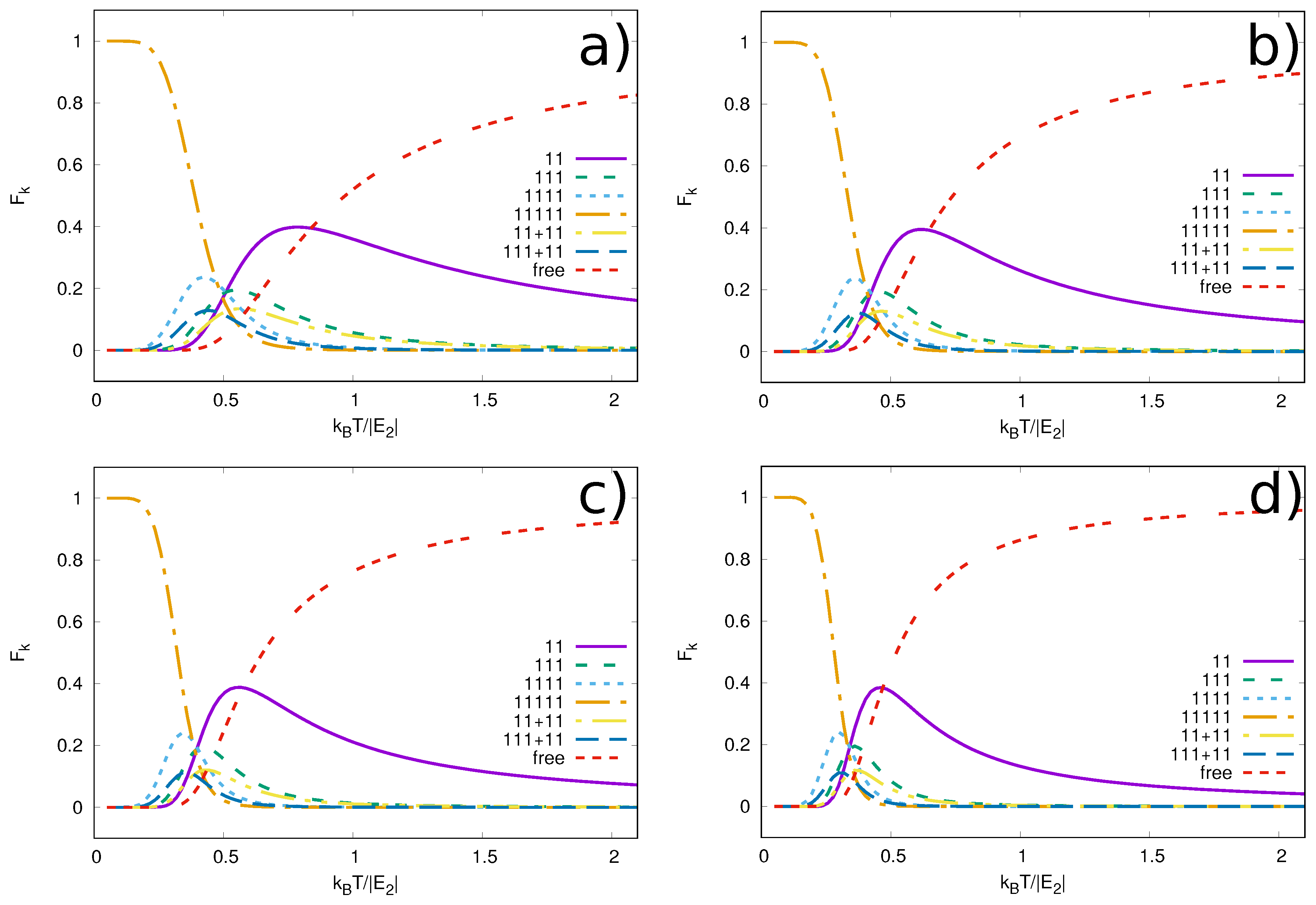
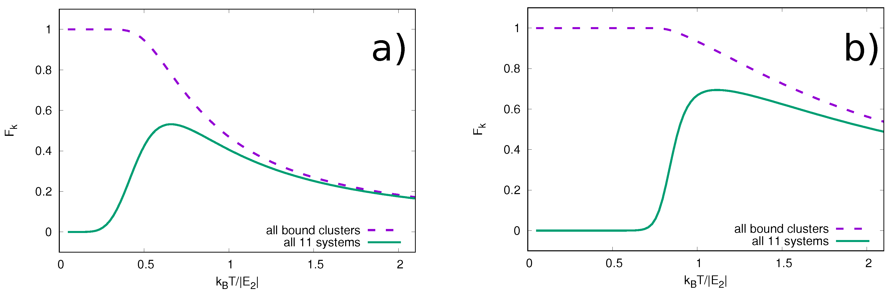
The number of different cluster configurations is relatively large even for the simple systems we choose to study here. The more detailed results of individual cluster occupancies are available through the partition function. We obtain the occupancies of the clusters by increasing the temperature from zero to much higher than the energy of a dimer formed by two dipoles in adjacent layers. These occupancies show a change of the system from the corresponding ground state towards entirely free particles. However, the details of this melting at moderate temperatures reveal how this process proceeds through intermediate configurations of various clusters. At temperatures around the dimer energy the configurations in the ensemble are mixed more than at any other temperature. Our findings show that even though there are many few-body clusters, most of them are unlikely to be detected in a many-body system. Indeed, the system shows a fast transition from a many-body state at low temperatures to a high-temperature state where only the simplest clusters (e.g., a dimer) play a role. This observation suggests that effective theories that include only free particles and dimers can accurately describe the system down to $T\simeq |E_2|/k_B$.

In conclusion, we have presented a method and derived results for the melting of one-dimensional systems of relatively few dipoles. The cluster structures are clearly very important in systems of many particles at moderate temperatures. This suggests a tool for investigating the transition from few- to many physics by changing the temperature in cold-atom systems.

In the future, it will be interesting to extend our results to more complicated systems that could have more particles and/or more tubes. For a more realistic calculation one should include a short-range intra-layer repulsive interaction even for dipoles at a “magic angle”. This interaction will decrease the probability to observe few-body structures that have more than one dipole per layer. Please note that an inclusion of a short-range interaction in Equation (4) with at most two particles per layer still leads to a solvable model [37]. One could study as well two-dimensional systems of layers of particles, which are known to support various few-body bound states [42,43,44]. To increase the probability to observe non-chain few-body clusters, one should again consider tilting dipoles. It is impossible to find an angle that turns off completely the dipole-dipole interaction in a two-dimensional layer, which significantly complicates the problem.

References

1. Efimov, V. Energy levels arising from resonant two-body forces in a three-body system. Phys. Lett. B 1970, 33, 563. [Google Scholar] [CrossRef]
2. Jensen, A.S.; Riisager, K.; Fedorov, D.V.; Garrido, E. Structure and reactions of quantum halos. Rev. Mod. Phys. 2004, 76, 215. [Google Scholar] [CrossRef]
3. Braaten, E.; Hammer, H.W. Universality in few-body systems with large scattering length. Phys. Rep. 2006, 428, 259. [Google Scholar] [CrossRef] [Green Version]
4. Greene, C.H.; Giannakeas, P.; Pérez-Rios, J. Universal few-body physics and cluster formation. Rev. Mod. Phys. 2017, 89, 035006. [Google Scholar] [CrossRef] [Green Version]
5. Naidon, P.; Endo, S. Efimov physics: A review. Rep. Prog. Phys. 2017, 80, 056001. [Google Scholar] [CrossRef] [Green Version]
6. Kraemer, T.; Mark, M.; Waldburger, P.; Danzl, J.G.; Chin, C.; Engeser, B.; Lange, A.D.; Pilch, K.; Jaakkola, A.; Nägerl, H.-C.; et al. Evidence for Efimov quantum states in an ultracold gas of caesium atoms. Nature 2006, 440, 315. [Google Scholar] [CrossRef] [Green Version]
7. Lahaye, T.; Menotti, C.; Santos, L.; Lewenstein, M.; Pfau, T. The physics of dipolar bosonic quantum gases. Rep. Prog. Phys. 2009, 72, 126401. [Google Scholar] [CrossRef]
8. Baranov, M.A.; Dalmonte, M.; Pupillo, G.; Zoller, P. Condensed matter theory of dipolar quantum gases. Chem. Rev. 2012, 112, 5012. [Google Scholar] [CrossRef] [Green Version]
9. Bohn, J.L.; Rey, A.M.; Ye, J. Cold molecules: Progress in quantum engineering of chemistry and quantum matter. Science 2017, 357, 1002. [Google Scholar] [CrossRef] [Green Version]
10. Bloch, I.; Dalibard, J.; Zwerger, W. Many-body physics with ultracold gases. Rev. Mod. Phys. 2008, 80, 885. [Google Scholar] [CrossRef] [Green Version]
11. Wang, D.W.; Lukin, M.D.; Demler, E. Quantum fluids of self-assembled chains of polar molecules. Phys. Rev. Lett. 2006, 97, 180413. [Google Scholar] [CrossRef] [PubMed] [Green Version]
12. Volosniev, A.G.; Armstrong, J.R.; Fedorov, D.V.; Jensen, A.S.; Valiente, M.; Zinner, N.T. Bound states of dipolar bosons in one-dimensional systems. New J. Phys. 2013, 15, 043046. [Google Scholar] [CrossRef]
13. Wunsch, B.; Zinner, N.T.; Mekhov, I.B.; Huang, S.J.; Wang, D.W.; Demler, E. Few-body bound states in dipolar gases and their detection. Phys. Rev. Lett. 2011, 107, 073201. [Google Scholar] [CrossRef] [PubMed] [Green Version]
14. Zinner, N.T.; Wunsch, B.; Mekhov, I.B.; Huang, S.J.; Wang, D.W.; Demler, E. Few-body bound complexes in one-dimensional dipolar gases and nondestructive optical detection. Phys. Rev. A 2011, 84, 063606. [Google Scholar] [CrossRef] [Green Version]
15. Bjerlin, J.; Bengtsson, J.; Deuretzbacher, F.; Kristinsdóttir, L.H.; Reimann, S.M. Dipolar particles in a double-trap confinement: Response to tilting the dipolar orientation. Phys. Rev. A 2018, 97, 023634. [Google Scholar] [CrossRef] [Green Version]
16. Dalmonte, M.; Zoller, P.; Pupillo, G. Trimer liquids and crystals of polar molecules in coupled wires. Phys. Rev. Lett. 2011, 107, 163202. [Google Scholar] [CrossRef] [Green Version]
17. Pikovski, A.; Klawunn, M.; Shlyapnikov, G.V.; Santos, L. Interlayer superfluidity in bilayer systems of fermionic polar molecules. Phys. Rev. Lett. 2010, 105, 215302. [Google Scholar] [CrossRef] [Green Version]
18. Capogrosso-Sansone, B.; Kuklov, A.B. Superfluidity of flexible chains of polar molecules. J. Low Temp. Phys. 2011, 165, 213. [Google Scholar] [CrossRef]
19. Cinti, F.; Wang, D.W.; Boninsegni, M. Phases of dipolar bosons in a bilayer geometry. Phys. Rev. A 2017, 95, 023622. [Google Scholar] [CrossRef] [Green Version]
20. Sinha, S.; Santos, L. Cold dipolar gases in quasi-one-dimensional geometries. Phys. Rev. Lett. 2007, 99, 140406. [Google Scholar] [CrossRef] [Green Version]
21. Deuretzbacher, F.; Cremon, J.C.; Reimann, S.M. Ground-state properties of few dipolar bosons in a quasi-one-dimensional harmonic trap. Phys. Rev. A 2010, 81, 063616. [Google Scholar] [CrossRef] [Green Version]
22. Armstrong, J.R.; Zinner, N.T.; Fedorov, D.V.; Jensen, A.S. Analytic harmonic approach to the N-body problem. J. Phys. B: At. Molecular 2011, 44, 055303. [Google Scholar] [CrossRef] [Green Version]
23. Landau, L.D.; Lifschitz, E.M. Quantum Mechanics: Non-Relativistic Theory, 3rd ed.; Elsevier Butterworth-Heinemann: Amsterdam, The Netherlands, 1977. [Google Scholar]
24. Simon, B. The bound state of weakly coupled Schrodinger operators in one and two dimensions. Ann. Phys. 1976, 97, 279. [Google Scholar] [CrossRef]
25. Armstrong, J.R.; Zinner, N.T.; Fedorov, D.V.; Jensen, A.S. Layers of cold dipolar molecules in the harmonic approximation. Eur. Phys. J. D 2012, 66, 85. [Google Scholar] [CrossRef]
26. McGuire, J.B. Study of exactly soluble one-dimensional N-body problems. J. Math. Phys. 1964, 5, 622. [Google Scholar] [CrossRef]
27. De Palo, S.; Citro, R.; Orignac, E. Variational Bethe ansatz approach for dipolar one-dimensional bosons. Phys. Rev. B 2020, 101, 045102. [Google Scholar] [CrossRef] [Green Version]
28. Kora, Y.; Boninsegni, M. Dipolar bosons in one dimension: The case of longitudinal dipole alignment. Phys. Rev. A 2020, 101, 023602. [Google Scholar] [CrossRef] [Green Version]
29. Oldziejewski, R.; Górecki, W.; Pawłowski, K.; Rzazewski, K. Strongly correlated quantum droplets in quasi-1D dipolar Bose gas. Phys. Rev. Lett. 2020, 124, 090401. [Google Scholar] [CrossRef] [Green Version]
30. Tanzi, L.; Lucioni, E.; Fama, F.; Catani, J.; Fioretti, A.; Gabbanini, C.; Bisset, R.N.; Santos, L.; Modugno, G. Observation of a dipolar quantum gas with metastable supersolid properties. Phys. Rev. Lett. 2019, 122, 130405. [Google Scholar] [CrossRef] [Green Version]
31. Böttcher, F.; Schmidt, J.N.; Wenzel, M.; Hertkorn, J.; Guo, M.; Langen, T.; Pfau, T. Transient supersolid properties in an array of dipolar quantum droplets. Phys. Rev. X 2019, 9, 011051. [Google Scholar] [CrossRef] [Green Version]
32. Chomaz, L.; Petter, D.; Ilzhöfer, P.; Natale, G.; Trautmann, A.; Politi, C.; Durastante, G.; van Bijnen, R.M.W.; Patscheider, A.; Sohmen, M.; et al. Long-lived and transient supersolid behaviors in dipolar quantum gases. Phys. Rev. X 2019, 9, 021012. [Google Scholar] [CrossRef] [Green Version]
33. Böttcher, F.; Wenzel, M.; Schmidt, J.N.; Guo, M.; Langen, T.; Ferrier-Barbut, I.; Pfau, T.; Bombin, R.; Sanchez-Baena, J.; Boronat, J.; et al. Dilute dipolar quantum droplets beyond the extended Gross-Pitaevskii equation. Phys. Rev. Res. 2019, 1, 033088. [Google Scholar] [CrossRef] [Green Version]
34. Karwowski, J. A separable model of N interacting particles. Int. J. Quantum Chem. 2008, 108, 2253. [Google Scholar] [CrossRef]
35. Karwowski, J.; Szewc, K. Separable N-particle Hookean models. J. Phys. Conf. Ser. 2010, 213, 012016. [Google Scholar] [CrossRef]
36. Volosniev, A.G.; Jensen, A.S.; Harshman, N.L.; Armstrong, J.R.; Zinner, N.T. A solvable model for decoupling of interacting clusters. EPL (Europhys. Lett.) 2019, 125, 20003. [Google Scholar] [CrossRef] [Green Version]
37. Armstrong, J.R.; Volosniev, A.G.; Fedorov, D.V.; Jensen, A.S.; Zinner, N.T. Analytic solutions of topologically disjoint systems. J. Phys. A Math. Theor. 2015, 48, 085301. [Google Scholar] [CrossRef] [Green Version]
38. Suzuki, Y.; Varga, K. Stochastic Variational Approach to Quantum-Mechanical Few-Body Problems; Springer: Berlin, Germany, 1998. [Google Scholar]
39. Mitroy, J.; Bubin, S.; Horiuchi, W.; Suzuki, Y.; Adamowicz, L.; Cencek, W.; Szalewicz, K.; Komasa, J.; Blume, D.; Varga, K. Theory and application of explicitly correlated Gaussians. Rev. Mod. Phys. 2013, 85, 693. [Google Scholar] [CrossRef] [Green Version]
40. Busch, T.; Englert, B.-G.; Rzaźewski, K.; Wilkens, M. Two cold atoms in a harmonic trap. Found. Phys. 1998, 28, 549. [Google Scholar] [CrossRef]
41. Dehkharghani, A.S.; Volosniev, A.G.; Zinner, N.T. Impenetrable mass-imbalanced particles in one-dimensional harmonic traps. J. Phys. B At. Mol. Opt. Phys. 2016, 49, 085301. [Google Scholar] [CrossRef]
42. Klawunn, M.; Pikovski, A.; Santos, L. Two-dimensional scattering and bound states of polar molecules in bilayers. Phys. Rev. A 2010, 82, 044701. [Google Scholar] [CrossRef] [Green Version]
43. Volosniev, A.G.; Fedorov, D.V.; Jensen, A.S.; Zinner, N.T. Model independence in two dimensions and polarized cold dipolar molecules. Phys. Rev. Lett. 2011, 106, 250401. [Google Scholar] [CrossRef] [PubMed] [Green Version]
44. Guijarro, G.; Astrakharchik, G.E.; Boronat, J.; Bazak, B.; Petrov, D.S. Few-body bound states of two-dimensional bosons. arXiv 2019, arXiv:1911.01701. [Google Scholar]
Figure 1. The system of interest is five one-dimensional tubes filled with two dipolar particles with dipole moments aligned at the so-called “magic angle”. The system is in a thermal equilibrium with a bath at temperature T. At high temperatures, the system will consist of a gas of independent particles, and at zero temperature the attraction between the layers will lead to a certain bound structure. At intermediate temperatures, various few-body clusters will form.
Mathematics 08 00484 g001
Figure 2. The interaction potential between adjacent tubes at the “magic angle” ϕ = ϕ m (see the text for the definition of the angle). The potential is given by Equation (3) with n = 1 and ϕ = ϕ m : V d i p = U ( d 2 + 2 2 x d ) / ( d 2 + x 2 ) 5 / 2 .
Mathematics 08 00484 g002
Figure 3. Comparison between the harmonic oscillator (HO) model and the stochastic variational method (SVM) in obtaining energies for few-body dipolar clusters. The solid curves represent the results of the HO model: the upper curve is for the 12 system, the lower is for the 111 system. The dots are the corresponding SVM results. The 111 system is slightly more bound than 12 system due to an additional attraction between the outer layers. For comparison, we also plot the energy of the 11 system (see the upper dotted curve) whose energy, by construction, is the same in the HO and SVM calculations. The lower dotted curve presents two times the energy of the 11 system.
Mathematics 08 00484 g003
Figure 4. A figure to illustrate Equation (16). This specific configuration has five free particles, and two clusters. The energy of each cluster consists of two parts: The binding energy, which is calculated as in Section 2, and the center-of-mass part, which is determined by the confining harmonic oscillator.
Mathematics 08 00484 g004
Figure 5. This plot shows the energy of the one-particle-per-layer system, E , and the difference of the energy with the energy of the system of completely free particles, E E f r e e . Panel (a) shows curves for different U with oscillator length values being twice the inter-layer distance, and in panel (b) the oscillator length is 10 the inter-layer distance. The energy curves all start at large negative energies because of the finite binding energy at low temperatures, then approach the high-temperature limit of 5 k B T (the equipartition of energy limit for this system). The curves showing the difference of energies start to separate from the energy curve at k B T / E 2 0.25 to 0.4 as the free-particle state becomes populated before rapidly turning over and descending towards the high-temperature limit of 0.
Mathematics 08 00484 g005
Figure 6. Fractional occupancies of different clusters as a function of temperature for a system of five 1D layers each with one particle. (a): The confining frequency is chosen such that the oscillator length in the tubes is equal to twice the inter-layer distance. The dipole strength is U = 5 . (b): The confining frequency is chosen such that the oscillator length in the tubes is equal to twice the inter-layer distance. The dipole strength is U = 8 . (c) The dipole strength is U = 5 , and the confining frequency is chosen such that the oscillator length in the tubes is equal to 10 the inter-layer distance. (d): The dipole strength is U = 8 and the confining frequency is that same as in panel (c).
Mathematics 08 00484 g006
Figure 7. This plot shows the same as in Figure 5, but for two-particle-per-layer system. The energy curve again starts at large negative energies, then approaches the high-temperature limit of 10 k B T (the equipartition limit for 10 total particles in 1D harmonic potentials). The curve showing the difference of energies starts to separate from the energy curve at k B T / E 2 1 as the free-particle state becomes populated before rapidly turning over and descending towards the high-temperature limit of 0. In contrast with the single particle per layer system, the high-temperature limits are achieved much more slowly. The interaction strength for this plot was U = 5 .
Mathematics 08 00484 g007
Figure 8. (a) Fractional occupancies of all the clusters as a function of temperature for a system of five 1D layers each with two particles. The dipole strength is U = 5 , and the confining frequency is chosen such that the oscillator length in the tubes is equal to twice inter-layer distance. The clusters are labeled by their layer occupancy, so a cluster consisting of one particle each in adjacent layers would be labeled ‘11’. (b) Fractional occupancies of the most populated of the most bound clusters as a function of temperature for a system of five 1D layers each with two particles. The dipole strength is U = 5 , and the confining frequency is chosen such that the oscillator length in the tubes is equal to twice the inter-layer distance. Pictures of the clusters can be seen in (c). (d) Fractional occupancies of the least bound clusters as a function of temperature for a system of five 1D layers each with two particles. The dipole strength is U = 5 , and the confining frequency is chosen such that the oscillator length in the tubes is equal to twice the inter-layer distance. (e) Pictures of the different smaller clusters with the lowest binding energies.
Mathematics 08 00484 g008
Figure 9. This figure shows the fraction of states with at least one bound cluster of any kind (‘all bound clusters’) or the sum of all clusters that contain at least one 11-cluster (all 11 systems). The dipole strength is U = 5 , and the confining frequency is chosen such that the oscillator length in the tubes is equal to twice the inter-layer distance. Panel (a) shows the one-particle-per-layer system and panel (b) shows the two-particle-per-layer system.
Mathematics 08 00484 g009