Abstract
The main aim of this paper is to suggest an algorithm for constructing two monotone sequences of mild lower and upper solutions which are convergent to the mild solution of the initial value problem for Riemann-Liouville fractional delay differential equation. The iterative scheme is based on a monotone iterative technique. The suggested scheme is computerized and applied to solve approximately the initial value problem for scalar nonlinear Riemann-Liouville fractional differential equations with a constant delay on a finite interval. The suggested and well-grounded algorithm is applied to a particular problem and the practical usefulness is illustrated.
1. Introduction
Fractional differential operators are applied successfully to model various processes with anomalous dynamics in science and engineering [1,2]. At the same time, only a small number of fractional differential equations could be solved explicitly. It requires the application of different approximate methods for solving nonlinear factional equations.
This paper deals with an initial value problem for a nonlinear scalar Riemann-Liouville (RL) fractional differential equation with a delay on a closed interval is studied. Mild lower and mild upper solutions are defined. An algorithm for constructing two convergent monotone functional sequences , are given. It is proved both sequences and are the mild minimal and the mild maximal solutions of the given problem. The uniform convergence of both sequences is proved. A special computer program is built and applied to solve particular problems and to illustrate the practical application of the suggested schemes.
Note the monotone iterative techniques combined with lower and upper solutions are applied in the literature to solve various problems in ordinary differential equations [3], differential equations with maxima [4], difference equations with maxima [5], Caputo fractional differential equations [6], Riemann-Liouville fractional differential equations [7,8,9,10].
In this paper, we consider an initial value problem for a scalar nonlinear Riemann-Liouville fractional differential equation with a constant delay on a finite interval. We apply the method of lower and upper solutions and monotone-iterative technique to suggest an algorithm for approximate solving of the studied problem. The suggested and well-grounded algorithm is used in an appropriate computer environment and it is applied to a particular problem to illustrate the practical usefulness.
2. Preliminary and Auxiliary Results
Let be a given function and be a fixed number. Then the Riemann- Liouville fractional derivative of order is defined by (see, for example, [2]
We will give RL fractional derivatives of some elementary functions which will be used later:
Proposition 1.
Reference [2] the following equalities are true:
Consider the initial value problem (IVP) for the nonlinear Riemann-Liouville delay fractional differential equation (FrDDE)
where , , with , N is a natural number, and is a given number.
The solution of the IVP (1) could have a discontinuity at .
Denote the interval
Denote
where are real numbers.
Define the norm in by
Consider the linear scalar delay RL fractional equation of the type
where are real constant, . There exits an explicit formula for the solution of (2) given by see [11]:
where is the Mittag-Leffler function with two parameters.
Note that the solution in the simplest linear case is not easy to obtain. It requires the application of some approximate methods.
Similar to References [12], we have the following result:
Proposition 2.
Let , , be constants and
Then
Similar to References [7], we define the mild solutions:
Definition 1.
The function is a mild solution of the IVP for FrDDE (1), if it satisfies
Remark 1.
Note that the mild solution of the IVP for FrDDE (1) might not be from and it might not have the fractional derivative .
Definition 2.
The function is a mild maximal solution (a mild minimal solution) of the IVP for FrDDE (1), if it is a mild solution of (1) and for any mild solution of (1) the inequality () holds on I and .
3. Mild Lower and Mild Upper Solutions of FrDDE
Definition 3.
The function is a mild lower (a mild upper) solution of the IVP for FrDDE (1), if it satisfies the integral inequalities
and .
Definition 4.
We say that the function is a lower (an upper) solution of the IVP for FrDDE (1), if
Remark 2.
A function could be a mild lower solution or a mild upper solution, respectively, of the IVP for FrDDE (1) but it could not be a lower solution or an upper solution, respectively, of the IVP for FrDDE (1).
Remark 3.
Note that the mild lower solution (mild upper solution) is not unique. At the same time, because of the inequalities in (5) it is much easier to obtain at least one mild lower solution (mild upper solution) than a mild solution of the IVP for FrDDE (1).
4. Monotone-Iterative Techniques for FrDDE
Now we will consider a nonlinear RL fractional differential equation with a constant delay. We will apply a monotone iterative technique to obtain approximate solution. The idea of the formulas for the successive approximations is based on linear RL-fractional differential equations of type (2) and its explicit formula for the solution obtained in [11].
For any two and the constants define the operator (the values of the constants will be defined later):
Theorem 1.
Let the following conditions be fulfilled:
- Let the functions be a lower solution and an upper solution, respectively, of the IVP for FrDDE (1) such that for and , for .
- The function and there exist constants and such that for any the inequality holds.
Then there exist two sequences of functions and , , such that:
- a.
- The sequences and are defined by andthat is,where the constants are defined in condition 2.
- b.
- The sequence is increasing, that is, for .
- c.
- The sequence is decreasing, that is, for , .
- d.
- The inequalityholds.
- e.
- The sequences and converge uniformly on and , on .
- f.
- The limit functions and are mild solutions of the IVP for FrDDE (1) on .
- g.
- The inequalities hold on for any .
Proof of Theorem 1.
Let be a lower solution of the IVP for FrDDE (1), that is,
where
According to Proposition 2, the inequality
holds.
Let and for
We use induction w.r.t. the interval to prove properties of the sequences of successive approximations.
From the definition of the operator and equality it follows that for all integers .
Let . From the definition of the operator and inequalities (8) we obtain
From the definition of the operator , condition 2, the inequality (9) and the equality for we get
Similarly, we can prove
and
Let . From the definition of the operator , the inequalities (8) and for we obtain
Also, from condition 2, the inequalities (8) and for we get
Similarly, we can prove
and
Following the induction process w.r.t. the interval we prove the claims (b) and (c).
Now, we will prove the claim (d). Let . From the definition of the operator , condition 2, the inequality (9) we get
Similarly, we can prove
Let . From condition 2, the inequalities (8) and for we obtain we get
Similarly, we can prove
Now consider the sequences and . They are increasing and decreasing, respectively, and bounded. Thus, they are equicontinuous on (the proof is similar to that in [13] and we omit it). Therefore, they are uniformly convergent on . Denote, and According to the above (b), (c) and (d) the inequalities
hold.
From the uniform convergence of the sequences and we have the point-wise convergence of the sequences and on to and , respectively.
Consider the continuous extension of the integral form of on :
Take the limit in (14) and we obtain the Volterra fractional integral equation
or
From equalities according to Proposition 2 applied to Equation (16) the limit function is a solution of the linear FrDDE
Therefore, the function is a solution of the IVP for FrDDE (1).
The proof about is similar.
Proof of claim g). From claim (d) and the inequality (6) it follows that for any fixed and . Then applying claim (e) we get for any fixed . Therefore, for any on . □
5. Application of the Suggested Algorithm
Now we will apply the algorithm suggested in Theorem 1 for approximate obtaining of the solution of nonlinear RL fractional differential equation with a delay. We will use computer realization of this algorithm to obtain the values of the approximate solutions and to graph them.
Example 1.

Let and consider the IVP for scalar nonlinear Riemann-Liouville FrDDE
with , and .
The function
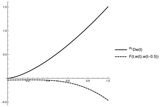
is an upper solution on of the IVP for FrDE (17) since and according to Proposition 1 with and the following inequalities
are satisfied (see Figure 1).
Figure 1.
Graphs of the fractional derivative of the function and the right side part of the equation on .
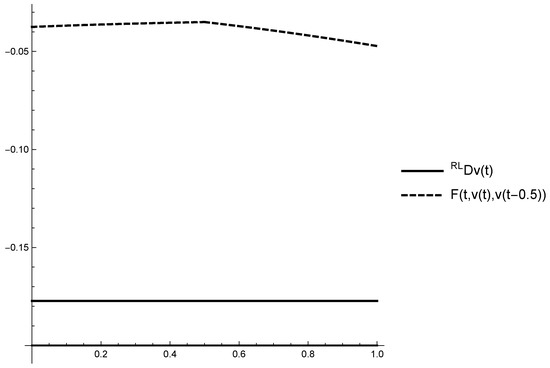
The function
is a lower solution on of the IVP for FrDDE (17) because holds and according to Proposition 1 with the following inequalities
are satisfied (see Figure 2).
Figure 2.
Graphs of the fractional derivative of the functions and the right side part of the equation on .
Note that the lower and upper solutions and are not unique. For example the function
is also an upper solution. But we take just one lower (upper) solution to start the procedure.
Also, the inequality on holds.
For any we have , and therefore,
Applying the inequalities , , and , , we get the inequality with . Therefore, all conditions of Theorem 1 are fulfilled.
We apply the iterative scheme, suggested in Theorem 1, to obtain the successive approximations to the mild solution and to illustrate the claims of Theorem 1.
Define the zero approximation by and for .
Starting from the function we obtain the first lower approximation
the second lower approximation
and so on.
About the upper approximations we start from and obtain the first upper approximation
the second upper approximation
and so on.
The numerical values of the lower/upper approximations, given analytically above, are obtained by a computer program written in C#. We will briefly describe the computerized algorithm for obtaining these successive approximations:
The numerical values of the sequences of successive approximations and , , , are written in two dimensional arrays. The length of any of these arrays depends on the step in the interval .
We calculate in advance the values of the Mittag-Leffler function in the points t, which will be used for numerical solving of the integrals (see Equations (18) and (19)). In the same points we also obtain the values of . These results are written in arrays with lengths, depending on the step on interval . Note that the values of the Mittag-Leffler function are calculated by the help of the main definition (as an infinite sum) with an initially given error.
We use the trapezoid method with an initially given error to solve numerically the integrals of the type for each approximation k and any fixed . The values of both multipliers and are taken from initially formed arrays. Note that it could be used another numerical method for solving the required definite integrals.
For example, to calculate the values of we use the following function
private double Calc_v_t(double[,] v, int k, long it)
{
double f, pf, sum = 0, s = 0, q = 0.5;
long shift = (long)(0.5/eps)+1;
long sh2 = shift/2;
long i = shift, ie = it;
pf = PowTmS[ie] * Eqq[ie] *
((v[k-1,i]*v[k-1,i]+0.05) * (-q+v[k-1,i-sh2]/(s+1)) -
(-v[k-1,i]+0.05*(v[k-1,i-sh2]-v[k,i-sh2])));
while (s < tval)
{
i++; ie--; s += eps;
f = PowTmS[ie] * Eqq[ie] *
((v[k-1,i]*v[k-1,i]+0.05) * (-q+v[k-1,i-sh2]/(s+1)) -
(-v[k-1,i]+0.05*(v[k-1,i-sh2]-v[k,i-sh2])));
sum += (pf + f) * eps;
pf = f;
}
return sum / 2;
}
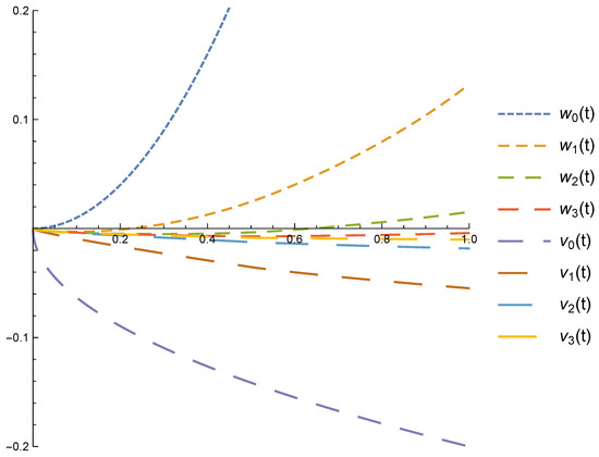
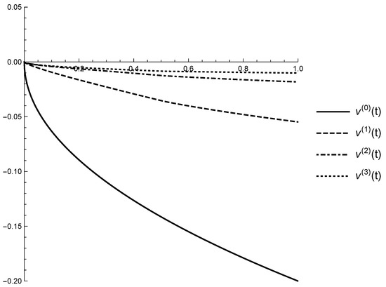
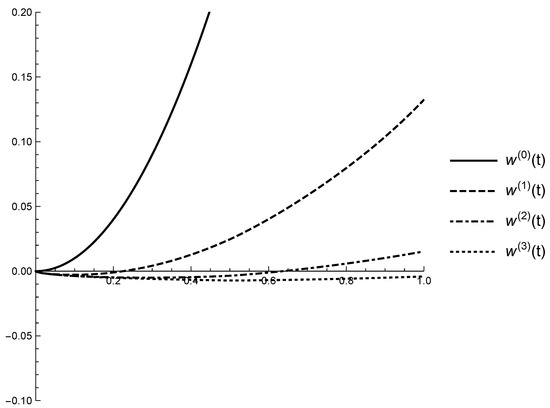
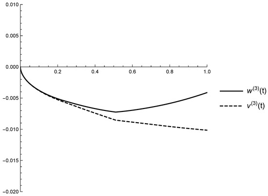
A part of the obtained numerical values of the successive approximations are given in Table 1 and they are used to generate the graphs on Figure 3, Figure 4, Figure 5 and Figure 6).
Table 1.
Values of successive approximations and , for .
Figure 3.
Graphs of the upper/lpwer successive approximations and , , on the interval .
Figure 4.
Graphs of the successive lower approximations , , on the interval .
Figure 5.
Graphs of the successive upper approximations , , on the interval .
Figure 6.
Graphs of the successive approximations and on the interval .
Table 1 and Figure 3, Figure 4, Figure 5 and Figure 6 illustrate the claims of Theorem 1 for the obtained successive approximations:
- -
- -
- -
According to the claim (g) of Theorem 1 the mild solutions and of the FrDDE (17) are between the last obtained lower solution and upper solution . So, practically the suggested algorithm for the approximate solving of IVP for FrDDE gives us a lower and upper bounds of the unknown exact solution.
6. Conclusions
The main aim of the paper is to suggest a scheme for the approximate solving of the initial value problem for scalar nonlinear Riemann-Liouville fractional differential equations with a constant delay on a finite interval. The iterative scheme is based on the method of lower and upper solutions. In connection with this, mild lower and mild upper solutions are defined. An algorithm for constructing two monotone sequences of mild lower and mild upper solutions, respectively, is given. It is proved both sequences are convergent to the exact solution of the studied problem. The iterative scheme is used in a computer environment to illustrate its application for solving a particular nonlinear problem. The suggested and computerized algorithm can be applied to solve approximately and to study the behavior of scalar models with RL fractional derives and delays. The practical application requires the next step in the investigations, more exactly to obtain an algorithm for approximate solving of systems with RL derivatives and delays.
Author Contributions
Conceptualization, S.H.; Methodology, S.H.; Software, A.G. and K.S.; Validation, A.G. and K.S.; Formal Analysis, S.H.; Writing—Original Draft Preparation, S.H., A.G. and K.S.; Writing—Review and Editing, S.H., A.G. and K.S.; Visualization, A.G. and K.S.; Supervision, S.H.; Funding Acquisition, S.H. All authors have read and agreed to the published version of the manuscript.
Funding
S.H. is partially supported by the Bulgarian National Science Fund under Project KP-06-N32/7.
Conflicts of Interest
The authors declare no conflict of interest.
References
- Das, S. Functional Fractional Calculus; Springer: Berlin/Heidelberg, Germany, 2011. [Google Scholar]
- Podlubny, I. Fractional Differential Equations; Academic Press: San Diego, CA, USA, 1999. [Google Scholar]
- Ladde, G.; Lakshmikantham, V.; Vatsala, A. Monotone Iterative Techniques for Nonlinear Differential Equations; Pitman: Boston, MA, USA, 1985. [Google Scholar]
- Hristova, S.; Golev, A.; Stefanova, K. Approximate method for boundary value problems of anti-periodic type for differential equations with “maxima”. Bound. Value Probl. 2013, 2013, 12. [Google Scholar] [CrossRef][Green Version]
- Agarwal, R.; Hristova, S.; Golev, A.; Stefanova, K. Monotone-iterative method for mixed boundary value problems for generalized difference equations with “maxima”. J. Appl. Math. Comput. 2013, 43, 213–233. [Google Scholar] [CrossRef]
- Agarwal, R.; Golev, A.; Hristova, S.; O’Regan, D.; Stefanova, K. Iterative techniques with computer realization for the initial value problem for Caputo fractional differential equations. J. Appl. Math. Comput. 2017. [Google Scholar] [CrossRef]
- Agarwal, R.; Golev, A.; Hristova, S.; O’Regan, D. Iterative techniques with computer realization for initial value problems for Riemann–Liouville fractional differential equations. J. Appl. Anal. 2020. [Google Scholar] [CrossRef]
- Bai, Z.; Zhang, S.; Sun, S.; Yin, C. Monotone iterative method for fractional differential equations. Electron. J. Differ. Equ. 2016, 2016, 1–8. [Google Scholar]
- Denton, Z. Monotone method for Riemann-Liouville multi-order fractional differential systems. Opusc. Math. 2016, 36, 189–206. [Google Scholar] [CrossRef]
- Wang, G.; Baleanu, D.; Zhang, L. Monotone iterative method for a class of nonlinear fractional differential equations. Fract. Calc. Appl. Anal. 2012, 15, 244–252. [Google Scholar] [CrossRef]
- Agarwal, R.; Hristova, S.; O’Regan, D. Explicit solutions of initial value problems for linear scalar Riemann-Liouville fractional differential equations with a constant delay. Mathematics 2020, 8, 32. [Google Scholar] [CrossRef]
- Denton, Z.; Ng, P.; Vatsala, A. Quasilinearization method via lower and upper solutions for Riemann-Liouville fractional differential equations. Nonlinear Dyn. Syst. Theory 2011, 11, 239–251. [Google Scholar]
- Ramırez, J.; Vatsala, A. Monotone iterative technique for fractional differential equations with periodic boundary conditions. Opusc. Math. 2009, 29, 289–304. [Google Scholar] [CrossRef]
© 2020 by the authors. Licensee MDPI, Basel, Switzerland. This article is an open access article distributed under the terms and conditions of the Creative Commons Attribution (CC BY) license (http://creativecommons.org/licenses/by/4.0/).