Article

Long-Range Correlations and Characterization of Financial and Volcanic Time Series

by
Maria C. Mariani
1,*,
Peter K. Asante
2,
Md Al Masum Bhuiyan
2,
Maria P. Beccar-Varela
3,
Sebastian Jaroszewicz
4 and
Osei K. Tweneboah
2
1
Department of Mathematical Sciences and Computational Science Program, University of Texas at El Paso, El Paso, TX 79968-0514, USA
2
Computational Science Program, University of Texas at El Paso, El Paso, TX 79968-0514, USA
3
Department of Mathematical Sciences, University of Texas at El Paso, El Paso, TX 79968-0514, USA
4
Comisión Nacional de Energía Atómica, Buenos Aires, Argentina
*
Author to whom correspondence should be addressed.
Mathematics 2020, 8(3), 441; https://doi.org/10.3390/math8030441
Submission received: 31 January 2020 / Revised: 6 March 2020 / Accepted: 10 March 2020 / Published: 18 March 2020

Abstract

:
In this study, we use the Diffusion Entropy Analysis (DEA) to analyze and detect the scaling properties of time series from both emerging and well established markets as well as volcanic eruptions recorded by a seismic station, both financial and volcanic time series data have high frequencies. The objective is to determine whether they follow a Gaussian or Lévy distribution, as well as establish the existence of long-range correlations in these time series. The results obtained from the DEA technique are compared with the Hurst R/S analysis and Detrended Fluctuation Analysis (DFA) methodologies. We conclude that these methodologies are effective in classifying the high frequency financial indices and volcanic eruption data—the financial time series can be characterized by a Lévy walk while the volcanic time series is characterized by a Lévy flight.

1. Introduction

The collection and analysis of time series data is a very important area of research. Inferences drawn from these data sets have helped in forecasting as well as various industrial product improvements. One important inference usually sought for is whether the time series exhibits persistence (long-range correlations), randomness or anti-persistence. Long-range correlations refers to the slow decay of the temporal or spatial correlation function defined as
γ x y ( δ ) = X ( t ) Y ( t + δ ) .
A time series data which exhibits long-range correlations implies that the evolution of the system is affected by previous system states over long periods of time [1,2,3,4,5]. This makes the need to determine long-range correlations in time series data very important for various fields.
Figure 1 shows the plot of a time series exhibiting a short term and long-term dependency. The plot shows the hourly occupancy rate of a road in the bay area. From the plot we observe two repeating patterns, daily and weekly. The daily describes the morning peaks vs. evening peaks, whereas the weekly reflects the workday and weekend patterns.
However to determine the existence of long-range correlations using the formula in Equation (1) poses challenges due to its sensitivity to noise. This in addition to other factors has pushed research into the development of a number of scaling methods [2,3,4,5,7,8,9,10,11,12,13,14,15,16].
Various scaling methods exist and have been utilized by many researchers in detecting the persistence or anti-persistence in time series. Most notable applications are in financial and geophysical time series. Some examples of these scaling methods are the Rescaled Range Analysis (R/S), the Detrended Fluctuation Analysis (DFA), the Relative Dispersion Analysis (RDA) and the fairly recent Diffusion Entropy Analysis (DEA) which was developed by Scafetta [7,8,9]. Scafetta used the DEA to detect the scaling behavior of DNA sequences. The R/S, DFA, and RDA are examples of variance scaling methods and their scaling exponent is called the Hurst exponent, named after Hurst who first studied it in hydrology while the DEA on the other hand is a pdf scaling method.
The variance scaling methods however encounter various challenges when faced with time series data that exhibit anomalous behaviors. The R/S analysis in particular is usually unable to detect correctly the scaling exponent of non-stationary time series data while the DFA is known to overestimate the scaling exponent. Thus two short comings of these variance scaling methods are their inability to detect the exact value of the exponent though they may be able to detect the scale invariance and their unavailability for processes with infinite variances like the Lévy flight [7].
This is what makes the DEA, our main focus of this paper an important method in detecting the scaling exponent within a time series data. The DEA detects the scaling parameter δ using the pdf of the diffusion process derived from the time series. The advantage of DEA over the variance scaling methods is that it is able to establish the possible existence of scaling in time series data with normal or anomalous properties efficiently without any data alteration due to detrending [7,8,9,17].
Researches focused on long-range correlations have made it possible to gain more insight into long range evolution patterns of complex and chaotic occurrences both in nature (geophysical time series) and other equally important fields including financial markets, traffic analysis, bio engineering, and others. The results from these researches have provided various approaches to minimize risk and forecast or predict future dynamical trends [7,8,9,10,18].
In this study we consider several financial time series data as well as some geophysical time series data and analyze their long-range correlations using R/S analysis, the DFA and the DEA. The continuous time-varying Lévy process is effective for capturing the stochastic volatility (SV) and fat tails of data distribution. It is known that the volatilities of high frequency data are correlated, and they vary stochastically over time. We seek to determine the characterization of the time series data (i.e., whether it follows the Gaussian or Lévy distribution) by comparing the relation between the scaling exponent derived with the R/S and DFA against that of the DEA. This manuscript is organized as follows: A brief background of R/S and DFA and a detailed background of the DEA with the procedure used to detect the scaling exponent ( δ ) for a stationary and non-stationary time series data is presented in Section 2. Section 3 presents an overview of the data including results on stationarity of the series. A table of results and figures are shown in Section 4, and finally Section 5 and Section 6 contain a brief discussion and conclusion.

2. Variance Scaling Methods

In this section we briefly introduce the Rescaled Range Analysis and the Detrended Fluctuation Analysis. The Diffusion Entropy Analysis is then discussed with more detail.

2.1. Rescaled Range Analysis

The idea of the Rescaled-Range analysis (R/S) was presented by Hurst in the framework of his study on the long-run variations of the water level of the Nile river [19]. It has become very popular since then, and has been applied to a wide range of disciplines, including traffic analysis, bioengineering, physics, geology, biology and geophysics [20].
The name H for the parameter derived from this technique was coined by Mandelbrot in tribute to the hydrologist Hurst and the mathematician Holder. The parameter H also known as index of dependence represents the relative trend of a time series and always lies between 0 and 1, it is equal to 1 2 in the case of processes with independent increments. Of particular interest for our work is the case in which 0.5 < H < 1 since it is an indicator of long-range correlations.

2.2. Detrended Fluctuation Analysis

In order to study the self-similarity and long-range dependence of time series Peng et al. [21] proposed the Detrended Fluctuation Analysis (DFA) while examining a series of DNA nucleotides. From the moment it was proposed to date, DFA has become a widely used method for the determination of fractal scaling properties and the detection of long-range correlations in non-stationary time series. It has been applied for example in biology, meteorology, geophysics and economics [21,22,23,24,25,26,27].
The principal advantage of the DFA lies in its ability to differentiate the intrinsic autocorrelations of the time series from those imposed by non-stationary external trends. That is, the method focuses on the intrinsic structure of the correlations of market fluctuations at different time scales, leaving aside non-stationary trends.
The application of the DFA method allows obtaining a scale exponent α from estimating the slope of function F ( s ) that measures the mean square deviation from an optimal linear approximation around the trend signal in segments of length s. The fluctuation function vs s behaves as a power law. Therefore it is possible to compute the value of the exponent α from the slope of the function in a log-log scale plot of F ( s ) vs s. The DFA exponent α and the Hurst parameter H are related by
H = α if 0 < α < 1 α 1 if α 1 .
However, due to its sensitivity to abnormal values in the series, the rescaled range analysis method is not suitable for analyzing long-range auto-correlation for non-stationary series.

2.3. Diffusion Entropy Analysis

Based on the direct evaluation of the Shannon entropy [7,8,9,14,15], the DEA is a pdf scaling method which perceives the numbers in a time series as the trajectory of a diffusion process [13].
The scaling property for the stationary time series takes the form
p ( x , t ) = 1 t δ F ( x t δ ) ,
where x denotes the diffusion variable, p ( x , t ) is its probability density function (pdf) at time t, and 0 < δ < 1 is the scaling exponent.
The scaling property for the non-stationary time series takes the form
p ( x , t ) = 1 t δ ( t ) F ( x t δ ( t ) ) .
As derived in References [7,8], a diffusion process generated by Lévy walk is characterized by the following relation:
δ = 1 3 2 ( H , α ) .
If δ = ( H , α ) , the time series can be characterized by Fractional Brownian Motion (FBM), since the variance methods are based subtly on the Gaussian assumption [1,19]. However if δ ( H , α ) , and the Equation (5) holds true, the noise can be characterized by Lévy statistics. ( H , α ) in Equation (5) refers to the scaling exponent derived from the variance scaling methods.

2.4. Estimation Procedure

In this subsection, we describe the estimation technique for the scaling exponent, δ . We first present a brief background on the Shannon Entropy that is used for estimating δ .

The Shannon Entropy

The concept of entropy was developed by Rudolph Clausius in 1865, a few years after he stated the laws of thermodynamics [18,28]. The entropy is an indicator of the lack of information about the measure of an event that occurs with propability p [18].
Other types of entropies are the Kolmogorov-sinai entropy, the Renyi entropy and the Tsallis entropy [7,8,9,18]. The Shannon entropy (named by Shannon) measures information of a probability distribution as follows:
S ( t ) = 1 N p i log p i .
The summation is replaced by the integral in the case of continuous probability distributions. The above equation is used to derive the log equation that will be used to determine the DEA δ scaling. See below the technique for estimating δ :
  • The time series data is first transformed into a diffusion process.
  • Shannon’s entropy of the diffusion process is calculated. A log-linear equation or log-quadratic equation is derived from the Shannon entropy by substituting Equations (3) and (4) respectively. Simplifying the result from the substitutions, we have the following relation for stationary time series:
    S ( t ) = A + δ l n ( t ) .
    For the non-stationary series, the relation is as follows:
    S ( t ) = A + δ ( t ) τ ,
    where δ ( t ) = δ 0 + η log ( t ) and τ = log ( t ) with η log ( t ) < 1 δ 0 . After some simplifications, Equation (8) becomes
    S ( t ) = A + ( δ 0 K ) log ( t ) + ( 1 δ 0 ) ( log ( t ) ) 2 ,
    where K < 0 and δ 0 δ from the stationary pdf. Thus, by fitting a log-quadratic model in the non-stationary series and a log-linear model in the stationary series we are able to determine the δ ( δ 0 ) scaling. At t = 1 , it is clear that the constant A in both Equations (7) and (8) is given by S ( 1 ) .
    Thus δ (or δ 0 ) is derived by an estimation of the slope of the above linear-log equation or by the coefficients from the quadratic-log equation. For details of the algorithm used when transforming the series into a diffusion process, we refer the reader to Reference [7].

3. Financial and Volcanic Time Series

In this work we have applied two variance scaling methods (R/S analysis and DFA) and a pdf scaling method (DEA) on financial and volcanic time series data. This section gives a brief background of the data sets used and also presents the stationarity test—Augmented Dickey-Fuller test (ADF) was used for checking the time series stationarity [29].

3.1. Financial Time Series

The financial data used was taken from: Mexico (MXX), from 8 November 1991 to 22 October 2001; Brazil (BOVESPA), from 27 April 1993 to 24 June 2005; Argentina (MERVAL), from 8 October 1996 to 24 June 2005; Hong Kong (HSI), from 2 January 1991 to 24 June 2005; Phillipines (PSI), from 1997 to 2001; Thailand (SETI), from 1997 to 2001; New York (SP500) from 3 January 1950 to 23 June 2005; USA (SPC), from 1991 to 2001; Turkey (XU100) from 1997 to 2001 and USA (NASDAQ), from 1997 to 2001.

3.2. Volcanic Time Series

The Volcanic data used was recorded by seismic stations belonging to the Bezymianny Volcano Campaign Seismic Network (PIRE). Data was requested for 10 days before and 5 days after the published time of the volcanic eruptions. The seismic stations used were BEZB and BELO. Volcanic eruptions 1 and 2 were from BEZB and Volcanic eruptions 3–8 were from BELO.

3.3. Stationarity of the Financial and Volcanic Time Series

In this section the stationarity of the Financial and Volcanic data is determined by using the Augmented Dickey-Fuller test (ADF). We implemented both methods in R and Python.

3.3.1. Augmented Dickey-Fuller

The Augmented Dickey-Fuller test is a type of statistical test called unit root test. The null hypothesis of the test is that if the time series can be represented by a unit root, thus it is not stationary (has some time-dependent structure). The alternate hypothesis (rejecting the null hypothesis) is that the time series is stationary.

3.3.2. Financial Time Series

After implementing the ADF test to the financial data the results in Table 1 were obtained for p-values at α = 0.05 .

3.3.3. Volcanic Time Series

After implementing the ADF test to the Volcanic time series the results in Table 2 were obtained for p-values at α = 0.05 .
The above tables summarize the results obtained for the two time series, it is clear from both tests that the volcanic time series is non-stationary while the financial time series is stationary.

4. Results

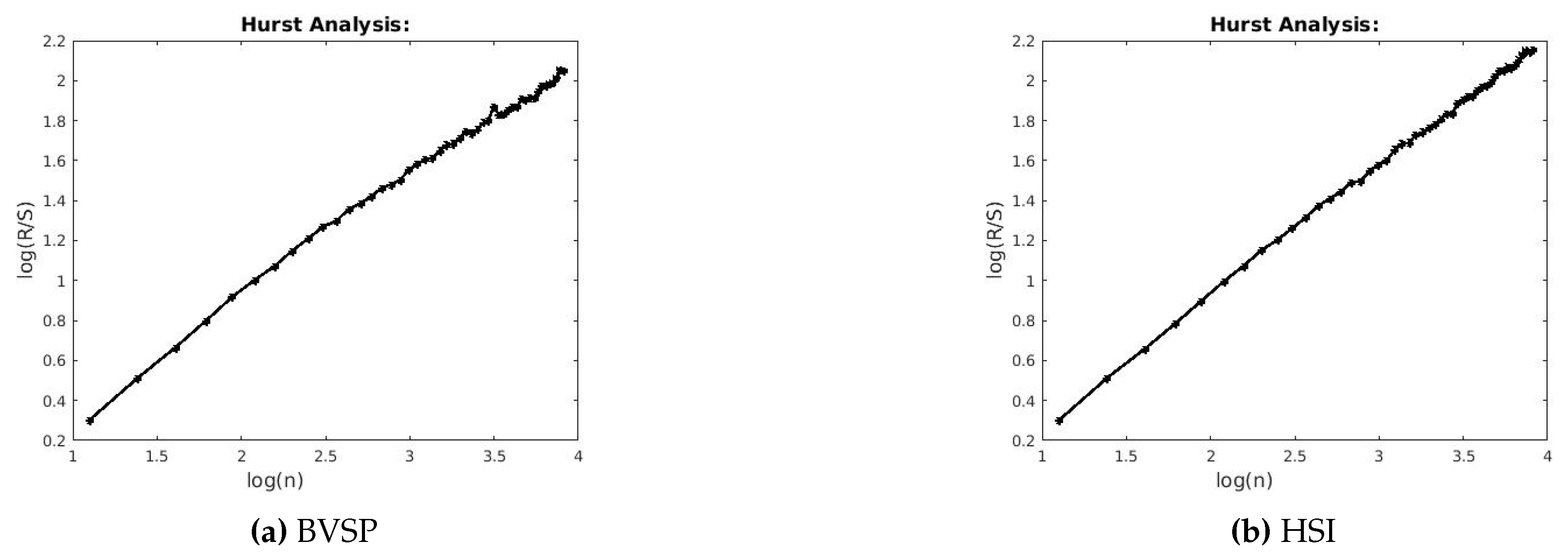
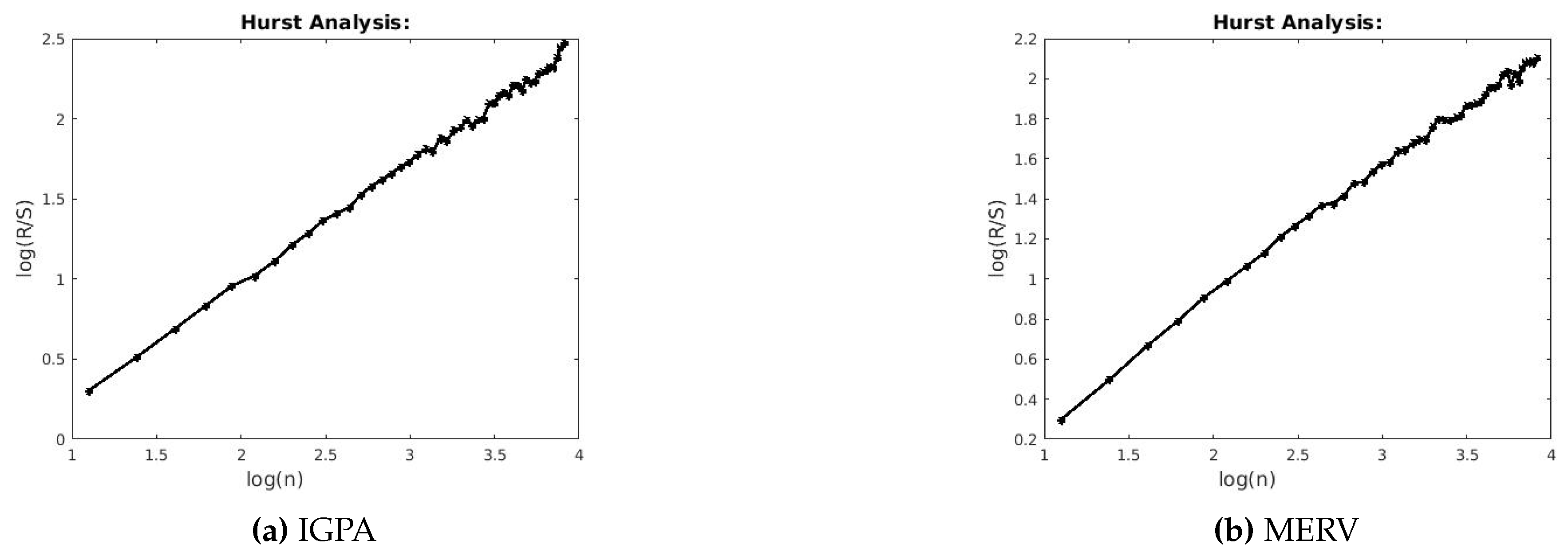
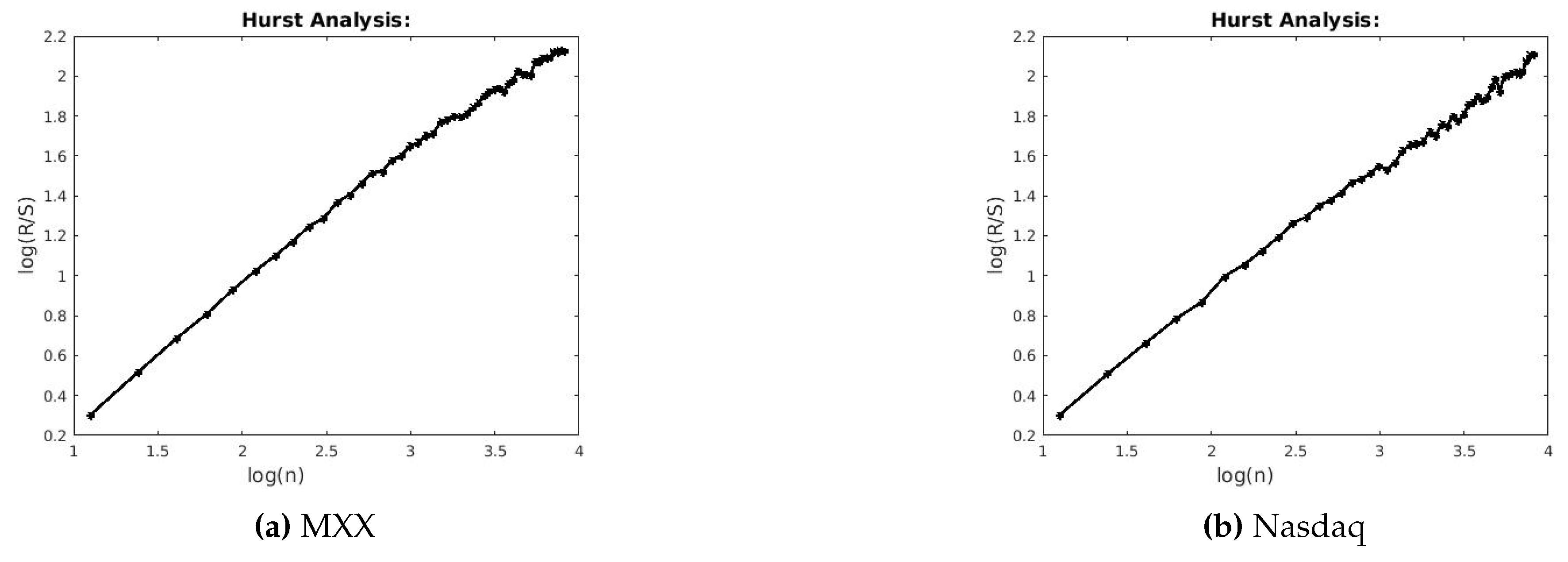
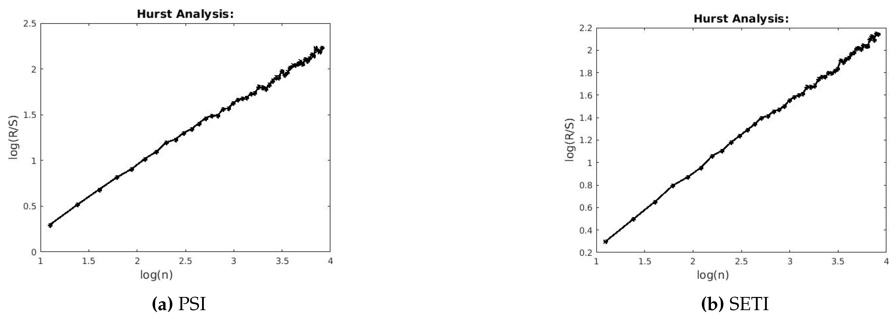
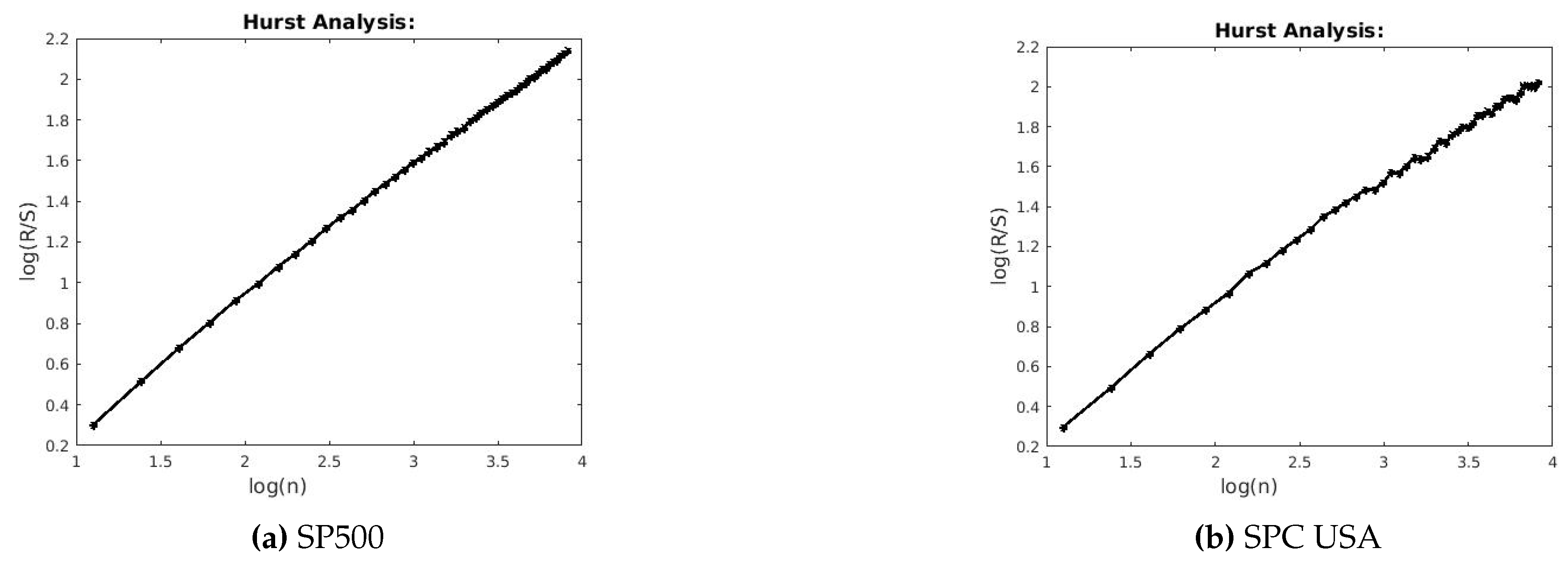
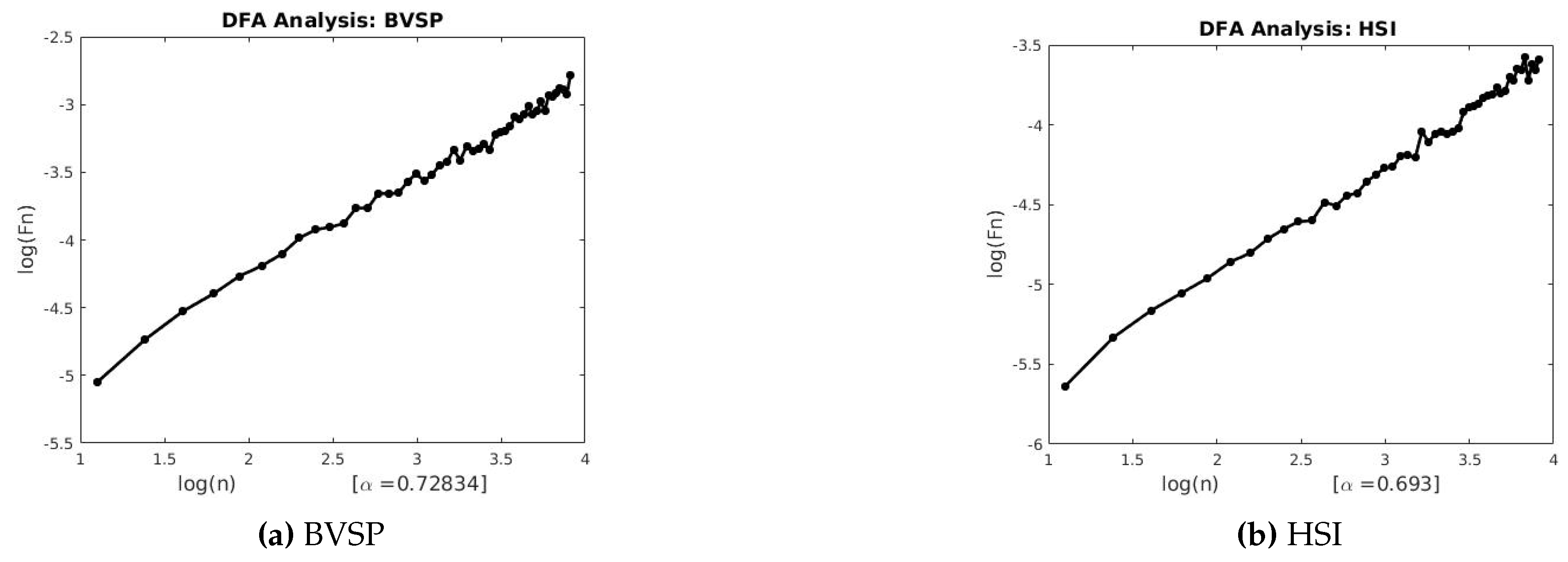
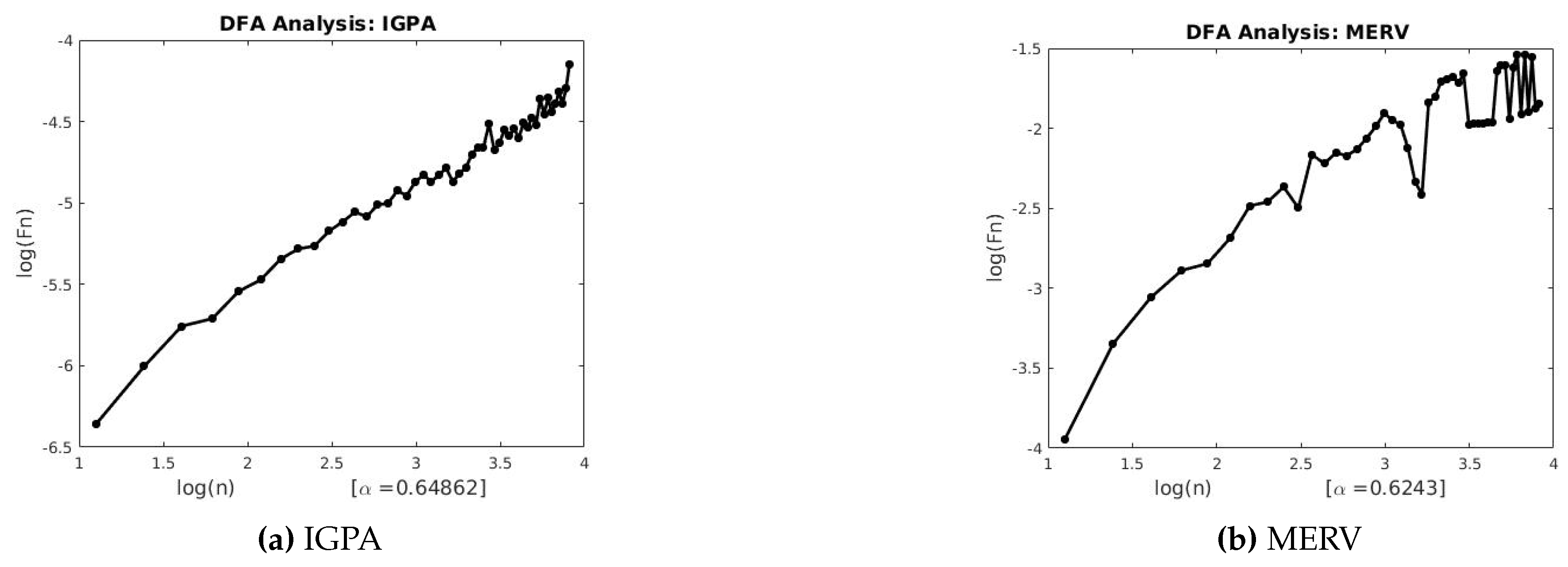
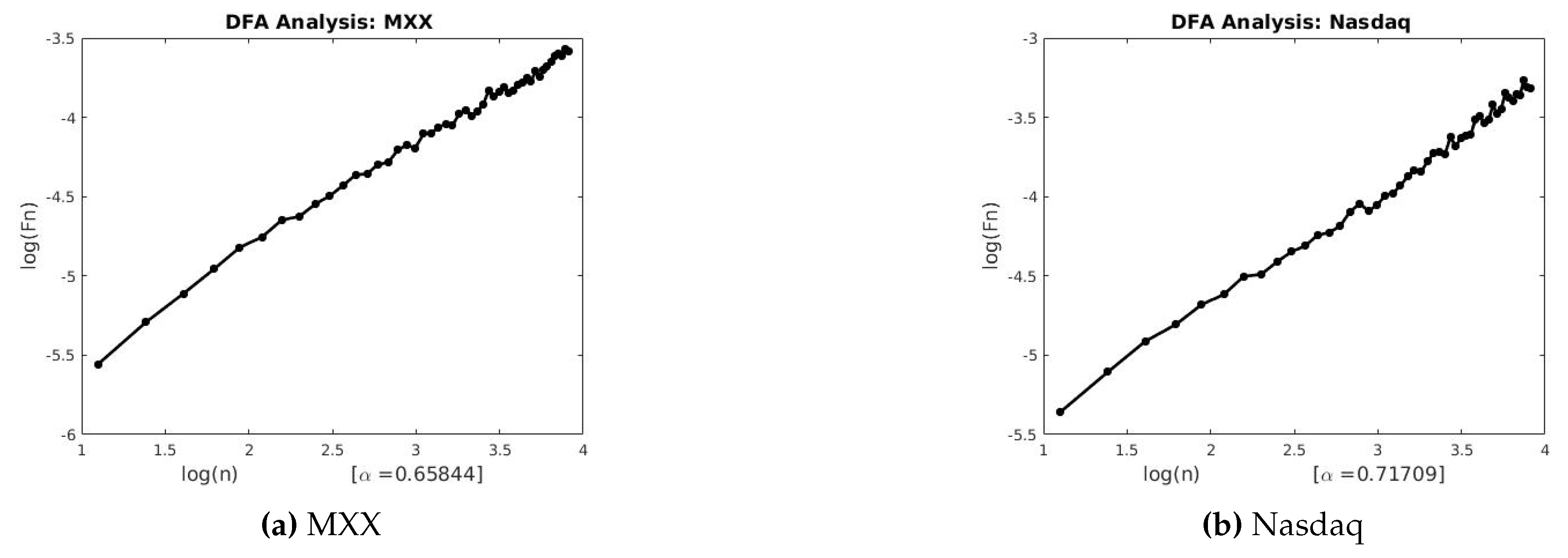
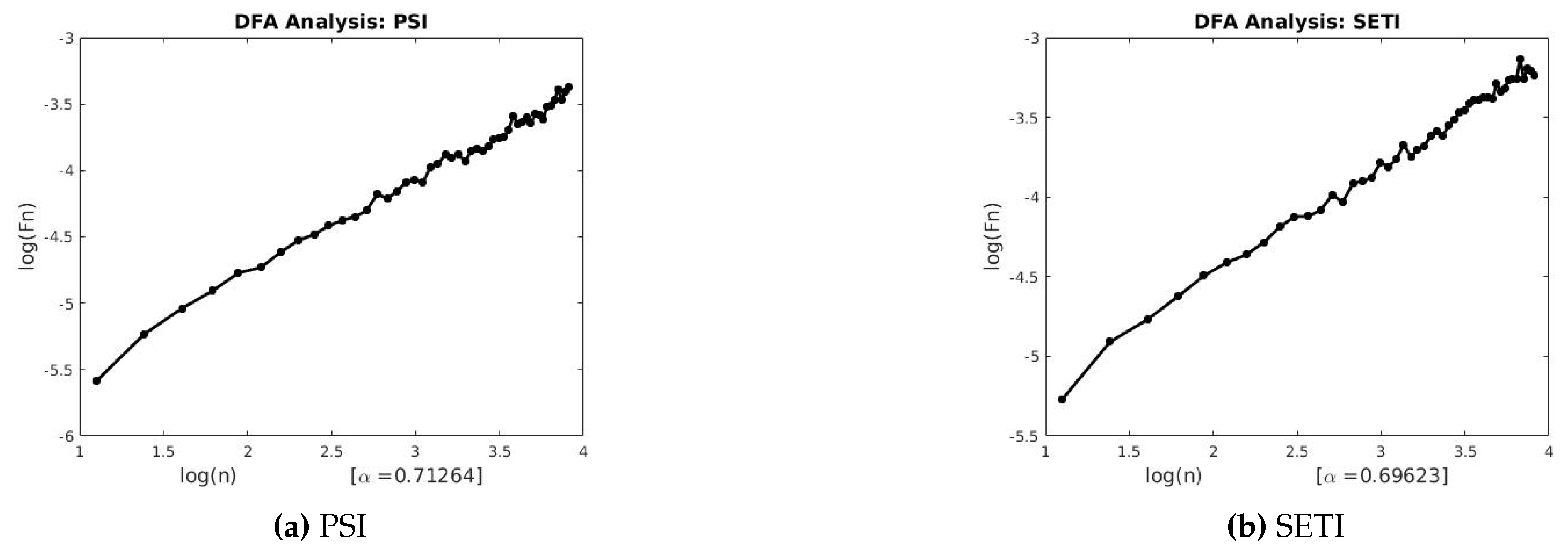
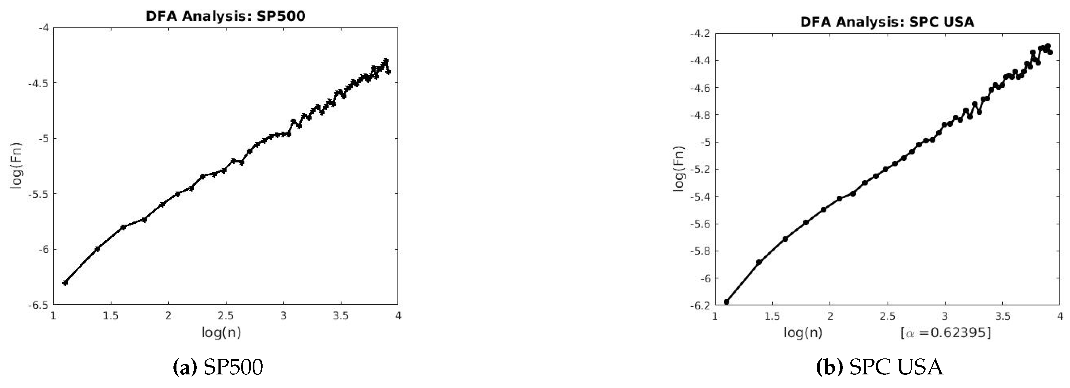
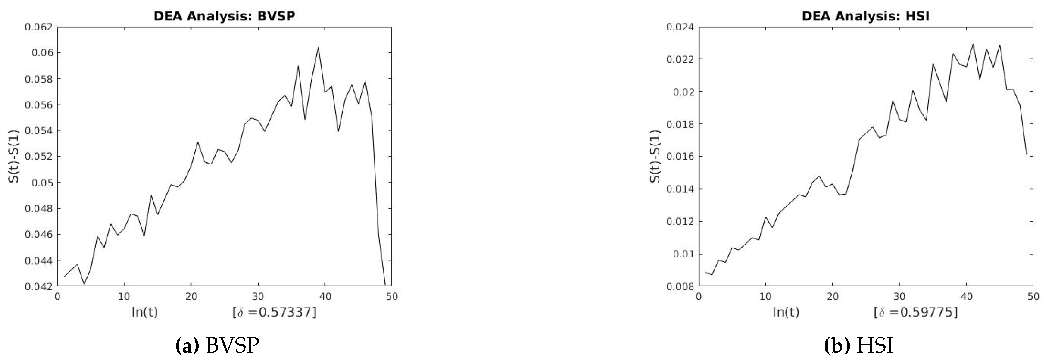
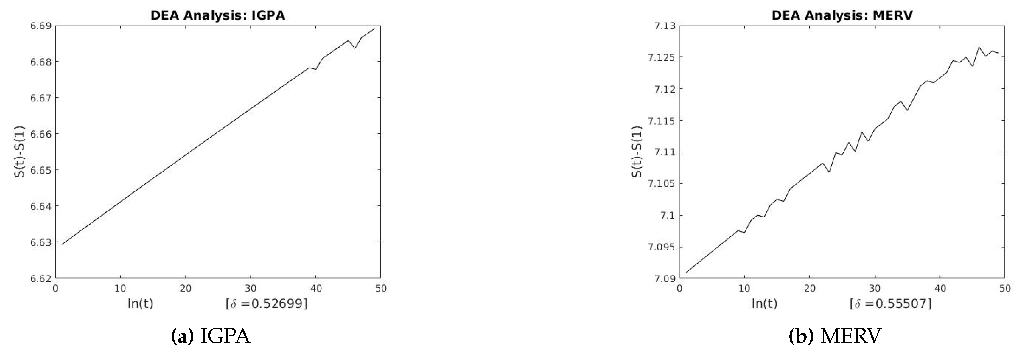
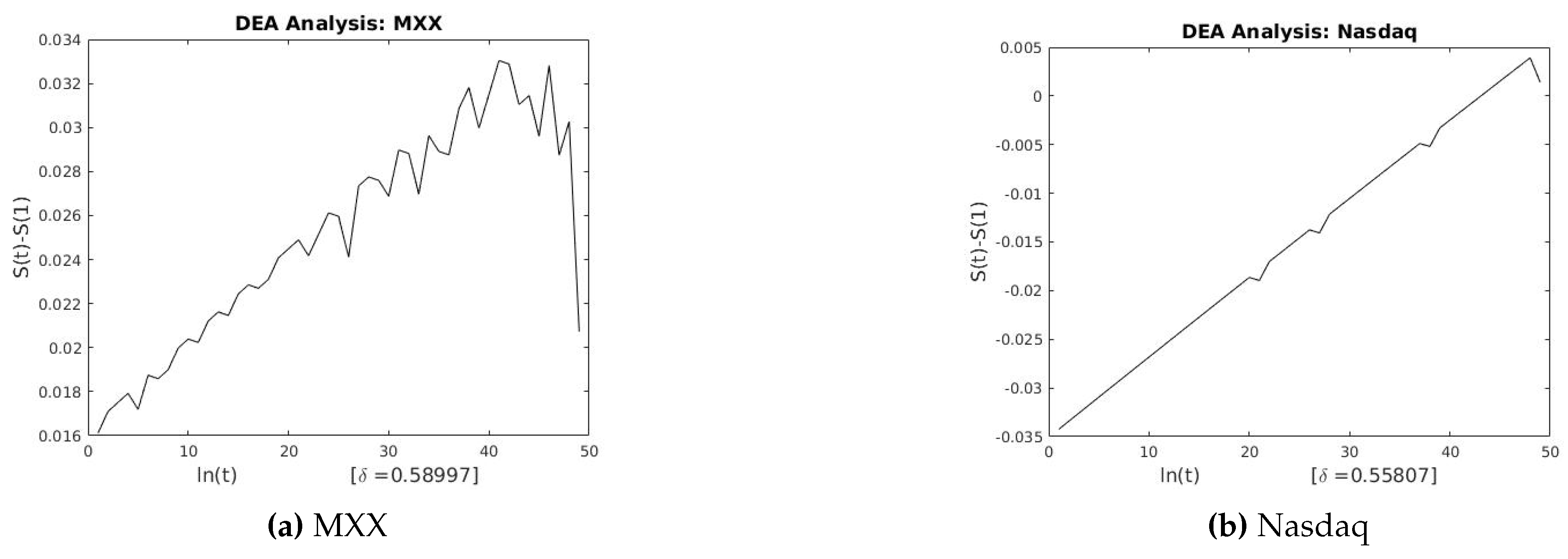
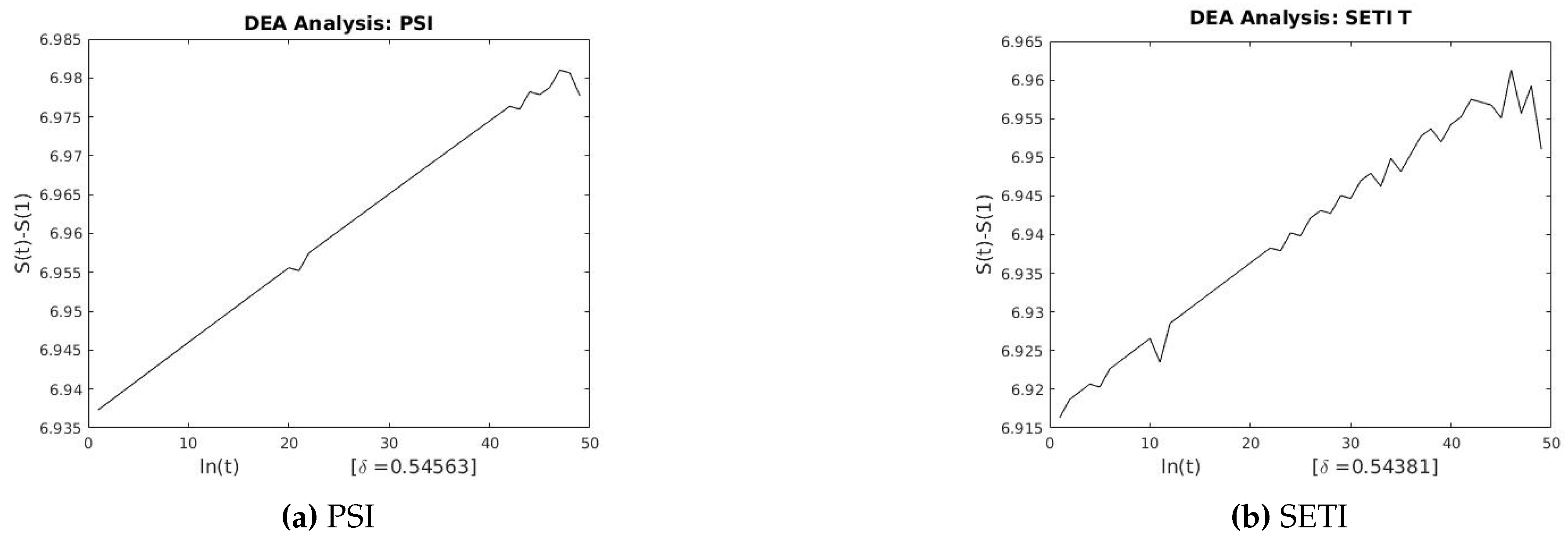
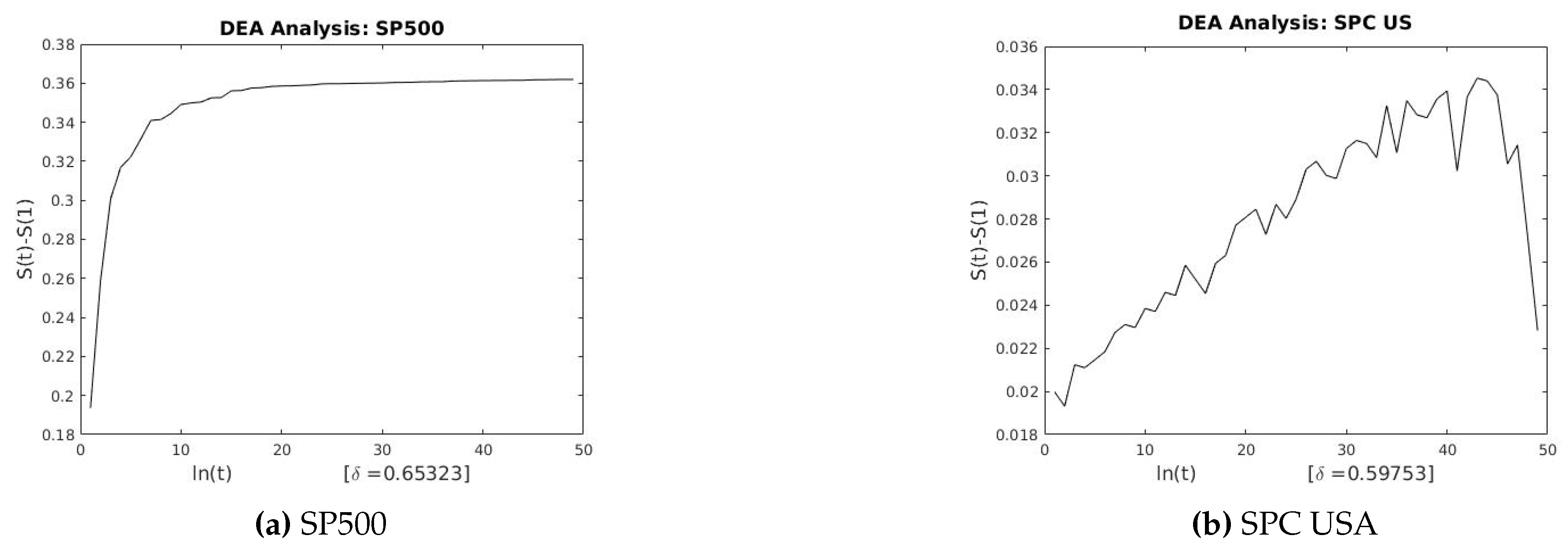
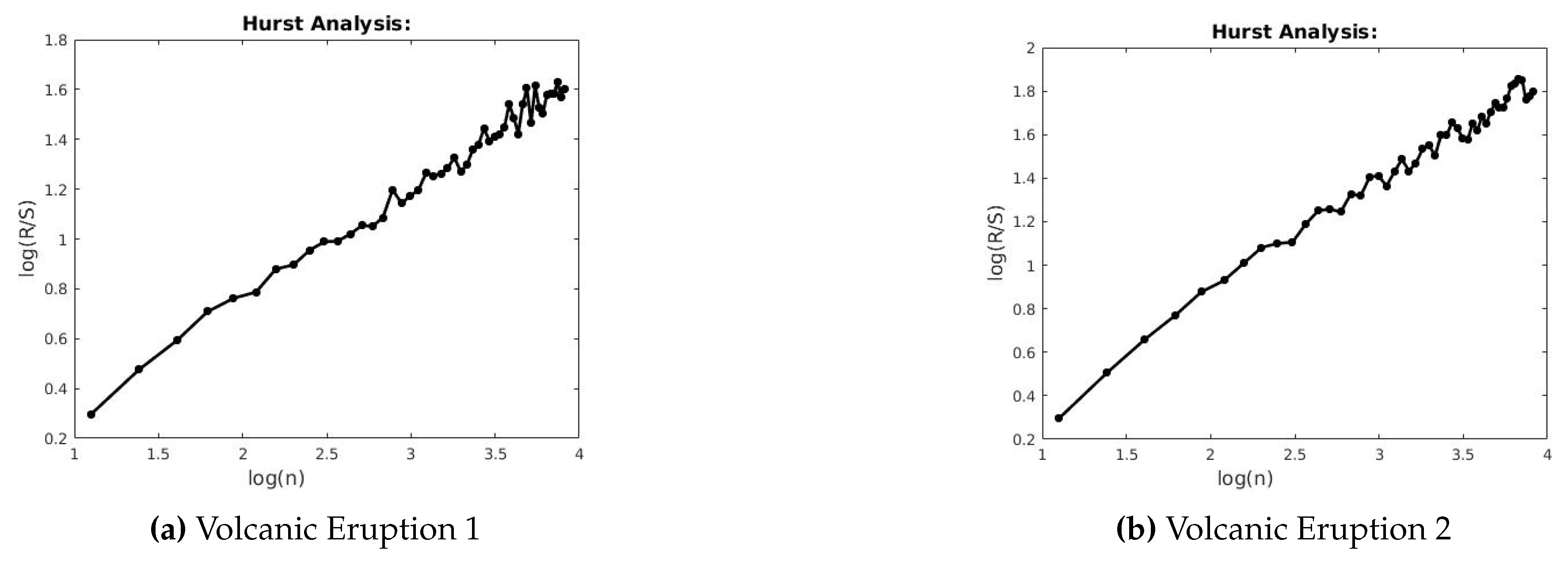
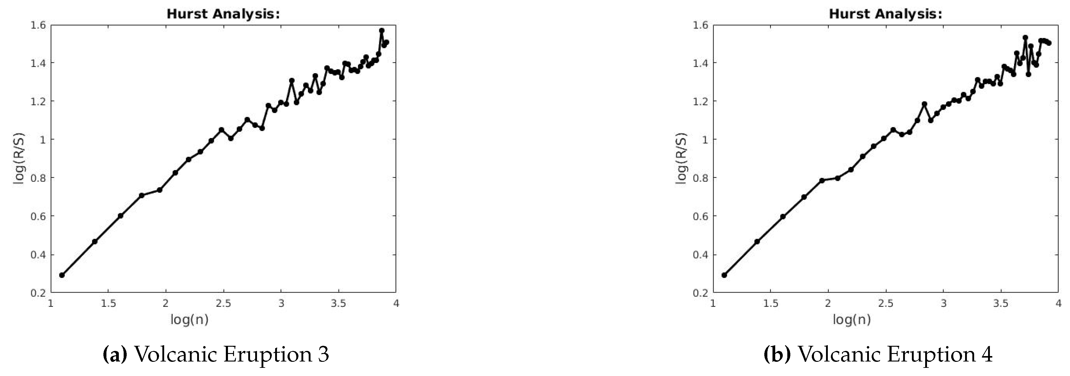
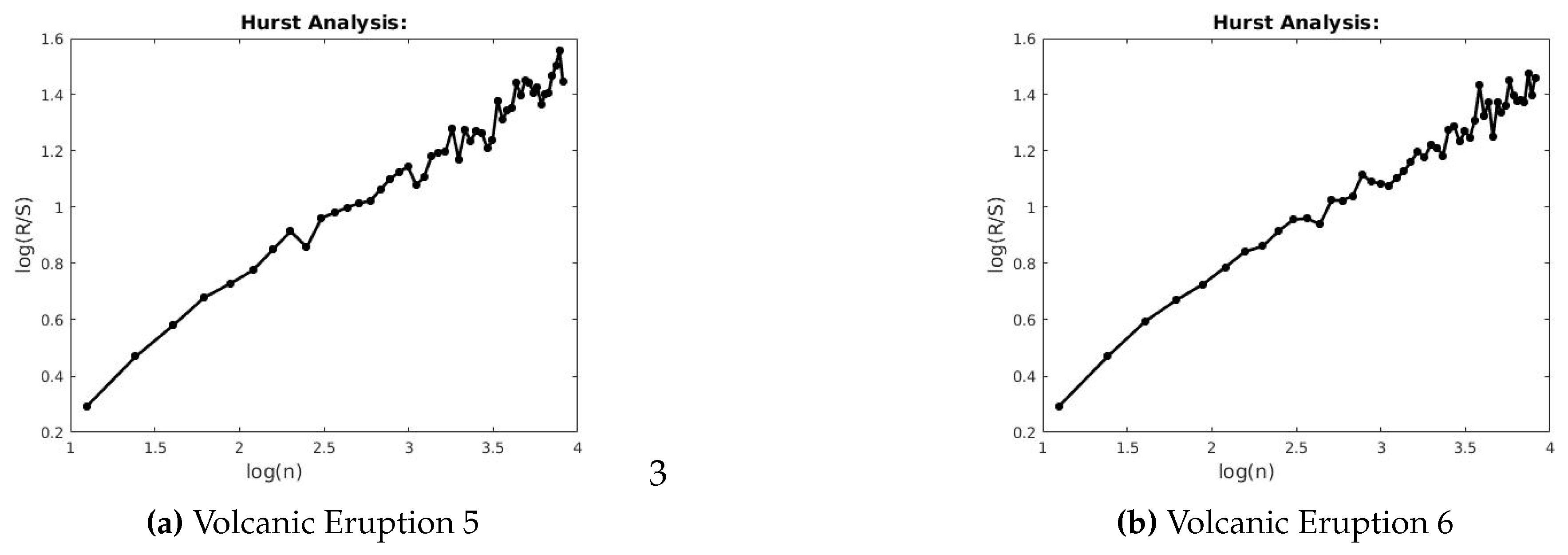
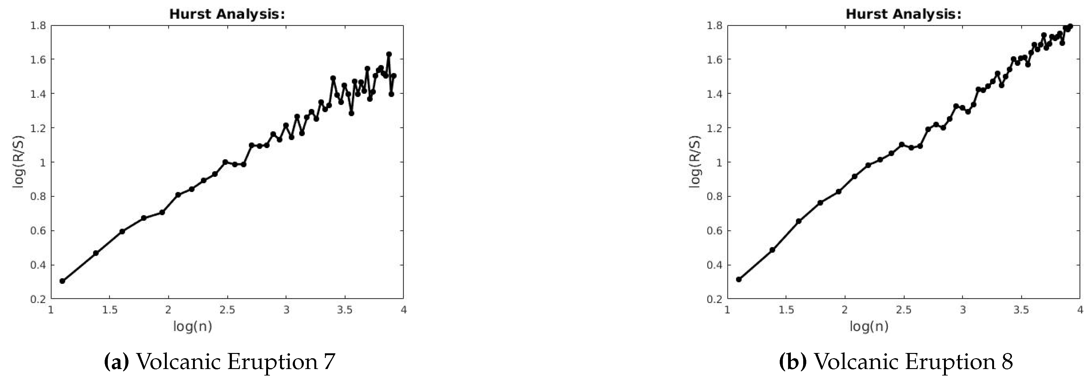
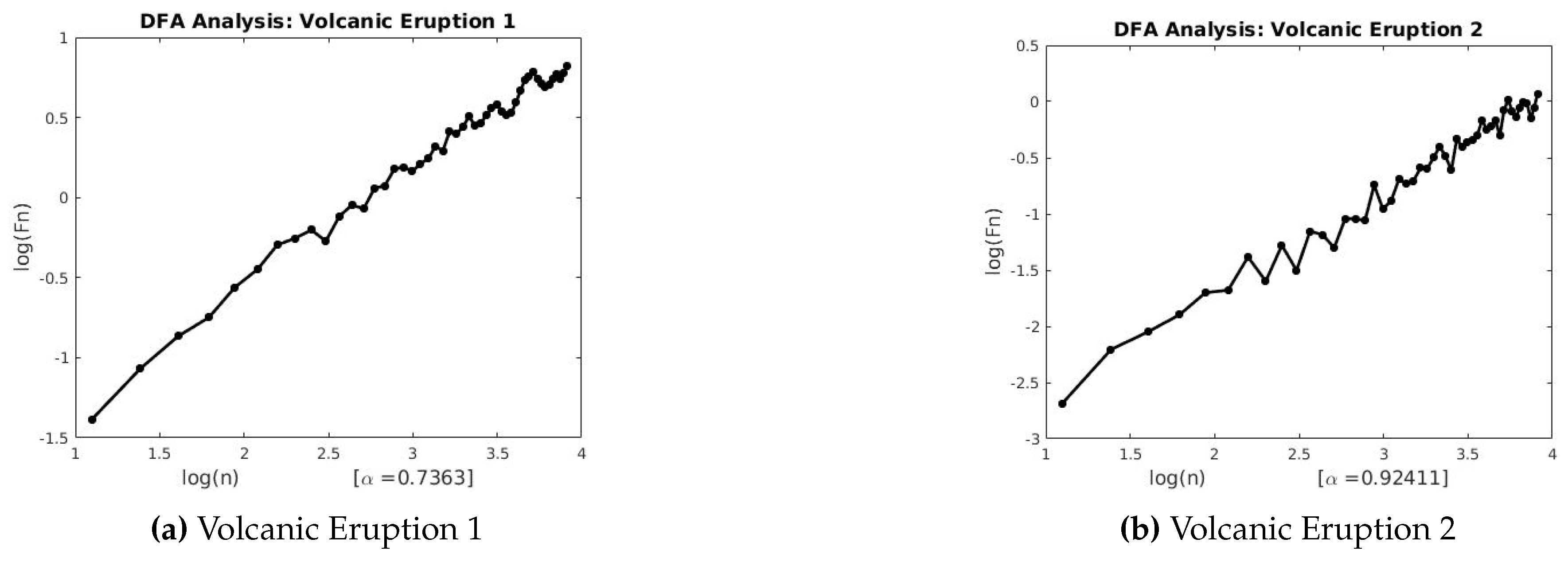
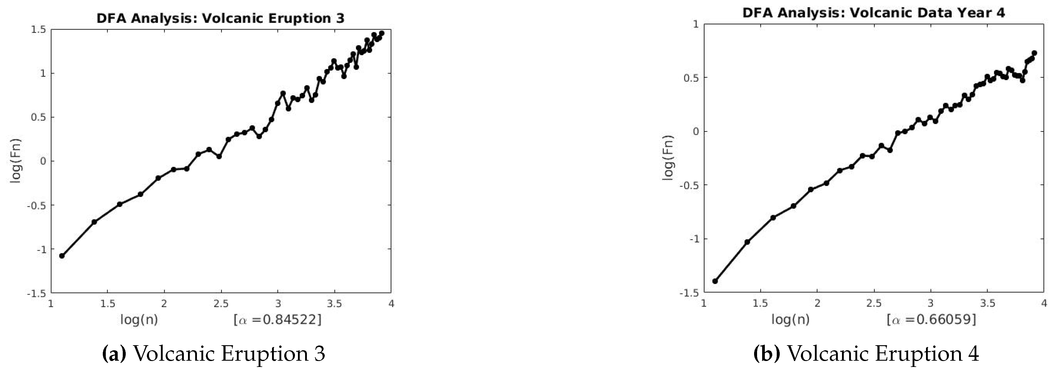
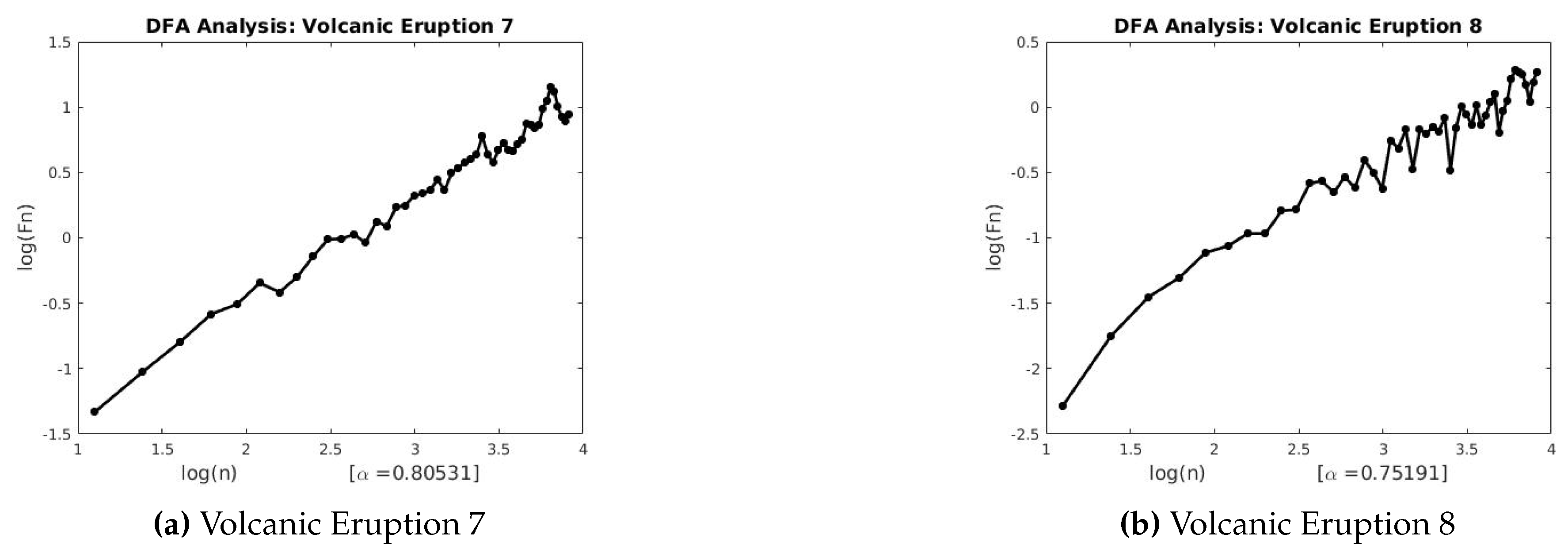
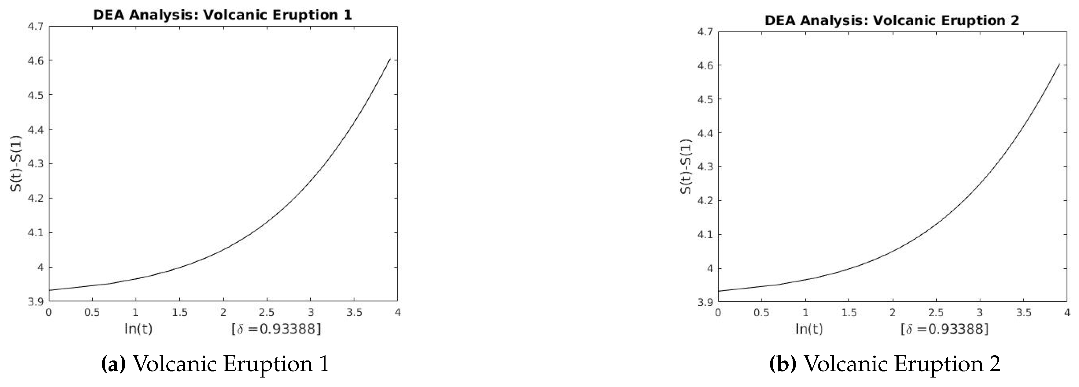
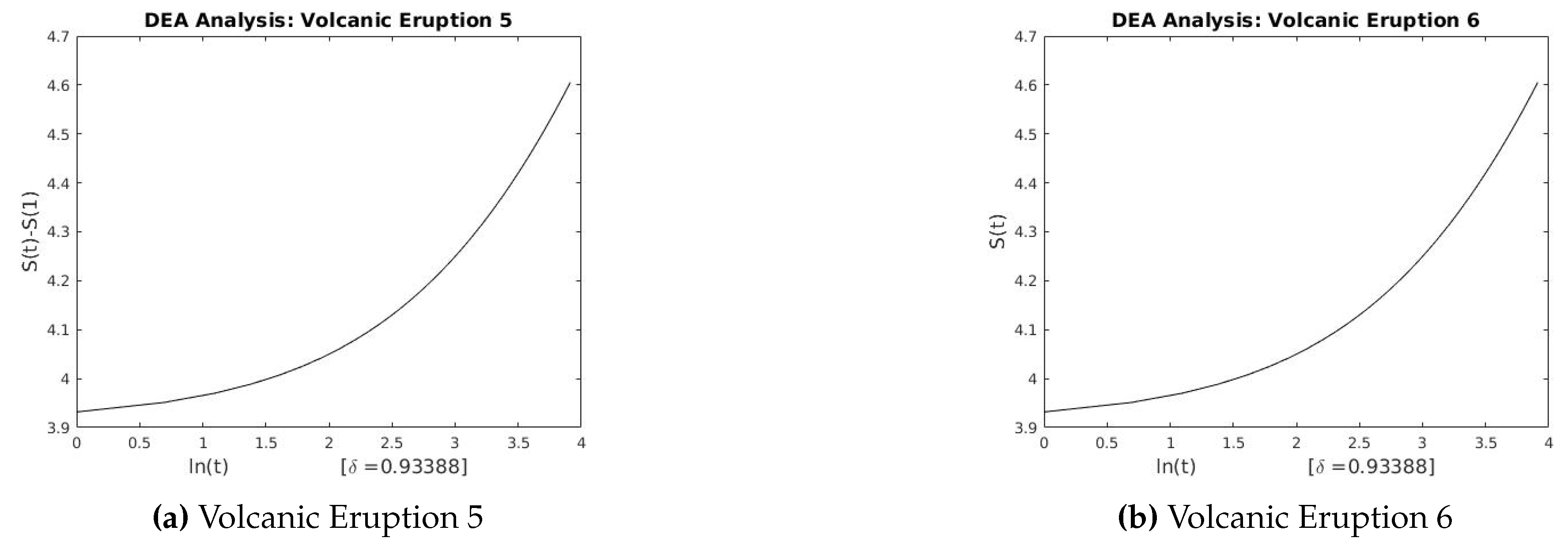
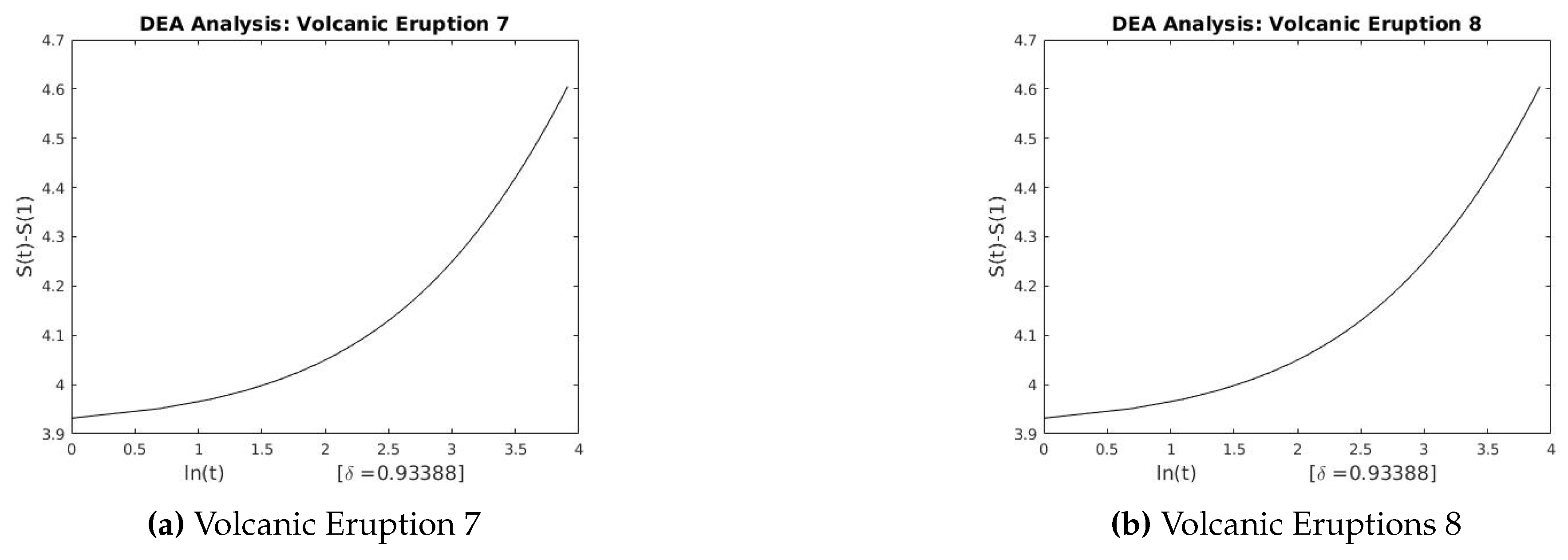
This section describes the analysis of financial indices and volcanic time series when our models are applied to the data sets. Table 3 and Table 4 show the scaling exponents derived from applying the three scaling methods. The δ , H , and α exponents are used to obtain δ L e v y ( R / S ) and δ L e v y ( D F A ) . The Hurst analysis of financial indices and volcano time series are shown in Figures 2–6, 17–20. The slope of the best straight line fitted on the logarithmic plot of rescaled range (R/S) versus time is the Hurst exponent (see Table 3). Figures 7–11 and 21–24 summarize the DFA analysis of financial indices and volcanic eruption, showing the linear trend when plotting ( n ) and F ( n ) on a log-log scale. A linear relationship on a double log graph indicates that there is a scaling or self-similarity in the graph, and the fluctuations can be characterized by scaling exponent. Table 3 and Table 4, Figures 7–11 and 21–24 show that the scaling exponent ( α ) is less than 1, which confirms the presence of long-range correlations, that is, the large values are likely to be followed by large values and vice versa. So the DFA allows us to study the correlations in data, without disturbance of seasonality or trend. In Figures 12–16 and 25–28, we notice that there is a considerable difference between the DEA analysis of financial indices and volcanic eruptions data. Unlike the financial indices, S ( t ) S ( 1 ) of the volcanic eruption data is increased almost exponentially with the logarithm of time scale.

Figures

In this section we present figures obtained from our numerical simulation of the financial and volcanic time series data after we applied the R/S analysis, the DFA and the DEA. Figure 2, Figure 3, Figure 4, Figure 5 and Figure 6 show the log-log plot from the R/S analysis applied on the financial time series. Figure 7, Figure 8, Figure 9, Figure 10 and Figure 11 show the log-log plot of F(n) versus (n), showing the linear trend in the plot. Figure 12, Figure 13, Figure 14, Figure 15 and Figure 16 show the linear-log plot of the financial time series. Figure 17, Figure 18, Figure 19 and Figure 20 show the log-log plot from the R/S analysis applied on the volcanic eruptions. Figure 21, Figure 22, Figure 23 and Figure 24 show the log-log plot of the DFA applied to the volcanic time series. Figure 25, Figure 26, Figure 27 and Figure 28 show the quadratic-log plot of the DEA applied to the volcanic time series.

5. Discussion

For the financial series data all three scaling methods correctly detect the existence of long-range correlations. Comparing δ with the relation in Equation (5), we see that the relation holds (with adjustments within the interval (0, 0.06)) since equality is almost always impossible by virtue of the fact that each scaling method derives its scaling exponent through approximations. Thus we are able to deduce that the financial time series is characterized by a Lévy walk. With the Volcanic data however the R/S analysis is unable to correctly detect the existence of long-range correlations since the volcanic data is non-stationary. However the DEA and DFA correctly detects long-range correlations. Equation (5) is however not satisfied and clearly δ ( H , α ) . Hence the volcanic series can neither be characterized by FBM nor Lévy walk. The volcanic time series is thus characterized by a Lévy flight (i.e., it has an infinite variance).

6. Conclusions

In this study, we have used high frequency financial and volcanic time series to analyze their scaling and dynamic behavior. We have implemented some scaling techniques, namely Diffusion Entropy Analysis, Diffusion Fluctuation Analysis and the R/S analysis that incorporates exponential and Hurst parameters. The techniques allow us to characterize the data distribution and their long-range correlations. To obtain a good fit for the data, we first analyze their stationary behavior using unit root tests (see Section 3.3). Table 3 and Table 4 to confirm that the p-values are significant at all specified levels for financial data, so the high frequency financial indices used in this paper are stationary. In Section 3.3.3, we see that the volcano time series data shows non-stationary behavior. We fit three scaling exponent techniques into our financial and geophysical data in order to estimate the exponent parameters.
Table 3 and Table 4 summarize the estimation of parameters α , δ , and H for financial and volcano data, respectively. We see that the estimated values ( α , δ , and H) fall between 0 and 1, which means that the high frequency stock market data and volcanic eruption data show long memory behavior. The long memory supports that the present information is highly correlated with past information at specified levels, which may facilitate prediction. We conclude that for the high frequency stock market data, the Hurst coefficient is near to 0.65, Detrended fluctuation parameter is near to 0.65, and Diffusion entropy parameter is near to 0.59. For the high frequency volcanic time series, the Hurst coefficient is near to 0.39 and Diffusion entropy parameter is 0.6837. In addition we have shown with a combination of DEA and the variation scaling methods that the financial time series can be characterized by a Lévy walk while the volcanic time series is characterized by a Lévy flight. The Lévy process is useful to detect a financial crash of the stock market or the risky seismic events. Since the high frequency data follow almost log-normal distribution, for any finite-variance Lévy process, randomizing time is equivalent to randomizing variance. Thus the time-varying Lévy process generates stochastic volatility (SV) by randomizing time, which may improve the forecasting performance. The reason is that the SV model takes into account a stochastic component of the data volatility and estimates the time-varying parameters using filtering techniques in order to predict future volatility [30].

Author Contributions

M.C.M. contributed to the supervision and project administration, P.K.A., M.A.M.B., M.P.B.-V., S.J. and O.K.T. contributed to the conceptualization and methodology. All authors have read and approved the final manuscript.

Funding

This research received no external funding.

Conflicts of Interest

The authors declare no conflict of interest.

References

  1. Available online: https://www.physionet.org/tutorials/fmnc/node5.html (accessed on 3 October 2019).
  2. Barany, E.; Beccar Varela, M.P.; Florescu, I.; Sengupta, I. Detecting market crashes by analysing long-memory effects using high-frequency data. Quant. Financ. 2012, 12, 623–634. [Google Scholar] [CrossRef]
  3. Mariani, M.C.; Liu, Y. Normalized truncated Lévy walks applied to the study of financial indices. Physica A 2007, 377, 590–598. [Google Scholar] [CrossRef]
  4. Qi, J.; Yang, H. Hurst exponents for short time series. Phys. Rev. E Stat. Nonlin Soft Matter Phys. 2011, 84, 066114. [Google Scholar] [CrossRef] [PubMed] [Green Version]
  5. Beccar-Varela, M.P.; Gonzales-Huizar, H.; Mariani, M.C.; Tweneboah, O.K. Lévy Flights and Wavelets Analysis of Volcano-Seismic Data. Pure Appl. Geophys. 2019, 177, 723–736. [Google Scholar] [CrossRef]
  6. Lai, G.; Chang, W.C.; Yang, Y.; Liu, H. Modeling long- and short-term temporal patterns with deep neural networks. SIGIR 2018, 95–104. [Google Scholar] [CrossRef] [Green Version]
  7. Scafetta, N. An Entropic Approach to the Analysis of Time Series. Ph.D. Thesis, University of North Texas, Denton, TX, USA, 2001. [Google Scholar]
  8. Scafetta, N.; Grigolini, P. Scaling detection in time series: Diffusion entropy analysis. Phys. Rev. E Stat. Nonliner Soft Matter Phys. 2002, 66, 036130. [Google Scholar] [CrossRef] [Green Version]
  9. Scafetta, N.; Latora, V.; Grigolini, P. Lévy scaling: The diffusion entropy analysis applied to DNA sequences. Phys. Rev. E Stat. Nonliner Soft Matter Phys. 2002, 66, 031906. [Google Scholar] [CrossRef] [Green Version]
  10. Morariu, V.V.; Buimaga-Iarinca, L.; Vamoș, C.; Șoltuz, Ș.M. Detrended fluctuation analysis of autoregressive processes. Fluct. Noise Lett. 2007, 7, L249–L255. [Google Scholar] [CrossRef] [Green Version]
  11. Mariani, M.C.; Tweneboah, O.K. Stochastic differential equations applied to the study of geophysical and financial time series. Physica A 2016, 443, 170–178. [Google Scholar] [CrossRef]
  12. Krištoufek, L. Rescaled range analysis and Detrended Fluctuation Analysis: Finite sample properties and confidence intervals. Czech Econ. Rev. 2010, 4, 315–329. [Google Scholar]
  13. Huang, J.; Shang, P.; Zhao, X. Multifractal diffusion entropy analysis on stock volatility in financial markets. Physica A 2012, 391, 5739–5745. [Google Scholar] [CrossRef]
  14. Haubold, A.; Haubold, H.J.; Kumar, D. Heliosheath: Diffusion Entropy Analysis and Nonextensivity q-triplet. arXiv 2012, arXiv:1202.3417. [Google Scholar]
  15. Brooks, C. A measure of persistence in daily pound exchange rates. Appl. Econ. Lett. 1995, 2, 428–431. [Google Scholar] [CrossRef]
  16. Available online: https://en.wikipedia.org/wiki/Rescaled_range (accessed on 10 October 2019).
  17. Available online: http://fusionwiki.ciemat.es/wiki/Long-range_correlation (accessed on 10 October 2019).
  18. Available online: http://www.ueltschi.org/teaching/chapShannon.pdf (accessed on 15 October 2019).
  19. Hurst, H.E. Long term storage capacity of reservoirs. Trans. Am. Soc. Eng. 1951, 116, 770–799. [Google Scholar]
  20. Timothy, G.; Robert, G.B.; Nicholas, W.; Franzke, C. A brief history of long memory: Hurst, Mandelbrot and the road to ARFIMA. Entropy 2016, 19, 437. [Google Scholar]
  21. Peng, C.K.; Sergey, V.B.; Shlomo, H.; Simons, M.; Stanley, H.E.; Goldberger, A.L. Mosaic organization of DNA nucleotides. Phys. Rev. E Stat. Nonlin. Soft Matter Phys. 1994, 49, 1685. [Google Scholar] [CrossRef] [Green Version]
  22. Buldyrev, S.V.; Goldberger, A.L.; Havlin, S.; Mantegna, R.N.; Matsa, M.E.; Peng, C.K.; Simons, M.; Stanley, H.E. Long-range correlation properties of coding and noncoding DNA sequences: GenBank analysis. Phys. Rev. E Stat. Nonlin. Soft Matter Phys. 1995, 51, 5084. [Google Scholar] [CrossRef]
  23. Heneghan, C.; McDarby, G. Establishing the relation between detrended fluctuation analysis and power spectral density analysis for stochastic processes. Phys. Rev. E Stat. Nonlin. Soft Matter Phys. 2000, 62, 6103. [Google Scholar] [CrossRef] [Green Version]
  24. Siwy, Z.; Ausloos, M.; Ivanova, K. Correlation studies of open and closed state fluctuations in an ion channel: Analysis of ion current through a large-conductance locust potassium channel. Phys. Rev. E Stat. Nonlin. Soft Matter Phys. 2000, 65, 031907. [Google Scholar] [CrossRef] [Green Version]
  25. Janosi, I.M.; Muller, R. Empirical mode decomposition and correlation properties of long daily ozone records. Phys. Rev. E Stat. Nonlin. Soft Matter Phys. 2005, 71, 056126. [Google Scholar] [CrossRef] [Green Version]
  26. Santhanam, M.S.; Bandyopadhyay, J.N.; Angom, D. Quantum spectrum as a time series: Fluctuation measures. Phys. Rev. E Stat. Nonlin. Soft Matter Phys. 2006, 73, 015201. [Google Scholar] [CrossRef] [PubMed] [Green Version]
  27. Talkner, P.; Lutz, E.; Hänggi, P. Fluctuation theorems: Work is not an observable. Phys. Rev. E Stat. Nonlin. Soft Matter Phys. 2007, 75, 032903. [Google Scholar] [CrossRef] [PubMed] [Green Version]
  28. Available online: http://galileo.phys.virginia.edu/classes/152.mf1i.spring02/Entropy.pdf (accessed on 10 October 2019).
  29. Mariani, M.C.; Bhuiyan, M.A.M.; Tweneboah, O.K.; Gonzalez-Huizar, H.; Florescu, I. Volatility models applied to geophysics and high frequency financial market data. Physica A 2018, 503, 304–321. [Google Scholar] [CrossRef] [Green Version]
  30. Mariani, M.C.; Bhuiyan, M.A.M.; Tweneboah, O.K. Estimation of stochastic volatility by using Ornstein–Uhlenbeck type models. Physica A 2018, 491, 167–176. [Google Scholar] [CrossRef]
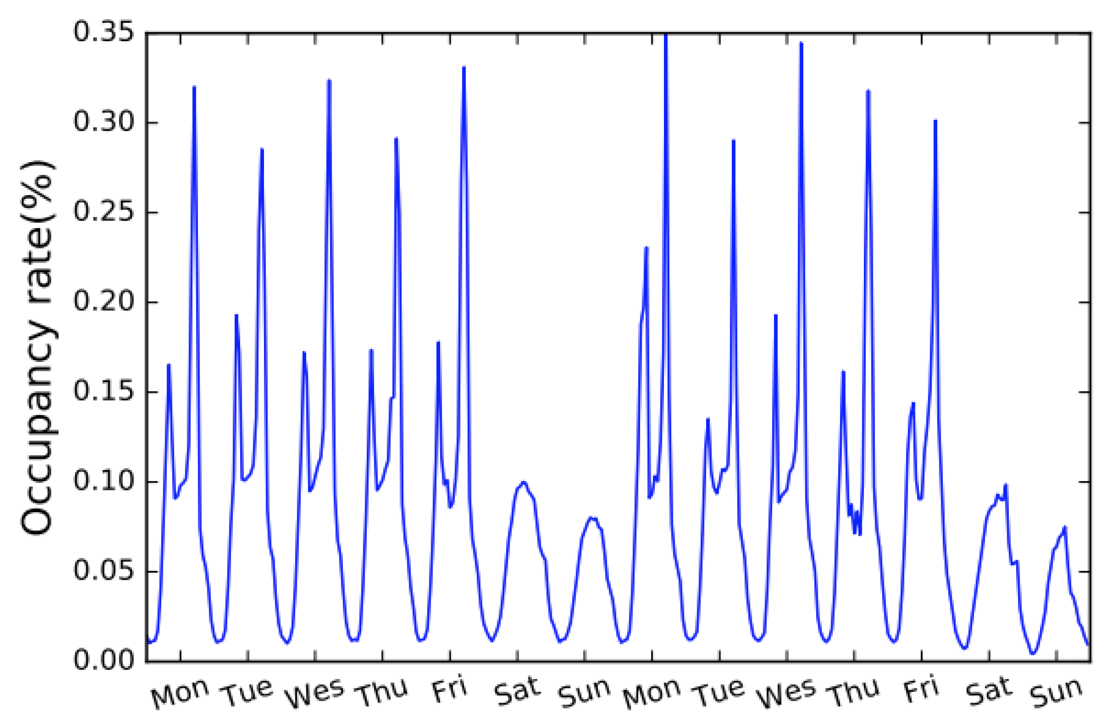
Figure 1. The hourly occupancy rate of a road in the bay area for 2 weeks [6].
Mathematics 08 00441 g001
Figure 2. R/S analysis for BVSP and HSI.
Mathematics 08 00441 g002
Figure 3. R/S analysis for IGPA and MERV.
Mathematics 08 00441 g003
Figure 4. R/S analysis for MXX and Nasdaq.
Mathematics 08 00441 g004
Figure 5. R/S analysis for PSI and SETI.
Mathematics 08 00441 g005
Figure 6. R/S analysis for SP500 and SPC USA.
Mathematics 08 00441 g006
Figure 7. Detrended Fluctuation Analysis (DFA) for BVSP and HSI.
Mathematics 08 00441 g007
Figure 8. DFA for IGPA and MERV.
Mathematics 08 00441 g008
Figure 9. DFA for MXX and Nasdaq.
Mathematics 08 00441 g009
Figure 10. DFA for PSI and SETI.
Mathematics 08 00441 g010
Figure 11. DFA for SP500 and SPC USA.
Mathematics 08 00441 g011
Figure 12. DEA for BVSP and HSI.
Mathematics 08 00441 g012
Figure 13. DEA for IGPA and MERV.
Mathematics 08 00441 g013
Figure 14. DEA for MXX and Nasdaq.
Mathematics 08 00441 g014
Figure 15. DEA for PSI and SETI.
Mathematics 08 00441 g015
Figure 16. DEA for SP500 and SPC USA.
Mathematics 08 00441 g016
Figure 17. R/S for Volcanic Eruptions 1 and 2.
Mathematics 08 00441 g017
Figure 18. R/S for Volcanic Eruptions 3 and 4.
Mathematics 08 00441 g018
Figure 19. R/S for Volcanic Eruptions 5 and 6.
Mathematics 08 00441 g019
Figure 20. R/S for Volcanic Eruptions 7 and 8.
Mathematics 08 00441 g020
Figure 21. DFA for Volcanic Eruptions 1 and 2.
Mathematics 08 00441 g021
Figure 22. DFA for Volcanic Eruptions 3 and 4.
Mathematics 08 00441 g022
Figure 23. DFA for Volcanic Eruptions 5 and 6.
Mathematics 08 00441 g023
Figure 24. DFA for Volcanic Eruptions 7 and 8.
Mathematics 08 00441 g024
Figure 25. DEA for Volcanic Eruptions 1 and 2.
Mathematics 08 00441 g025
Figure 26. DEA for Volcanic Eruptions 3 and 4.
Mathematics 08 00441 g026
Figure 27. DEA for Volcanic Eruptions 5 and 6.
Mathematics 08 00441 g027
Figure 28. DEA for Volcanic Eruptions 7 and 8.
Mathematics 08 00441 g028
Table 1. Augmented Dickey-Fuller test (ADF) test applied to the financial time series: p-values.
Marketp-Value
BVSP0.015
SPC0.034
HSI0.033
IGPA0.03
MERV0.014
MXX0.024
Nasdaq0.04
PSI<0.01
SETI<0.01
SP500<0.01
XU1000.01
Table 2. ADF test applied to the Volcanic time series: p-values.
Eruption Numberp-Value
10.3568
20.6747
30.3024
40.095
50.2064
60.3271
70.2374
80.4059
Table 3. Scaling exponents for emerging and established markets time series.
MarketR/S(H)DFA ( α )DEA ( δ ) δ Levy (R/S) δ Levy (DFA)
BVSP0.590.720.570.560.63
SPC0.590.620.600.560.56
HSI0.650.70.600.560.63
IGPA0.740.650.530.630.56
MERV0.620.620.560.560.56
MXX0.640.660.590.560.56
Nasdaq0.60.720.560.560.56
PSI0.660.710.550.630.56
SETI0.640.700.540.560.56
SP5000.630.660.650.580.60
XU1000.640.700.540.560.56
Table 4. Scaling exponents of Volcanic Data time series.
Eruption NumberR/S(H)DFA ( α )DEA ( δ ) δ Levy (R/S) δ Levy (DFA)
10.450.740.68370.47560.6547
20.510.920.68370.50930.8682
30.380.850.68370.44720.7636
40.390.660.68370.45090.5957
50.390.760.68370.45130.6729
60.370.670.68370.44330.6002
70.420.810.68370.46340.7194
80.5040.750.68370.50180.6684