A Fast Image Restoration Algorithm Based on a Fixed Point and Optimization Method

Abstract

In this paper, a new accelerated fixed point algorithm for solving a common fixed point of a family of nonexpansive operators is introduced and studied, and then a weak convergence result and the convergence behavior of the proposed method is proven and discussed. Using our main result, we obtain a new accelerated image restoration algorithm, called the forward-backward modified W-algorithm (FBMWA), for solving a minimization problem in the form of the sum of two proper lower semi-continuous and convex functions. As applications, we apply the FBMWA algorithm to solving image restoration problems. We analyze and compare convergence behavior of our method with the others for deblurring the image. We found that our algorithm has a higher efficiency than the others in the literature.

1. Introduction

It is well-known that fixed point theory has relevant applications in many branches of analysis [1,2,3,4,5,6,7,8,9] and it can be applied to solving many areas of science and applied science, engineering, economics and medicine, such as image/signal processing [10,11,12,13,14,15,16,17] and modeling intensity modulated radiation theory treatment planning [18,19,20]. Many real life problems can be equivalently formulated as fixed point problems, meaning that one has to find a fixed point of some operators. One of most popular fixed point algorithms is Picard iteration. Up to now, many fixed point algorithms have been introduced and studied to solve various kinds of real world problems, such as Mann iteration [7], Ishikawa iteration [4], SP-iteration [21] and W-iteration [22].

The image restoration problem is an important topic in image processing. This problem can be transformed to an optimization problem using the least absolute shrinkage and selection operator (LASSO) model. There are several optimization and fixed point methods for such problem; see [23,24,25,26,27] for examples. One of the most popular methods for solving the image restoration problem is FISTA (fast iterative shrinkage-thresholding algorithm). This method was shown by Beck and Teboulle in [28] to have more efficiency than the previous methods in the literature.

In this paper, we focus our attention on a new accelerated algorithm that has been developed from the view of fixed point. For instance, Wongyai and Suantai [22] proposed the W-algorithm for solving a fixed point problem of a continuous function, and proved that the W-algorithm has a convergence rate better than the others. Motivated by this idea, we propose a new algorithm by modification of W-algorithm for solving a common fixed point problem of a countable family of nonexpansive operators. We also prove the convergence of our algorithm under some conditions and apply it to solving the image restoration problem and compare its efficiency with other methods in term of PSNR (peak signal-to-noise ratio).

The organization of this paper is as follows. In Section 2, we briefly describe background and related algorithms in the literature. In Section 3, we describe some notation and useful lemmas for the latter section. In Section 4, we introduce our proposed algorithm for the common fixed point problem, giving the theoretical proofs of its convergence under particular conditions. In Section 5, we apply our algorithm to solving the image restoration problem and compare its performance with other existing methods. Finally, we conclude our work in Section 6.

2. Background and Related Algorithms

In this section, we recall the background of a mathematical model for the image restoration problem and some related algorithms used to solving this problem. A simple model for image restoration problem is formulated by the linear model:

$$Ay=a+v,$$

(1)

where $y\in {\mathbb{R}}^{n\times 1}$ is an original image, $a\in {\mathbb{R}}^{m\times 1}$ is the observed image, v is additive noise and $A\in {\mathbb{R}}^{m\times n}$ is the blurring operation. In order to solve the problem (1), Tibshirani in [29], introduced the least absolute shrinkage and selection operator (LASSO) for solving the following minimization problem:

$$\underset{y}{min}\{{\parallel Ay-a\parallel }_2^2+\lambda {\parallel y\parallel }_1\},$$

(2)

where $\lambda >0$ is a regularization parameter, ${\parallel y\parallel }_1={\sum }_{i=1}^n\left|y_i\right|,$ and ${\parallel y\parallel }_2=\sqrt{{\sum }_{i=1}^n{\left|y_i\right|}^2}.$ The general minimization problem which includes (2) as a special case is the following minimization problem:

$$\underset{y\in {\mathbb{R}}^n}{min}\{F\left(y\right):=f\left(y\right)+h\left(y\right)\},$$

(3)

where $h:{\mathbb{R}}^n\to \mathbb{R}\cup \{+\infty \}$ is proper convex and lower semi-continuous, and $f:{\mathbb{R}}^n\to \mathbb{R}$ is a convex and differentiable function such that $\nabla f$ is a Lipschitz continuity with constant $L>0.$ The set of minimizers of F is denoted by $Argmin\left(F\right).$

The classical forward-backward splitting (FBS) algorithm [30] for problem (3) is given by the following iterative formula:

$$x_{n+1}=\underset{\mathrm{backward}\mathrm{step}}{\underbrace{pro{x}_{c_{n}h}}} \underset{\mathrm{forward}\mathrm{step}}{\underbrace{(I-c_n\nabla f)}}\left(x_n\right),c_n\in (0,2/L),n\in \mathbb{N},$$

(4)

where $x_1\in {\mathbb{R}}^n,$$c_n$ is the step-size, I is an identity operator and $pro{x}_h$ is the proximity operator of h defined by $pro{x}_h\left(x\right):=\underset{y}{argmin}\{h\left(y\right)+\frac{1}{2}{\parallel x-y\parallel }_2^2\}$; see [31] for more details. In different literature, FBS is also called the iterative denoising method [32], Landweber iteration [33] or the fixed point continuation (FPC) algorithm [34]. In the last several years, some acceleration techniques have been proposed in order to accelerate the convergence rate of the studied algorithms.

The inertial forward-backward splitting (IFBS) was proposed by Moudafi and Oliny in [35] as follows:

$$\begin{array}{c}{y}_n=x_n+{\theta }_n(x_n-x_{n-1}),\hfill \\ x_{n+1}=pro{x}_{c_{n}h}(y_n-c_n\nabla f\left(x_n\right)),c_n\in (0,2/L),n\in \mathbb{N},\hfill \end{array}$$

(5)

where $x_0,x_1\in {\mathbb{R}}^n,$${\theta }_n$ is the inertial parameter which controls the momentum $x_n-x_{n-1}.$ The convergence of IFBS can be guaranteed under proper choices of $c_n$ and ${\theta }_n.$

The fast iterative shrinkage-thresholding algorithm (FISTA) was proposed by Beck and Teboulle in [28] as follows:

$$\{\begin{array}{c}{y}_n=pro{x}_{\frac{1}{L}h}(x_n-\frac{1}{L}\nabla f(x_n)),\hfill \\ t_{n+1}=\frac{1+\sqrt{1+4t_n^2}}{2},{\theta }_n=\frac{t_n-1}{t_{n+1}},\hfill \\ x_{n+1}=y_n+{\theta }_n(y_n-y_{n-1}),n\in \mathbb{N},\hfill \end{array}$$

(6)

where $x_1=y_0\in {\mathbb{R}}^n,t_1=1.$ They proved the convergence rate of the FISTA and applied the FISTA to image restoration problem. Very recently, Liang and Schonlieb [36] modified FISTA by replacing $t_{n+1}=(p+\sqrt{q+r{t}_n^2})/2$ where $p,q>0$ and $0<r\le 4,$ and proved the weak convergence theorem of FISTA.

The new accelerated proximal gradient algorithm (NAGA) was proposed by Verma and Shukla in [37] as follows:

$$\begin{array}{c}{y}_n=x_n+{\theta }_n(x_n-x_{n-1}),\hfill \\ x_{n+1}=T_n[(1-{\alpha }_n)y_n+{\alpha }_n{T}_n{y}_n],n\in \mathbb{N},\hfill \end{array}$$

(7)

where $x_0,x_1\in {\mathbb{R}}^n,$$T_n$ is the forward-backward operator of f and h with respect to $c_n\in (0,2/L).$ They proved the convergence and stability of the algorithm under a few specific conditions, and applied the algorithm for solving the convex minimization problem with sparsity-inducing regularizes for multitask learning framework.

3. Preliminaries

Let us review some important definitions and useful lemmas needed for the convergence theorem presented in the next section.

Let H be a real Hilbert space with norm $\parallel ·\parallel$ and inner product $\langle ·,·\rangle ,$ and C be a nonempty closed convex subset of $H.$ A mapping $T:C\to C$ is said to be a L-Lipschitz operator if there exists $L>0$ such that $\parallel Tx-Ty\parallel \le L\parallel x-y\parallel$ for all $x,y\in C.$ An L-Lipschitz operator is called a nonexpansive operator if $L=1.$ The set of all fixed points of T is denoted by $Fix\left(T\right)$; i.e., $Fix\left(T\right):=\{x\in C:Tx=x\}.$ Let $\left\{T_n\right\}$ and $\mathsf{\Omega }$ be families of nonexpansive operators of C into itself such that $\varnothing \ne Fix\left(\mathsf{\Omega }\right)\subset \mathsf{\Gamma }:={\cap }_{n=1}^{\infty }Fix\left(T_n\right),$ where $Fix\left(\mathsf{\Omega }\right)$ is the set of all common fixed points of $\mathsf{\Omega },$ and let ${\omega }_w\left(x_n\right)$ denote the set of all weak-cluster points of a bounded sequence $\left\{x_n\right\}$ in $C.$ A sequence $\left\{T_n\right\}$ is said to satisfy the NST (Nakajo, Shimoji and Takahashi1)-condition (I) with $\mathsf{\Omega }$ [38], if for every bounded sequence $\left\{x_n\right\}$ in $C,$

$$\underset{n\to +\infty }{lim}\parallel x_n-T_n{x}_n\parallel =0⟹\underset{n\to +\infty }{lim}\parallel x_n-T{x}_n\parallel =0\forall T\in \mathsf{\Omega }.$$

(8)

If $\mathsf{\Omega }$ is singleton, i.e., $\mathsf{\Omega }=T,$ then $\left\{T_n\right\}$ is said to satisfy the NST-condition (I) with $T.$ After that, Nakajo et al. [39] introduced the NST* condition which is more general than that of NST-condition. A sequence $\left\{T_n\right\}$ is said to satisfy the NST*-condition if for every bounded sequence $\left\{x_n\right\}$ in $C,$

$$\underset{n\to +\infty }{lim}\parallel x_n-T_n{x}_n\parallel =\underset{n\to +\infty }{lim}\parallel x_n-x_{n+1}\parallel =0⟹{\omega }_w\left(x_n\right)\subset \mathsf{\Gamma }.$$

(9)

It follows directly from above definition that if $\left\{T_n\right\}$ satisfies the NST-condition (I), then $\left\{T_n\right\}$ satisfies the NST*-condition. Observe that if $h:H\to \mathbb{R}\cup \{+\infty \}$ is a proper, convex and lower semicontinuous function, then for all $x\in H$ the $pro{x}_h\left(x\right)$ exists and is unique; cf. [40]. It is well-known that

$$x^{*}\in Argmin(f+h)⟺0\in \partial h\left(x^{*}\right)+\nabla f\left(x^{*}\right),$$

where $\partial h$ is the subdifferential of h defined by $\partial h\left(x^{*}\right):=\{u:h\left(x\right)\ge \langle u,x-x^{*}\rangle +h\left(x^{*}\right)\forall x\}$ and $\nabla f$ is the gradient of f; see [41] for more details.

Note that the subdifferential operator $\partial h$ is a maximal monotone (see [42] for more details) and the solution of (3) is a fixed point of the following operator:

$$\begin{array}{c}\hfill x^{*}\in Argmin(f+h)⟺x^{*}=J_{c\partial h}(I-c\nabla f)\left(x^{*}\right)=pro{x}_{ch}(I-c\nabla f)\left(x^{*}\right),\end{array}$$

where $c>0$ and $J_{\partial h}$ is the resolvent of $\partial h$ defined by $J_{\partial h}={(I+\partial h)}^{-1}.$ If $c\in (0,\frac{2}{L}),$ we know that $pro{x}_{ch}(I-c\nabla f)$ is a nonexpansive mapping. The operator $pro{x}_{ch}(I-c\nabla f)$ is known as the forward-backward operator of f and h with respect to $c.$ We end this part with the following lemmas which will be used to prove our main results.

Lemma 1.

([43]). For a real Hilbert space $H,$ let $h:H\to \mathbb{R}\cup \{+\infty \}$ be proper convex and lower semi-continuous function, and $f:H\to \mathbb{R}$ be convex differentiable with gradient $\nabla f$ being L-Lipschitz constant for some $L>0.$ If $\left\{T_n\right\}$ is the forward-backward operator of f and h with respect to $c_n\in (0,2/L)$ such that $c_n$ converges to $c,$ then $\left\{T_n\right\}$ satisfies NST-condition (I) with $T,$ where T is the forward-backward operator of f and h with respect to $c\in (0,2/L).$

Lemma 2.

([44]). Let H be a real Hilbert space. Then the following results hold:

(i) 

${\parallel tu+(1-t)v\parallel }^2={t\parallel u\parallel }^2+{(1-t)\parallel v\parallel }^2-t(1-t){\parallel u-v\parallel }^2$$\forall t\in [0,1],$$\forall u,v\in H;$

(ii) 

${\parallel u\pm v\parallel }^2={\parallel u\parallel }^2\pm 2\langle u,v\rangle +{\parallel v\parallel }^2$$\forall u,v\in H.$

Lemma 3.

([45]). Let $\left\{a_n\right\},\left\{b_n\right\}$ and $\left\{{\gamma }_n\right\}$ be sequences of nonnegative real numbers such that $a_{n+1}\le (1+{\gamma }_n)a_n+b_n,n\in \mathbb{N}.$ If ${\sum }_{n=1}^{\infty }{\gamma }_n<+\infty$ and ${\sum }_{n=1}^{\infty }{b}_n<+\infty ,$ then ${lim}_{n\to +\infty }{a}_n$ exists.

Lemma 4.

(Opial [46]). Let H be a Hilbert space and $\left\{x_n\right\}$ be a sequence in H such that there exists a nonempty set $\mathsf{\Gamma }\subset H$ satisfying

(i) 

For every$p\in \mathsf{\Gamma },$${lim}_{n\to +\infty }\parallel x_n-p\parallel$exists;

(ii) 

Each weak-cluster point of the sequence$\left\{x_n\right\}$is in$\mathsf{\Gamma }.$

Then there exists$x^{*}\in \mathsf{\Gamma }$such that$\left\{x_n\right\}$weakly converges to$x^{*}.$

4. Main Results

In this section, we propose a modified W-algorithm which is called “MWA” for finding a common fixed point of a countable family of nonexpansive operators in a real Hilbert space. We are now ready to introduce the MWA algorithm by assuming the following:

• H is a real Hilbert space;
• $\{T_n:H\to H\}$ is a family of nonexpansive operators;
• $\left\{T_n\right\}$ satisfies the NST*-condition;
• $\mathsf{\Gamma }:={\cap }_{n=1}^{\infty }Fix\left(T_n\right)\ne \varnothing .$

We aim to prove a weak convergence theorem of Algorithm 1 (MWA) to a common fixed point of $T_n.$ We start with the following supporting lemma.

Lemma 5.

Let$\left\{a_n\right\}$and$\left\{{\theta }_n\right\}$be sequences of nonnegative real numbers such that

$$a_{n+1}\le (1+{\theta }_n)a_n+{\theta }_n{a}_{n-1},n\in \mathbb{N}.$$

Then the following holds

$$a_{n+1}\le K·\prod _{j=1}^n(1+2{\theta }_j),\mathit{where}K=max\{a_1,a_2\}.$$

Moreover, if${\sum }_{n=1}^{\infty }{\theta }_n<+\infty ,$then$\left\{a_n\right\}$is bounded.

Proof. 

Given $K=max\{a_1,a_2\},$ we have

$$\begin{array}{cc}\hfill a_3& \le (1+2{\theta }_2)K,\hfill \\ \hfill a_4& \le (1+{\theta }_3)a_3+{\theta }_3{a}_2\le (1+{\theta }_3)(1+2{\theta }_2)K+{\theta }_{3}K\hfill \\ \hfill & \le (1+{\theta }_3)(1+2{\theta }_2)K+{\theta }_3(1+2{\theta }_2)K=(1+2{\theta }_3)(1+2{\theta }_2)K.\hfill \end{array}$$

By Mathematical induction, we obtain

$$\begin{array}{c}\hfill a_{n+1}\le K·\prod _{j=2}^n(1+2{\theta }_j)\le K·\prod _{j=1}^n(1+2{\theta }_j).\end{array}$$

Note that the infinite product of the $(1+2{\theta }_j)$ converges if the infinite sum of the ${\theta }_j$ converges. Indeed, $\left\{a_n\right\}$ is bounded if ${\sum }_{n=1}^{\infty }{\theta }_n<+\infty .$ ☐

Algorithm 1: (MWA): A modified W-algorithm

Initial. Take $x_0,x_1\in H$ arbitrarily and $n=1.$ Step 1. Compute $w_n,z_n,y_n$ and $x_{n+1}$ using $$\{\begin{array}{c}{w}_n=x_n+{\theta }_n(x_n-x_{n-1}),\hfill \\ z_n=(1-{\gamma }_n)w_n+{\gamma }_n{T}_n{w}_n,\hfill \\ y_n=(1-{\beta }_n)T_n{w}_n+{\beta }_n{T}_n{z}_n,\hfill \\ x_{n+1}=(1-{\alpha }_n)T_n{z}_n+{\alpha }_n{T}_n{y}_n,\hfill \end{array}$$ Then update $n:=n+1$ and go to Step 1.

Now, we present the main convergence result of Algorithm 1 (MWA) under some suitable control conditions.

Theorem 6.

Let$\left\{x_n\right\}$be a sequence generated by Algorithm 1 (MWA) where${\gamma }_n\in [a_1,b_1]\subset (0,1),{\beta }_n\in [0,1],{\alpha }_n\in [0,b_2]\subset [0,1),{\theta }_n\ge 0$and${\sum }_{n=1}^{\infty }{\theta }_n<+\infty .$Then the following hold:

(i) 

$\parallel x_{n+1}-x^{*}\parallel \le K·{\prod }_{j=1}^n(1+2{\theta }_j),$where$K=max\{\parallel x_1-x^{*}\parallel ,\parallel x_2-x^{*}\parallel \}$and$x^{*}\in \mathsf{\Gamma }.$

(ii) 

$\left\{x_n\right\}$converges weakly to a point in$\mathsf{\Gamma }.$

Proof. 

(i) Let $x^{*}\in \mathsf{\Gamma }.$ By Algorithm 1, we have

$$\begin{array}{cc}\hfill \parallel w_n-x^{*}\parallel & \le \parallel x_n-x^{*}\parallel +{\theta }_n\parallel x_n-x_{n-1}\parallel ,\hfill \end{array}$$

(10)

$$\begin{array}{cc}\hfill \parallel z_n-x^{*}\parallel & \le (1-{\gamma }_n)\parallel w_n-x^{*}\parallel +{\gamma }_n\parallel T_n{w}_n-x^{*}\parallel \le \parallel w_n-x^{*}\parallel ,\hfill \end{array}$$

(11)

$$\begin{array}{cc}\hfill \parallel y_n-x^{*}\parallel & \le (1-{\beta }_n)\parallel T_n{w}_n-x^{*}\parallel +{\beta }_n\parallel T_n{z}_n-x^{*}\parallel \hfill \\ \hfill & \le (1-{\beta }_n)\parallel w_n-x^{*}\parallel +{\beta }_n\parallel z_n-x^{*}\parallel \hfill \\ \hfill & \le \parallel w_n-x^{*}\parallel ,\hfill \end{array}$$

(12)

and

$$\begin{array}{cc}\hfill \parallel x_{n+1}-x^{*}\parallel & \le (1-{\alpha }_n)\parallel T_n{z}_n-x^{*}\parallel +{\alpha }_n\parallel T_n{y}_n-x^{*}\parallel \hfill \\ \hfill & \le (1-{\alpha }_n)\parallel z_n-x^{*}\parallel +{\alpha }_n\parallel y_n-x^{*}\parallel \hfill \\ \hfill & \le \parallel w_n-x^{*}\parallel .\hfill \end{array}$$

(13)

From (10) and (13), we get

$$\parallel x_{n+1}-x^{*}\parallel \le \parallel x_n-x^{*}\parallel +{\theta }_n\parallel x_n-x_{n-1}\parallel .$$

(14)

This implies

$$\begin{array}{c}\hfill \parallel x_{n+1}-x^{*}\parallel \le (1+{\theta }_n)\parallel x_n-x^{*}\parallel +{\theta }_n\parallel x_{n-1}-x^{*}\parallel .\end{array}$$

(15)

Apply Lemma 5, we get $\parallel x_{n+1}-x^{*}\parallel \le K·{\prod }_{j=1}^n(1+2{\theta }_j),$ where $K=max\{\parallel x_1-x^{*}\parallel ,\parallel x_2-x^{*}\parallel \}.$ Since ${\sum }_{n=1}^{\infty }{\theta }_n<+\infty ,$ it follows that $\left\{x_n\right\}$ is bounded. This implies ${\sum }_{n=1}^{\infty }{\theta }_n\parallel x_n-x_{n-1}\parallel <+\infty .$

(ii) By (14) and Lemma 3, we obtain that ${lim}_{n\to +\infty }\parallel x_n-x^{*}\parallel$ exists. By Lemma 2(ii), we obtain

$$\begin{array}{cc}\hfill \parallel w_n-x^{*}{\parallel }^2& \le \parallel x_n-x^{*}{\parallel }^2+{\theta }_n^2\parallel x_n-x_{n-1}{\parallel }^2+2{\theta }_n\parallel x_n-x^{*}\parallel \parallel x_n-x_{n-1}\parallel .\hfill \end{array}$$

(16)

By Lemma 2(i), we obtain

$$\begin{array}{cc}\hfill \parallel z_n-x^{*}{\parallel }^2& =(1-{\gamma }_n)\parallel w_n-x^{*}{\parallel }^2+{\gamma }_n\parallel T_n{w}_n-x^{*}{\parallel }^2-{\gamma }_n(1-{\gamma }_n){\parallel w_n-T_n{w}_n\parallel }^2\hfill \\ \hfill & \le \parallel w_n-x^{*}{\parallel }^2-{\gamma }_n(1-{\gamma }_n){\parallel w_n-T_n{w}_n\parallel }^2.\hfill \end{array}$$

(17)

Using Lemma 2(i) again together with (12) and (17), we get

$$\begin{array}{cc}\hfill \parallel x_{n+1}-x^{*}{\parallel }^2& \le (1-{\alpha }_n)\parallel T_n{z}_n-x^{*}{\parallel }^2+{\alpha }_n{\parallel T_n{y}_n-x^{*}\parallel }^2\hfill \\ \hfill & \le (1-{\alpha }_n)\parallel z_n-x^{*}{\parallel }^2+{\alpha }_n{\parallel y_n-x^{*}\parallel }^2\hfill \\ \hfill & \le \parallel w_n-x^{*}{\parallel }^2-(1-{\alpha }_n){\gamma }_n(1-{\gamma }_n){\parallel w_n-T_n{w}_n\parallel }^2\hfill \\ \hfill & \le \parallel x_n-x^{*}{\parallel }^2+{\theta }_n^2\parallel x_n-x_{n-1}{\parallel }^2+2{\theta }_n\parallel x_n-x^{*}\parallel \parallel x_n-x_{n-1}\parallel \hfill \\ \hfill & -(1-{\alpha }_n){\gamma }_n(1-{\gamma }_n){\parallel w_n-T_n{w}_n\parallel }^2.\hfill \end{array}$$

(18)

Since ${\sum }_{n=1}^{\infty }{\theta }_n\parallel x_n-x_{n-1}\parallel <+\infty$ and ${lim}_{n\to +\infty }\parallel x_n-x^{*}\parallel$ exists, it follows that ${lim}_{n\to +\infty }\parallel w_n-T_n{w}_n\parallel =0.$ Note that

$$\begin{array}{cc}\hfill \parallel x_n-T_n{x}_n\parallel & \le \parallel x_n-w_n\parallel +\parallel w_n-T_n{w}_n\parallel +\parallel T_n{w}_n-T_n{x}_n\parallel \le 2\parallel x_n-w_n\parallel +\parallel w_n-T_n{w}_n\parallel ,\hfill \end{array}$$

and

$$\begin{array}{cc}\hfill \parallel y_n-z_n\parallel & \le \parallel y_n-w_n\parallel +\parallel w_n-z_n\parallel \hfill \\ \hfill & \le \parallel T_n{w}_n-w_n\parallel +{\beta }_n\parallel T_n{z}_n-T_n{w}_n\parallel +\parallel w_n-z_n\parallel \hfill \\ \hfill & \le \parallel T_n{w}_n-w_n\parallel +{\beta }_n\parallel z_n-w_n\parallel +\parallel w_n-z_n\parallel \hfill \\ \hfill & =(1+(1+{\beta }_n){\gamma }_n)\parallel T_n{w}_n-w_n\parallel .\hfill \end{array}$$

These imply by Algorithm 1 that ${lim}_{n\to +\infty }\parallel x_n-T_n{x}_n\parallel =0$ and ${lim}_{n\to +\infty }\parallel y_n-z_n\parallel =0.$ By Algorithm 1 and nonexpansivity of $T_n,$ we have

$$\begin{array}{cc}\hfill \parallel x_{n+1}-x_n\parallel & \le \parallel T_n{z}_n-x_n\parallel +{\alpha }_n\parallel T_n{y}_n-T_n{z}_n\parallel \hfill \\ \hfill & \le \parallel T_n{z}_n-T_n{x}_n\parallel +\parallel T_n{x}_n-x_n\parallel +{\alpha }_n\parallel y_n-z_n\parallel \hfill \\ \hfill & \le \parallel z_n-x_n\parallel +\parallel T_n{x}_n-x_n\parallel +{\alpha }_n\parallel y_n-z_n\parallel \hfill \\ \hfill & \le \parallel z_n-w_n\parallel +\parallel w_n-x_n\parallel +\parallel T_n{x}_n-x_n\parallel +{\alpha }_n\parallel y_n-z_n\parallel ,\hfill \end{array}$$

$$\parallel w_n-x_n\parallel ={\theta }_n\parallel x_n-x_{n-1}\parallel \to 0,\mathrm{and}\parallel z_n-w_n\parallel ={\gamma }_n\parallel T_n{w}_n-w_n\parallel \to 0.$$

These imply ${lim}_{n\to +\infty }\parallel x_n-x_{n+1}\parallel =0.$ Since $\left\{T_n\right\}$ satisfies the NST*-condition, we get ${\omega }_w\left(x_n\right)\subset \mathsf{\Gamma }:={\cap }_{n=1}^{\infty }Fix\left(T_n\right).$ Therefore, by Opial’s lemma (Lemma 4), we conclude that $\left\{x_n\right\}$ converges weakly to a point in $\mathsf{\Gamma }:={\cap }_{n=1}^{\infty }Fix\left(T_n\right).$ This completes the proof. ☐

Finally, we apply our proposed algorithm, MWA, for solving the minimization problem (3) by setting $T_n=pro{x}_{c_{n}h}(I-c_n\nabla f),$ the forward-backward operator of f and h with respect to $c_n,$ where $h:{\mathbb{R}}^n\to \mathbb{R}\cup \{+\infty \}$ is proper convex and lower semi-continuous, and $f:{\mathbb{R}}^n\to \mathbb{R}$ is a convex and differentiable function such that $\nabla f$ is a Lipschitz continuity with constant $L>0.$

By using the convergence result of Algorithm 1 (MWA) in Theorem 6, we obtain the convergence of Algorithm 2 (FBMWA) as in the following theorem.

Algorithm 2: (FBMWA): A forward-backward modified W-algorithm.

Initial. Take $x_0,x_1\in H$ are arbitrarily and $n=1.$ Step 1. Compute $w_n,z_n,y_n$ and $x_{n+1}$ using $$\{\begin{array}{c}{w}_n=x_n+{\theta }_n(x_n-x_{n-1}),\hfill \\ z_n=(1-{\gamma }_n)w_n+{\gamma }_{n}pro{x}_{c_{n}h}(I-c_n\nabla f)w_n,\hfill \\ y_n=(1-{\beta }_n)pro{x}_{c_{n}h}(I-c_n\nabla f)w_n+{\beta }_{n}pro{x}_{c_{n}h}(I-c_n\nabla f)z_n,\hfill \\ x_{n+1}=(1-{\alpha }_n)pro{x}_{c_{n}h}(I-c_n\nabla f)z_n+{\alpha }_{n}pro{x}_{c_{n}h}(I-c_n\nabla f)y_n,\hfill \end{array}$$ Then update $n:=n+1$ and go to Step 1.

Theorem 7.

Let$\left\{x_n\right\}$be a sequence generated by Algorithm 2 (FBMWA) where${\gamma }_n,{\beta }_n,{\alpha }_n$${\theta }_n$are the same as in Theorem 6, and$c_n\in (0,2/L)$such that$\left\{c_n\right\}$converges to$c.$Then the following holds

(i) 

$\parallel x_{n+1}-x^{*}\parallel \le K·{\prod }_{j=1}^n(1+2{\theta }_j),$where$K=max\{\parallel x_1-x^{*}\parallel ,\parallel x_2-x^{*}\parallel \}$and$x^{*}\in Argmin(f+h).$

(ii) 

$\left\{x_n\right\}$converges weakly to a point in$Argmin(f+h).$

Proof. 

Let T be the forward-backward operator of f and h with respect to $c,$ and $T_n$ be the forward-backward operator of f and h with respect to $c_n,$ that is $T:=pro{x}_{ch}(I-c\nabla f)$ and $T_n:=pro{x}_{c_{n}h}(I-c_n\nabla f).$ Then T and $\left\{T_n\right\}$ are nonexpansive operators for all $n,$ and $Fix\left(T\right)={\cap }_{n=1}^{\infty }Fix\left(T_n\right)=Argmin(f+h)$; see Proposition 26.1 in [41]. By Lemma 1, we have that $\left\{T_n\right\}$ satisfies the NST*-condition. Therefore, we obtain the required result directly by Theorem 6. ☐

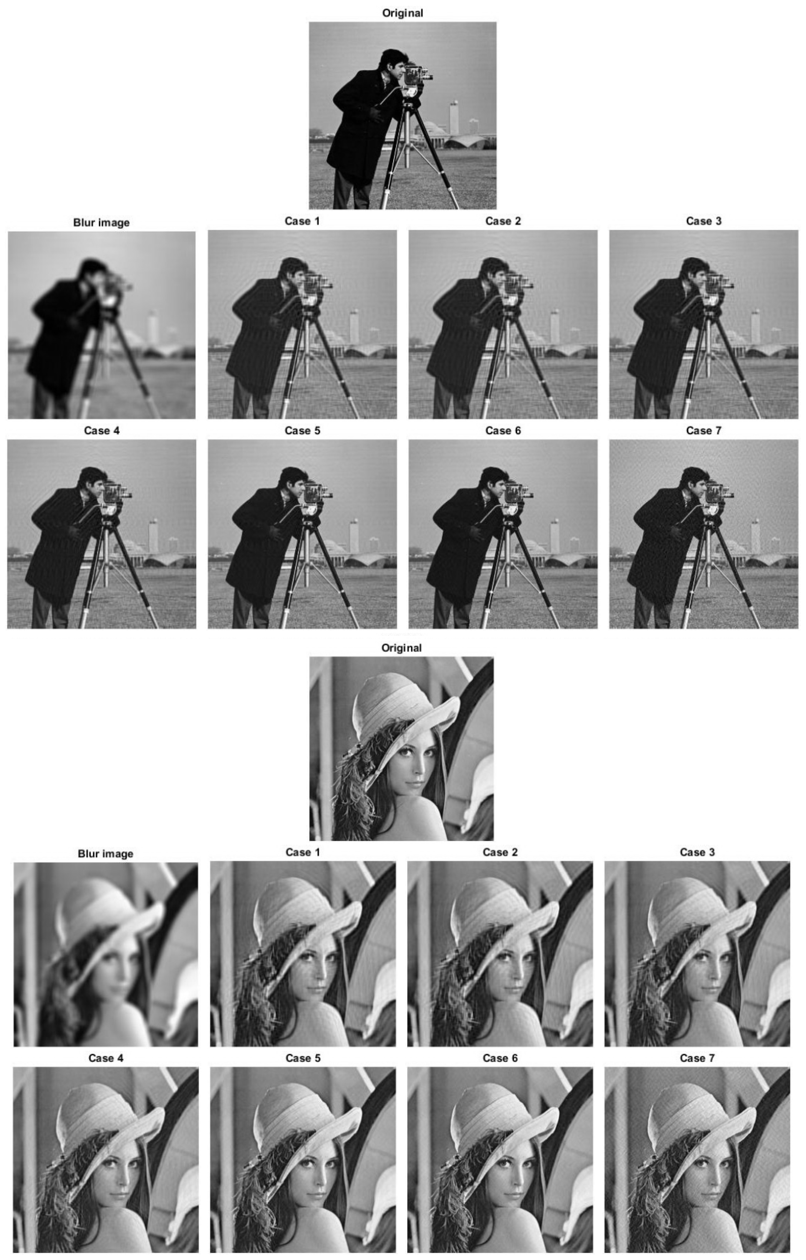
5. Simulated Results for the Image Restoration Problem

In this section, we apply Algorithm 2 (FBMWA) to solving the image restoration problem (2) and compare the deblurring efficiency of the FBMWA algorithm with FBS [30], IFBS [35], FISTA [28] and NAGA [37]. Our programs were written in Matlab and all algorithms ran on a laptop, Intel core i5, 4.00 GB RAM. All algorithms were applied to solving problem (2), where $f\left(y\right)={\parallel Ay-a\parallel }_2^2,$$h\left(y\right)={\lambda \parallel y\parallel }_1,$A is the blurring operator, a is the observed image and $\lambda$ is the regularization parameter.

In this experiment, two gray-scale images, Lenna and Cameraman of size ${256}^2$ are considered the original images. The images went through a Gaussian blur of size $9^2$ and standard deviation $\sigma =4.$ We use the peak signal-to-noise ratio (PSNR) [47] to measure the performance our the algorithms where $PSNR\left(x_n\right)$ is defined by

$$PSNR\left(x_n\right)=10{log}_{10}\left(\frac{{255}^2}{MSE}\right),$$

(19)

where $MSE=\frac{1}{M}{\parallel x_n-\overline{x}\parallel }_2^2,$M is the number of image samples and $\overline{x}$ is the original image. It is noted that a higher value of PSNR of the same number of iteration shows a higher quality of deblurring image. The relative error is defined by

$$\frac{\parallel x_n-x_{n-1}{\parallel }_2}{\parallel x_{n-1}{\parallel }_2}\le tol,$$

(20)

where $tol$ denotes a prescribed tolerance value. For these experiments, the regularization parameter was chosen to be $\lambda =5\times {10}^{-5},$ and the initial image was the blurred image. The Lipschitz constant $L,$ was computed by the maximum eigenvalues of the matrix $A^{T}A.$ We set parameters as follows:

$${\alpha }_n={\beta }_n={\gamma }_n=0.5,c_n=\frac{n}{L(n+1)},c=\frac{1}{L},{\theta }_n\mathrm{defined}\mathrm{by}(6)\left(\mathrm{for}\mathrm{NAGA}\right),$$

$${\theta }_n=\{\begin{array}{cc}\frac{1}{n^2{\parallel x_n-x_{n-1}\parallel }_2^2}\hfill & \mathrm{if}{x}_n\ne x_{n-1},\hfill \\ 0\hfill & \mathrm{otherwise},\hfill \end{array}(\mathrm{for}\mathrm{IFBS}),$$

and

$${\theta }_n=\{\begin{array}{cc}\frac{t_n-1}{t_{n+1}}\hfill & \mathrm{if}1\le n<N,\hfill \\ \frac{1}{2^n}\hfill & \mathrm{otherwise},\hfill \end{array}(\mathrm{for}\mathrm{FBMWA}),$$

where $t_n$ is a sequence defined by $t_1=1$ and $t_{n+1}=\frac{1+\sqrt{1+4t_n^2}}{2},$ and N is a number of iterations that we want to stop. The results of deblurring image of Cameraman and Lenna with 1000th iteration of the studied algorithms are shown in

Table 1. Comparison of image restorations of the studied methods.

	Cameraman		Lenna
Algorithms	PSNR	Tol.	PSNR	Tol.
FBS	27.1953	2.32 × ${10}^{-5}$	29.4907	1.73 × ${10}^{-5}$
IFBS	27.1953	2.32 × ${10}^{-5}$	29.4907	1.73 × ${10}^{-5}$
FISTA	34.6659	4.13 × ${10}^{-5}$	36.9324	3.34 × ${10}^{-5}$
NAGA	35.6670	4.15 × ${10}^{-5}$	37.8088	3.32 × ${10}^{-5}$
FBMWA	36.2783	4.21 × ${10}^{-5}$	38.2989	3.31 × ${10}^{-5}$

and Figure 1 and Figure 2.

From Table 1 and the graph of PSNR in Figure 1, we see that FBMWA gives a higher PSNR than the other algorithms, so the performance of the image restoration of FBMWA is better than those of FBS, IFBS, FISTA and NAGA. We also see that after 1000 iterations, FBMWA gives a better result of deblurring for Cameraman and Lenna, as shown in Figure 2.

The results of deblurring image of Cameraman and Lenna for the 1000th iteration of the FBMWA under different parameters ${\theta }_n$ are shown in

Table 2. Effective parameters of our method for image restoration.

		Cameraman		Lenna
Case	Parameters	PSNR	Tol.	PSNR	Tol.
1	${\mu }_n=\frac{1}{2^n}$	27.8911	2.13 × ${10}^{-5}$	30.1603	1.66 × ${10}^{-5}$
2	${\mu }_n=\frac{10}{n^2}$	27.9003	2.12 × ${10}^{-5}$	30.1693	1.65 × ${10}^{-5}$
3	${\mu }_n=0.5$	28.7146	2.00 × ${10}^{-5}$	30.9771	1.60 × ${10}^{-5}$
4	${\mu }_n=0.9$	30.9920	1.81 × ${10}^{-5}$	33.2838	1.47 × ${10}^{-5}$
5	${\mu }_n=\frac{t_n-1}{t_{n+1}},t_1=1,$ $t_{n+1}=\frac{1+\sqrt{1+4t_n^2}}{2},$	36.2783	4.21 × ${10}^{-5}$	38.2989	3.31 × ${10}^{-5}$
6	${\mu }_n=\frac{n}{n+1}$	37.0979	1.63 × ${10}^{-4}$	38.8562	1.30 × ${10}^{-4}$
7	${\mu }_n=1$	30.6832	9.13 × ${10}^{-4}$	32.7996	7.07 × ${10}^{-4}$

and Figure 3 and Figure 4, where ${\theta }_n$ is defined by

$${\theta }_n=\{\begin{array}{cc}{\mu }_n\hfill & \mathrm{if}1\le n<N,\hfill \\ \frac{1}{2^n}\hfill & \mathrm{otherwise},\hfill \end{array}$$

(21)

where ${\mu }_n$ is a sequence of nonnegative real numbers and N is a number of iterations that we want to stop. We observe that the inertial parameter ${\theta }_n$ using by FBMWA plays an important role in improving quality of deblurring image. It is noted that if $\left\{{\theta }_n\right\}$ is nondecreasing and tends to $1,$ the values of PSNR increase, as shown in Table 2, Figure 3. However, we can see the result of the deblurring image of FBMWA with different inertial parameters ${\theta }_n$ (seven cases), as shown in Figure 4. We also observe from Table 2 that the parameter ${\mu }_n=\frac{n}{n+1}$ gives a higher PSNR than the others.

Open problem: It is noted that we can choose ${\theta }_n$ as in (21) for the Algorithm 2, and convergence of Algorithm 2 can be guaranteed by Theorem 7. Can we use ${\theta }_n$ as defined by (6) for Algorithm 2?

6. Conclusions

In this work, we proposed a modified W-algorithm for solving a common fixed point problem of a family of nonexpansive operators and proved the weak convergence result of the proposed method under some control conditions. We applied our main result to solving a minimization problem in the form of the sum of two proper lower semi-continuous and convex functions. As applications, we applied our algorithm, FBMWA, to solving image restoration problems. Moreover, we did some numerical experiments to illustrate the performance of the studied algorithms and show that PSNR of FBMWA is better than those of the FBS [30], IFBS [35], FISTA [28] and NAGA [37].

References

1. Bauschke, H.H. The approximation of fixed points of compositions of nonexpansive mappings in Hilbert space. J. Math. Anal. Appl. 1996, 202, 150–159. [Google Scholar] [CrossRef] [Green Version]
2. Chidume, C.E.; Bashir, A. Convergence of path and iterative method for families of nonexpansive mappings. Appl. Anal. 2008, 67, 117–129. [Google Scholar] [CrossRef]
3. Halpern, B. Fixed points of nonexpansive maps. Bull. Am. Math. Soc. 1967, 73, 957–961. [Google Scholar] [CrossRef] [Green Version]
4. Ishikawa, S. Fixed points by a new iteration method. Proc. Am. Math. Soc. 1974, 44, 147–150. [Google Scholar] [CrossRef]
5. Klen, R.; Manojlović, V.; Simić, S.; Vuorinen, M. Bernoulli inequality and hypergeometric functions. Proc. Am. Math. Soc. 2014, 142, 559–573. [Google Scholar] [CrossRef]
6. Kunze, H.; La Torre, D.; Mendivil, F.; Vrscay, E.R. Generalized fractal ntransforms and self-similar objects in cone metric spaces. Comut. Math. Appl. 2012, 64, 1761–1769. [Google Scholar] [CrossRef] [Green Version]
7. Mann, W.R. Mean value methods in iteration. Proc. Am. Math. Soc. 1953, 4, 506–510. [Google Scholar] [CrossRef]
8. Radenović, S.; Rhoades, B.E. Fixed point theorem for two non-self mappings in cone metric spaces. Comput. Math. Appl. 2009, 57, 1701–1707. [Google Scholar] [CrossRef] [Green Version]
9. Todorcević, V. Harmonic Quasiconformal Mappings and Hyperbolic Type Metrics; Springer Nature Switzerland AG: Basel, Switzerland, 2019. [Google Scholar]
10. Byrne, C. Iterative oblique projection onto convex subsets and the split feasibility problem. Inverse Probl. 2002, 18, 441–453. [Google Scholar] [CrossRef]
11. Byrne, C. Aunified treatment of some iterative algorithms in signal processing and image reconstruction. Inverse Probl. 2004, 20, 103–120. [Google Scholar] [CrossRef] [Green Version]
12. Cholamjiak, P.; Shehu, Y. Inertial forward-backward splitting method in Banach spaces with application to compressed sensing. Appl. Math. 2019, 64, 409–435. [Google Scholar] [CrossRef]
13. Combettes, P.L.; Wajs, V. Signal recovery by proximal forward–backward splitting. Multiscale Model. Simul. 2005, 4, 1168–1200. [Google Scholar] [CrossRef] [Green Version]
14. Kunrada, K.; Pholasa, N.; Cholamjiak, P. On convergence and complexity of the modified forward-backward method involving new linesearches for convex minimization. Math. Meth. Appl. Sci. 2019, 42, 1352–1362. [Google Scholar]
15. Suantai, S.; Eiamniran, N.; Pholasa, N.; Cholamjiak, P. Three-step projective methods for solving the split feasibility problems. Mathematics 2019, 7, 712. [Google Scholar] [CrossRef] [Green Version]
16. Suantai, S.; Kesornprom, S.; Cholamjiak, P. Modified proximal algorithms for finding solutions of the split variational inclusions. Mathematics 2019, 7, 708. [Google Scholar] [CrossRef] [Green Version]
17. Thong, D.V.; Cholamjiak, P. Strong convergence of a forward–backward splitting method with a new step size for solving monotone inclusions. Comput. Appl. Math. 2019, 38. [Google Scholar] [CrossRef]
18. Censor, Y.; Bortfeld, T.; Martin, B.; Trofimov, A. A unified approach for inversion problems in intensity-modulated radiation therapy. Phys. Med. Biol. 2006, 51, 2353–2365. [Google Scholar] [CrossRef] [Green Version]
19. Censor, Y.; Elfving, T.; Kopf, N.; Bortfeld, T. The multiple set split feasibility problem and its applications. Inverse Probl. 2005, 21, 2071–2084. [Google Scholar] [CrossRef] [Green Version]
20. Censor, Y.; Motova, A.; Segal, A. Perturbed projections and subgradient projections for the multiple-sets feasibility problem. J. Math. Anal. 2007, 327, 1244–1256. [Google Scholar] [CrossRef] [Green Version]
21. Phuengrattana, W.; Suantai, S. On the rate of convergence of Mann, Ishikawa, Noor and SP-iterations for continuousfunctions on an arbitrary interval. J. Comput. Appl. Math. 2011, 235, 3006–3014. [Google Scholar] [CrossRef] [Green Version]
22. Wongyai, S.; Suantai, S. Convergence Theorem and Rate of Convergence of a New Iterative Method for Continuous Functions on Closed Interval. In Proceedings of the AMM and APAM Conference Proceedings, Bankok, Thailand, 23–25 May 2016; pp. 111–118. [Google Scholar]
23. Ben-Tal, A.; Nemirovski, A. Lectures on Modern Convex Optimization, Analysis, Algorithms, and Engineering Applications; MPS/SIAM Ser. Optim.; SIAM: Philadelphia, PA, USA, 2001. [Google Scholar]
24. Bioucas-Dias, J.; Figueiredo, M. A new TwIST: Two-step iterative shrinkage/thresholding algorithms for image restoration. IEEE Trans. Image Process. 2007, 16, 2992–3004. [Google Scholar] [CrossRef] [PubMed] [Green Version]
25. Chen, S.S.; Donoho, D.L.; Saunders, M.A. Atomic decomposition by basis pursuit. SIAM J. Sci. Comput. 1998, 20, 33–61. [Google Scholar] [CrossRef]
26. Donoho, D.L.; Johnstone, I.M. Adapting to unknown smoothness via wavelet shrinkage. J. Am. Statist. Assoc. 1995, 90, 1200–1224. [Google Scholar] [CrossRef]
27. Figueiredo, M.A.T.; Nowak, R.D.; Wright, S.J. Gradient projection for sparse reconstruction: Application to compressed sensing and other inverse problems. IEEE J. Sel. Top. Signal Process. 2007, 1, 586–597. [Google Scholar] [CrossRef] [Green Version]
28. Beck, A.; Teboulle, M. A fast iterative shrinkage-thresholding algorithm for linear inverse problems. SIAM J. Imaging Sci. 2009, 2, 183–202. [Google Scholar] [CrossRef] [Green Version]
29. Tibshirani, R. Regression shrinkage and selection via the lasso. J. R. Stat. Soc. B Methodol. 1996, 58, 267–288. [Google Scholar] [CrossRef]
30. Lions, P.L.; Mercier, B. Splitting algorithms for the sum of two nonlinear operators. SIAM J. Numer. Anal. 1979, 16, 964–979. [Google Scholar] [CrossRef]
31. Moreau, J.J. Proximité et dualité dans un espace hilbertien. Bull. Soc. Math. Fr. 1965, 93, 273–299. [Google Scholar] [CrossRef]
32. Figueiredo, M.A.T.; Nowak, R.D. An EM algorithm for wavelet-based image restoration. IEEE Trans. Image Process. 2003, 12, 906–916. [Google Scholar] [CrossRef] [Green Version]
33. Daubechies, I.; Defrise, M.; Mol, C.D. An iterative thresholding algorithm for linear inverse problems with a sparsity constraint. Commun. Pure Appl. Math. 2004, 57, 1413–1457. [Google Scholar] [CrossRef] [Green Version]
34. Hale, E.T.; Yin, W.; Zhang, Y. A Fixed-Point Continuation Method for l1-Regularized Minimization. Siam J. Optim. 2008, 19, 1107–1130. [Google Scholar] [CrossRef]
35. Moudafi, A.; Oliny, M. Convergence of a splitting inertial proximal method for monotone operators. J. Comput. Appl. Math. 2003, 155, 447–454. [Google Scholar] [CrossRef] [Green Version]
36. Liang, J.; Schonlieb, C.B. Improving fista: Faster, smarter and greedier. arXiv 2018, arXiv:1811.01430. [Google Scholar]
37. Verma, M.; Shukla, K.K. A new accelerated proximal gradient technique for regularized multitask learning framework. Pattern Recogn. Lett. 2017, 95, 98–103. [Google Scholar] [CrossRef]
38. Nakajo, K.; Shimoji, K.; Takahashi, W. Strong convergence to common fixed points of families of nonexpansive mappings in Banach spaces. J. Nonlinear Convex Anal. 2007, 8, 11–34. [Google Scholar]
39. Nakajo, K.; Shimoji, K.; Takahashi, W. On strong convergence by the hybrid method for families of mappings in Hilbert spaces. Nonlinear Anal. Theor. Methods Appl. 2009, 71, 112–119. [Google Scholar] [CrossRef]
40. Boyd, S.; Vandenberghe, L. Convex Optimization; Cambridge University Press: New York, NY, USA, 2004. [Google Scholar]
41. Bauschke, H.H.; Combettes, P.L. Convex Analysis and Monotone Operator Theory in Hilbert Spaces; Springer: New York, NY, USA, 2011. [Google Scholar]
42. Burachik, R.S.; Iusem, A.N. Set-Valued Mappings and Enlargements of Monotone Operator; Springer Science Business Media: New York, NY, USA, 2007. [Google Scholar]
43. Bussaban, L.; Suantai, S.; Kaewkhao, A. A parallel inertial S-iteration forward-backward algorithm for regression and classification problems. Carpathian J. Math. 2020, 36, 21–30. [Google Scholar]
44. Takahashi, W. Introduction to Nonlinear and Convex Analysis; Yokohama Publishers: Yokohama, Japan, 2009. [Google Scholar]
45. Tan, K.; Xu, H.K. Approximating fixed points of nonexpansive mappings by the ishikawa iteration process. J. Math. Anal. Appl. 1993, 178, 301–308. [Google Scholar] [CrossRef] [Green Version]
46. Moudafi, A.; Al-Shemas, E. Simultaneous iterative methods for split equality problem. Trans. Math. Program. Appl. 2013, 1, 1–11. [Google Scholar]
47. Thung, K.; Raveendran, P. A survey of image quality measures. In Proceedings of the International Conference for Technical Postgraduates (TECHPOS), Kuala Lumpur, Malaysia, 14–15 December 2009; pp. 1–4. [Google Scholar]
Figure 1. The graphs of peak signal-to-noise ratio (PSNR) for Cameraman (left) and Lenna (right).
Mathematics 08 00378 g001
Figure 2. Results for deblurring of the Cameraman and Lenna.
Mathematics 08 00378 g002
Figure 3. The graphs of PSNR of the FBMWA under different parameters θ n for Cameraman (left) and Lenna (right).
Mathematics 08 00378 g003
Figure 4. Results of FBMWA for deblurring of the Cameraman and Lenna.
Mathematics 08 00378 g004