On the Smoothing of the Generalized Extreme Value Distribution Parameters Using Penalized Maximum Likelihood: A Case Study on UVB Radiation Maxima in the Mexico City Metropolitan Area

Abstract

This paper concerns the use and implementation of penalized maximum likelihood procedures to fitting smoothing functions of the generalized extreme value distribution parameters to analyze spatial extreme values of ultraviolet B (UVB) radiation across the Mexico City metropolitan area in the period 2000–2018. The model was fitted using a flexible semi-parametric approach and the parameters were estimated by the penalized maximum likelihood (PML) method. In order to investigate the performance of the model as well as the estimation method in the analysis of complex nonlinear trends for UVB radiation maxima, a simulation study was conducted. The results of the simulation study showed that penalized maximum likelihood yields better regularization to the model than the maximum likelihood estimates. We estimated return levels of extreme UVB radiation events through a nonstationary extreme value model using measurements of ozone (O₃), nitrogen oxides (NO_x), particles of 10 μm or less in diameter (PM₁₀), carbon monoxide (CO), relative humidity (RH) and sulfur dioxide (SO₂). The deviance statistics indicated that the nonstationary generalized extreme value (GEV) model adjusted was statistically better compared to the stationary model. The estimated smoothing functions of the location parameter of the GEV distribution on the spatial plane for different periods of time reveal the existence of well-defined trends in the maxima. In the temporal plane, a presence of temporal cyclic components oscillating over a weak linear component with a negative slope is noticed, while in the spatial plane, a weak nonlinear local trend is present on a plane with a positive slope towards the west, covering the entire study area. An explicit spatial estimate of the 25-year return period revealed that the more extreme risk levels are located in the western region of the study area.

1. Introduction

Ultraviolet radiation can cause different effects on Earth’s life. In living organisms, UVB radiation destroys DNA, produces protein denaturation, triggers coagulation of albumin, as well as erythema and skin problems. In humans, UVB radiation causes the weakening of immune system, creates conditions for the development of skin cancer, cataract, aging as well as the formation of erythema [1], dealing to wide economic losses in public health and thousands of deaths each year due to skin cancer [2].

The intensity of UVB radiation at ground level is affected by the absorption of energy required by the chemical reactions that occur in the atmosphere and by the reflection caused by particles and gases. One of the most important is ozone, which among all atmospheric gases plays an active role in the absorption of UV radiation and protection against dangerous levels of solar radiation [3]. In the stratosphere, UVB is absorbed mainly in the ozone layer. This region concentrates ninety percent of total ozone at an altitude of between 9 to 18 miles forming a protective shield against UVB radiation. The ozone concentration varies spatially due to chemical reactions which constantly create or destroy this element. In densely populated areas with air pollution problems, UVB radiation interacts with pollutant oxides of nitrogen and nonmethane hydrocarbons in the troposphere to form ozone. There are other air pollutants called ozone-depleting substances (ODS) which, in contact with UVB radiation, release chemical compounds such as chlorine and bromine, which destroy the ozone in the stratosphere. In all latitudes, except the equatorial zone, from 1979 to 1998, the decrease in ozone was the cause of the annual average increase in ultraviolet radiation from 290 nm to 325 nm [4].

The relationships between ultraviolet radiation and air pollutants have been widely used to analyze the spatial distribution of continuous levels of UVB radiation through statistical models [5]. The covariates that have been used by these models to explain the spatial and temporal distribution of UVB radiation are clouds, ozone, nitrogen oxides, particulate matter, carbon monoxide and sulfur dioxide [6]. The clouds have an effect on the distribution of UVB radiation. Scattering by clouds increases the rate of photochemical reactions and reduces the radiation below them. The particulate matter concentration is also an important factor that plays an important role in the distribution of ultraviolet radiation. In [7], Sun et al. showed that the magnitude of correlation between PM_2.5 and ultraviolet radiation is of the order of −0.5 in the near-surface layer. They deduced that the maximum and the daily average UV radiations could be attenuated by particulate matter by 40% at most. Their results showed that if one day the average UV radiation was high, the next day the average UV radiation was also high, the reason was that the amount of chemical reactions related to UV radiation created new particulate material. Fluctuations of intensities in ultraviolet radiation are also caused by the amounts of atmospheric NO₂ and SO₂. In [8], McKenzie et al. found that if the amount of NO₂ is increased 10 or more times than the average amount, then the irradiation of UVA rays decreases up to 40.

One of the most important results of statistical theory were developed by Fisher and Tippett [9], and Gnedenko [10] on the asymptotic distribution of the maximum of a random sample. They showed that if the maximum of a random sample centered and scaled by properly chosen constants converges to some distribution, it should be one of the following: Fréchet, Weibull or Gumbel. Later, Jenkinson [11] combined these three distributions into a single distribution, known as the generalized extreme value distribution, also known as the generalized extreme value (GEV) distribution. The GEV distribution uses three parameters corresponding to the location, scale and shape. The sign of the shape parameter determines the type of the distribution: negative values correspond to the Weibull, positive values to the Fréchet and zero to the Gumbel distribution. The estimation of the parameters has been made using maximum likelihood [12,13], partial probability weighted moments, L-moments [14] as well as several Bayesian approaches [15,16]. The L-moments estimators are sometimes more accurate in small samples than those obtained by maximum likelihood and in the case of outliers in the data, are more robust than the conventional moments methods [17,18]. Martins and Stedinger [19] showed that the method of penalized maximum likelihood provided better estimates than maximum likelihood and method of moments when the sample sizes are small and the GEV distribution has heavy-tailed tails.

The generalized distribution of extreme values was developed under the assumption of independent samples with stationary distribution. However, since most real applications have spatial or temporal trends, it has been adapted for the study of nonstationary processes [20]. The nonstationary extreme value analysis has been widely used to study extreme events in hydrology, hydroclimatology, as well as in environmental, anthropogenic and geophysical processes. Particularly, it has been used to study the long-term risks in rainfall [21], winds [22], heat waves [16] and earthquakes [23,24]. In these studies, it can be seen that the trend of extreme values has been adjusted using several approaches. In fact, one of these approaches is that if the patterns follow the law determined by a model, then the GEV parameters of the corresponding model are estimated [25,26]. In contrast, for some others, it is more appropriate to adjust the trend with smoothing functions [21,27]. In both cases, the trend is adjusted by estimating the parameters on predictors of the location parameter of the GEV distribution. Analogously, an adjustment similar to the logarithm of the scale parameter is made [28,29,30]. The contrast occurs for the shape parameter, which is assumed to be constant because the estimation is numerically fraught when this parameter is allowed to be too flexible [28]. Extreme nonstationary values have also been studied extensively using the Bayesian approach. For instance, Gaetan and Grigoletto [15] studied rainfall maxima with Markov random fields approximated based on smoothing kernel, Reich et al. [16] studied heat waves using a Bayesian hierarchical model with the generalized Pareto distribution (GPD) and Sang and Gelfand [31] studied the extreme values of spatial stochastic processes and modeled the observed trend as a function of spatial covariates.

2. Methods

2.1. Study Area

The Mexico City metropolitan area (MCMA) is one of the largest urban area of the world, with nearly $25.4$ million people distributed in about $9560{\mathrm{km}}^2$. The MCMA is composed by the Mexico City, 59 municipalities of the state of Mexico and one municipality of the state of Hidalgo. The MCMA is located within a raised basin at an average elevation of 2240 m surrounded by mountains to the east, south and west. The topography combined with meteorological phenomena modify pollutant dispersion pattern. The study area and the primary sampling sites located in FES Acatlán (FAC), Hangares (HAN), Merced (MER), Montecillo (MON), Pedregal (PED), San Agustín (SAG), Santa Fe (SFE) and Tlalnepantla (TLA) are shown in Figure 1.

2.2. Methodology

A Nonstationary GEV Model

Inferences about the parameters of the extreme values can be made with the exact distribution of the maximum of a random sample when the cumulative distribution function of the target population is known. However, in large samples the exact distribution function tends to concentrate the mass of the probabilities in a single point, known as degenerate distribution. This kind of distribution is not useful for further analysis. In other cases neither the population distribution is known, nor the sample is small. One solution to these limitations is to approximate the asymptotic distribution of the extremes through the limit distribution of a properly rescaled sequence. Consider $Y_1,...,Y_n$ a sample of independent and identically distributed random variables with cumulative distribution function $F_Y\left(y\right)$ and let $M_n=$ max $\left(Y_1,...,Y_n\right)$, then the only limiting nondegenerate distribution $G_n=(M_n-a_n)/b_n$ as $n\to \infty$ (if such a sequences of constants $\left\{b_n\right\}$ and $\left\{a_n\right\}$ such that for each $n\in \mathbb{N}$, $b_n>0$ exist) is the generalized extreme value (GEV) distribution [11]:

$$G\left(y\right)=\left\{\begin{array}{cc}exp\left\{-{\left(1+\kappa \frac{\left(y-\mu \right)}{\sigma }\right)}^{-\frac{1}{\kappa }}\right\},\hfill & \kappa \ne 0\hfill \\ exp\left\{-exp\left(-\frac{(y-\mu )}{\sigma }\right)\right\},\hfill & \kappa =0\hfill \end{array}\right.$$

for $y:1+\kappa \frac{\left(y-\mu \right)}{\sigma }>0$ when $\kappa \ne 0$, where $-\infty \le y\le \mu -\sigma /\kappa$ when $\kappa <0$ (Weibull), $\mu -\sigma /\kappa \le y\le +\infty$ when $\kappa >0$ (Fréchet) and $-\infty \le y\le +\infty$ when $\kappa =0$ (Gumbel). Here, $\mu \in \mathbb{R}$, $\sigma >0$ and $\kappa \in \mathbb{R}$ are the location, scale and shape parameters, respectively. The quantile function of the GEV distribution, obtained with $Q\left(p\right)=G^{-1}\left(p\right)$, is given by

$$\begin{array}{c}\hfill Q\left(p\right)=\left\{\begin{array}{cc}\mu +\frac{\sigma }{\kappa }\left[{\left[-log\left(p\right)\right]}^{-\kappa }-1\right],\hfill & \kappa \ne 0\hfill \\ \mu -\sigma log\{-log(p\left)\right\},\hfill & \kappa =0\hfill \end{array}\right.\end{array}$$

(1)

The GEV distribution was derived using the stationarity assumption inherited from a random sample. In a real scenario, the maxima are usually not identically distributed, i.e., the mean of the distribution varies as a function of covariates. In such cases, we establish a predictor to the parameters of location, scale and shape of the form ${\mu }_t=\mu \left(X_{t1},...,X_{tk}\right)$, ${\sigma }_t=\sigma \left(X_{t1},...,X_{tk}\right)$ and ${\kappa }_t=\kappa \left(X_{t1},...,X_{tk}\right)$ [20].

2.3. Proposed Approach

Similar to the approach of generalized linear vector models proposed by Yee and Stephenson [28] and the analysis of nonstationary extreme values proposed by Coles [20], we associated a linear predictor to the parameters of the GEV distribution. The linear predictor expresses the relationship of a set of covariates with the maxima through the parameters, which usually consists of linear functions. The structure of the linear predictor is analogous to linear regression models based on spline-based functions. However, the regression is not directly done on the response variable, but is assigned a linear function with a radial basis kernel to approximate the trend of UVB radiation maxima through the location parameter. We chose a flat function for the scale and shape parameter respectively, because the estimation is numerically fraught when this parameters are allowed to be too flexible. Therefore, the proposed model is as follows:

$$\begin{array}{cc}\hfill {\mu }_t& =c_0+x_{t1}{c}_1+\dots +x_{t\left(p_1-1\right)}{c}_{p_1-1}+exp\left(\left(\varphi {∥{\underline{x}}_i-{\underline{k}}_1∥}^2\right)\right)d_1+\dots +exp\left(\left(\varphi {∥{\underline{x}}_i-{\underline{k}}_{p_2}∥}^2\right)\right)d_{p_2},\hfill \\ \hfill {\kappa }_t& =\kappa ,\hfill \\ \hfill log{\sigma }_t& =v,\hfill \end{array}$$

(2)

where $\varphi \left(·\right)$ is a real value function, ${\sigma }_t$, $\kappa$ and ${\mu }_t$ are scale, shape and location parameters, respectively, ${\underline{x}}_t=\left[x_{t1},\dots ,x_{t\left(p_1-1\right)}\right]$ is the vector of covariates for the t-th observation, scaled and centered, and ${\underline{k}}_j$ corresponds to the j-th centroid obtained by the method of hierarchical clustering among ${\underline{x}}_t,t=1.2,\dots ,n$ [32]. Note that the set of location parameter can be expressed in matrix notation as $\mu =X{\beta }_{\left(1\right)}+Z{u}_{\left(1\right)}$ where ${\beta }_{\left(1\right)}^{\top }=\left[c_0,c_1,\dots ,c_{p_1-1}\right]$ is a vector of size $p_1$, $u_{\left(1\right)}^{\top }=\left[d_1,\dots ,d_{p_2}\right]$ is a vector of size $p_2$, X is a $n\times p_1$ matrix which has the additional column of one for the coefficient of $c_0$ and ${\left[Z_{ij}\right]}^{\top }={\left[exp\left(\varphi \left({∥{\underline{x}}_i-{\underline{k}}_j∥}^2\right)\right)\right]}^{\top }$ is a $p_2\times n$ matrix of kernel basis which consists of a set of columns obtained by using radial Gaussian function used to approximate the trend and capture the interactions between covariates.

Penalized Maximum Likelihood

Let $\underline{y}=(y_1,...,y_n)$ be a sample of n extremes. The maximum likelihood estimator for the nonstationary GEV is defined as the estimator that maximizes the joint density of the n random variables:

$$\begin{array}{ccc}\hfill L({\mu }_t,{\sigma }_t,{\kappa }_t\mid \underline{y})& =& \prod _{t=1}^n\frac{1}{{\sigma }_t}exp\left\{-{\left[1+{\kappa }_t\left(\frac{y_t-{\mu }_t}{{\sigma }_t}\right)\right]}^{-\frac{1}{{\kappa }_t}}\right\}\times {\left[1+{\kappa }_t\left(\frac{y_t-{\mu }_t}{{\sigma }_t}\right)\right]}_{.}^{-\left(1+\frac{1}{{\kappa }_t}\right)}\hfill \end{array}$$

It can be seen that maximizing the likelihood function with respect of the GEV parameters is equivalent to maximizing the log-likelihood function:

$$\begin{array}{c}\hfill \ell ({\mu }_t,{\sigma }_t,\kappa \mid \underline{y})=-nlog{\sigma }_t-\sum _{t=1}^n{\left[1+\kappa \left(\frac{y_t-{\mu }_t}{{\sigma }_t}\right)\right]}^{-\frac{1}{\kappa }}-\sum _{t=1}^n\left(1+\frac{1}{\kappa }\right)log{\left[1+\kappa \left(\frac{y_t-{\mu }_t}{{\sigma }_t}\right)\right]}_{.}\end{array}$$

Let $C=\left[XZ\right]$ and ${\underline{b}}_{\left(1\right)}^{\top }=\left[{\underline{\beta }}_{\left(1\right)}^{\top }{\underline{u}}_{\left(1\right)}^{\top }\right]$, where C is an $n\times p$ matrix, with $p=p_1+p_2$; ${\underline{b}}_{\left(1\right)}$ is a vector of $p\times 1$ parameters, the linear predictor of the location parameter can be written as $\mu =C{\underline{b}}_{\left(1\right)}$. The penalty of the parameters is introduced through the following matrix:

$$P_1=\left[\begin{array}{cc}\frac{1}{{\sigma }_{\beta }^2}{I}_{p_1}& 0\\ 0& \frac{1}{{\sigma }_u^2}\left[\left(I_{P_2}+D_d^{\top }{D}_d\right)\right]\end{array}\right];P_2=\left[\begin{array}{cc}\frac{1}{{\sigma }_v^2}& 0\\ 0& \frac{1}{{\sigma }_{\kappa }^2}\end{array}\right]$$

where $I_{p_1}$ and $I_{p_2}$ are identity matrices of order $p_1$ and $p_2$ respectively, ${\sigma }_{\beta }^2$, ${\sigma }_u^2$, ${\sigma }_v^2$ and ${\sigma }_{\kappa }^2$ are values that control the degree of shrinkage on coefficient estimates and $D_d{\underline{u}}_1={\Delta }^d{\underline{u}}_1$ consists of the vector of $dth$ differences of ${\underline{u}}_1$.

Therefore the penalized log-likelihood of the model is:

$$\begin{array}{c}\hfill {\ell }_n^p({\mu }_t,{\sigma }_t,\kappa \mid \underline{y})=\sum _{t=1}^n{\ell }_t({\mu }_t,{\sigma }_t,\kappa \mid \underline{y})-{\underline{b}}_{\left(1\right)}^{\top }{P}_1{\underline{b}}_{\left(1\right)}-w^{\top }{P}_{2}w\end{array}$$

(3)

where ${\ell }_t({\mu }_t,{\sigma }_t,\kappa \mid \underline{y})=-log{\sigma }_t-{\left[1+\kappa \left(\frac{y_t-{\mu }_t}{{\sigma }_t}\right)\right]}^{\frac{1}{\kappa }}log\left[1+\kappa \left(\frac{y_t-{\mu }_t}{{\sigma }_t}\right)\right]$ and $w=\left[v,\kappa \right]$. Defining ${\ell }_n({\mu }_t,{\sigma }_t,\kappa \mid \underline{y})$ = ${\displaystyle \sum _{t=1}^n}{\ell }_t({\mu }_t,{\sigma }_t,\kappa \mid \underline{y})$ and ${\ell }_{PL}({\underline{b}}_{\left(1\right)},{\sigma }_t,\kappa )$ = $\left[-{\underline{b}}_{\left(1\right)}^{\top }{P}_1{\underline{b}}_{\left(1\right)}-w^{\top }{P}_{2}w\right]$, we can rewrite the Equation (3) as:

$$\begin{array}{c}\hfill {\ell }_n^p({\mu }_t,{\sigma }_t,\kappa \mid \underline{y})={\ell }_n({\mu }_t,{\sigma }_t,\kappa \mid \underline{y})+{\ell }_{PL}{(b_{\left(1\right)},{\sigma }_t,\kappa )}_{.}\end{array}$$

(4)

The gradient of the likelihood is given by:

$$\frac{\partial {\ell }_n^p({\mu }_t,{\sigma }_t,\kappa \mid \underline{y})}{\partial b_1}=\sum _{t=1}^n\frac{\partial {\ell }_t({\mu }_t,{\sigma }_t,\kappa \mid \underline{y})}{\partial {\mu }_t}{\underline{c}}_t-2{\underline{b}}_{\left(1\right)}^{\top }{P}_1.$$

$$\frac{\partial {\ell }_n^p({\mu }_t,{\sigma }_t,\kappa \mid \underline{y})}{\partial v}=\sum _{t=1}^n\frac{\partial {\ell }_t({\mu }_t,{\sigma }_t,\kappa \mid \underline{y})}{\partial v}-\frac{2v}{{\sigma }_v^2}$$

$$\frac{\partial {\ell }_n^p({\mu }_t,{\sigma }_t,\kappa \mid \underline{y})}{\partial \kappa }=\sum _{t=1}^n\frac{\partial {\ell }_t({\mu }_t,{\sigma }_t,\kappa \mid \underline{y})}{\partial \kappa }-\frac{2\kappa }{{\sigma }_{\kappa }^2},$$

where ${\underline{c}}_t^{\top }=\left[{\underline{x}}_t^{\top },{\underline{z}}_t^{\top }\right]$. The Hessian matrix is given by $H={\displaystyle \sum _{t=1}^n}{H}_{\left(t\right)}$ as follow:

$$H_{\left(t\right)}=\left[\begin{array}{cc}{H}_{1\left(t\right)}& H_{2\left(t\right)}\\ H_{2\left(t\right)}^{\top }& H_{3\left(t\right)}\end{array}\right].$$

Considering ⊗ as the usual Kronecker product, the elements of the Hessian matrix are:

$$\begin{array}{cc}\hfill H_{1\left(t\right)}& =\frac{\partial {\ell }_t({\mu }_t,{\sigma }_t,\kappa \mid \underline{x})}{\partial {\mu }_t^2}\otimes {\underline{c}}_t{\underline{c}}_t^{\top }-2P_1\hfill \\ \hfill H_{2\left(t\right)}^{\top }& =\left[\begin{array}{c}\frac{\partial {\ell }_t({\mu }_t,{\sigma }_t,\kappa \mid \underline{x})}{\partial {\mu }_t\partial v}\\ \frac{\partial {\ell }_t({\mu }_t,{\sigma }_t,\kappa \mid \underline{x})}{\partial {\mu }_t\partial \kappa }\end{array}\right]\otimes {\underline{c}}_t^{\top }\hfill \\ \hfill H_{3\left(t\right)}& =\left[\begin{array}{cc}\frac{\partial {\ell }_t({\mu }_t,{\sigma }_t,\kappa \mid \underline{x})}{\partial v^2}& \frac{\partial {\ell }_t({\mu }_t,{\sigma }_t,\kappa \mid \underline{x})}{\partial v\partial \kappa }\\ \frac{\partial {\ell }_t({\sigma }_t,{\kappa }_t,\kappa \mid \underline{x})}{\partial v\partial \kappa }& \frac{\partial {\ell }_t({\mu }_t,{\sigma }_t,\kappa \mid \underline{x})}{\partial {\kappa }^2}\end{array}\right]-2P_2\hfill \end{array}$$

We can observe that the gradient and Hessian equations have been expressed in terms of those derived from the density function of the response variable, in this case the GEV distribution. Thus, we considered this formulation to be advantageous because these expressions could be used analogously in different smoothing models with penalties that have a linear predictor similar to Equation (2).

2.4. Simulation Study

In order to examine the performance of the semi-parametric GEV model defined in Equation (2), a simulation study was conducted. The nonlinear system that is addressed by Equation (5) was used to simulate the trend of $n=500$ extreme values sampled from a nonstationary GEV distribution. In this function, $x_1$ and $x_2$, correspond to the longitude and latitude, respectively. To perform a more realistic simulation, the intervals for $x_1$ and $x_2$ were chosen on the current range of the UVB radiation data. Therefore, the $x_1$ values were generated with randomly spaced data on the interval $\left[\mathrm{98.88.99.38}\right]$, and the values of the covariate $x_2$ were randomly selected from the interval $\left[\mathrm{19.15.19.73}\right]$, with

$$\begin{array}{cc}\hfill & {\mu }_t=5+\frac{25}{6\pi }\left[e^{\left[\frac{1}{2}{\left[{\left(x_1-99.22\right)}^2+{\left(x_2-19.34\right)}^2\right]}^{\frac{1}{3}}\right]}-e^{\left[\frac{1}{2}{\left[{\left(x_1-99.05\right)}^2+{\left(x_2-19.54\right)}^2\right]}^{\frac{1}{3}}\right]}\right]\hfill \\ \hfill & {\sigma }_t=\sigma =0.1\hfill \\ \hfill & {\kappa }_t=\kappa =-0.4\hfill \end{array}$$

(5)

The performance of proposed model was evaluated through the simulation of a simple function which consists of two critical points where the function has a maximum and minimum, respectively. We simulated the data using the inverse transform method proposed by Ross [33] as follows: (1) we generated random values for $x_1$ and $x_2$ and obtained ${\mu }_t$, $\sigma$ and $\kappa$, using Equation (5); (2) we generated a random value q with uniform distribution and (3) simulated values were obtained through the inverse of the GEV distribution, given by the Equation (1), using the value of q obtained in step 2 and the values of ${\mu }_t$, $\sigma$ and $\kappa$ obtained in step 1. Regarding the number of knots, we consider two settings, the first one using a set of basis functions with $p_2=20$ knots and the second with $p_2=80$ knots, in both cases we choose ${\sigma }_{\beta }^2=1$, ${\sigma }_u^2=1$, ${\sigma }_v^2=1$ and ${\sigma }_{\kappa }^2=1$. We can see in Figure 2, that the log-likelihood has stabilized at settings $p_2=80$. Once the model was estimated, the estimates obtained for the shape parameter were −0.4000 and −0.4016, respectively. The estimate of the scale parameter was 0.1000 and 0.1002, respectively. The true functions of $\mathsf{\mu }$ expressed as a function of the covariates $x_1$ and $x_2$ are shown in Figure 3a. The function corresponding to $\mathsf{\mu }$ involves the sum of the exponentials to the square of the covariates $x_1$ and $x_2$, which represents a nonlinear surface in the spatial plane, similar to the conditions in the extreme values that can occur in real situations of nonstationary extreme values. As expected, Figure 3c shows that the estimation improved by increasing the number of knots in the spline functions. The function for $\sigma$ and $\kappa$ are constant in the covariate space.

The goodness of fit for the proposed model using the simulated data was evaluated using the mean square error (RMSE) and Pearson’s correlation, given by Equations (6) and (7). We simulated a new data set of 500 observations of model in Equation (2) and then calculated the RMSE with respect to their estimated values. For the location parameter, in the model with $k=80$, we obtained a RMSE of 0.0788 and a correlation of 0.9949 between the predicted values and the testing data. Regarding the interpretation of the coefficients, due to the nonlinear form of the estimated function, the estimated coefficients of the spline model cannot be interpreted directly as marginal changes of the covariates, however, we can still analyze the adjusted function in the covariable space and obtain enough information about the behavior of the trend of extreme values for different values of the covariates.

$$\begin{array}{c}\hfill \mathrm{RMSE}=\sqrt{\frac{{{\displaystyle \sum _{t=1}^n}\left({\mu }_t-{\widehat{\mu }}_t\right)}^2}{n}}\end{array}$$

(6)

$$\begin{array}{c}\hfill \mathrm{Pearson}’\mathrm{s}\mathrm{correlation}=\frac{{\displaystyle \sum _{t=1}^n}\left({\mu }_t-{\overline{\mu }}_t\right)\left({\widehat{\mu }}_t-{\overline{\widehat{\mu }}}_t\right)}{{\sigma }_{{\mu }_t}{\sigma }_{{\widehat{\mu }}_t}}\end{array}$$

(7)

where ${\mu }_t$ is the t-th simulated trend, ${\widehat{\mu }}_t$ is its corresponding estimate; ${\overline{\mu }}_t$ and ${\overline{\widehat{\mu }}}_t$ are the means of the set of simulated and estimated values, respectively; and ${\sigma }_{{\mu }_t}$ and ${\sigma }_{{\widehat{\mu }}_t}$ are their corresponding standard deviations.

An inspection of the estimated functions presented in Figure 3 show that the proposed model with both $p_2=20$ and $p_2=80$ recovers the original form of the real function used in the simulation. In the case of the estimated smoothing function build with 20 knots, i.e., $p_2=20$, we observed a more pronounced border effect, similar to the case of spline functions when the response variable has a normal distribution. This border effect is visibly reduced as we increased the number of nodes, in the model with $k=80$ of Figure 3c, in which we graphically observed that the shape of the estimated function is more similar to the true function Figure 3a. Similarly, a comparison of estimators of $\sigma$ in both $p_2=20$ and $p_2=80$ reveals that the estimation of the scale parameter of the extreme values based on the model given in Equation (2) improves in the case when the number of nodes is increased when $k=80$. In contrast, the estimators of the shape parameter are slightly skewed to the right in both cases.

2.5. Data Description

The data corresponded to 397 observations of bi-monthly maxima of UVB radiation and its corresponding atmospheric covariates, obtained between 1 January 2000, and 30 September 2018, at 7 fixed monitoring stations of the Red Automática de Monitoreo Atmosférico, RAMA (http://www.aire.cdmx.gob.mx/default.php). This monitoring network subsystem is one of the three subsystems of the Sistema de Monitoreo Atmosférico (SIMAT) established by the Comision Ambiental Metropolitana of Mexico City to monitor compliance with ambient air quality standards. The information obtained by the measuring instruments of the RAMA network is concentrated in a computer that sends the information continuously through the modem to the Control Center. The gases are measured in real time, by different methods. O₃ is measured by photometry in the ultraviolet range; NO_x by chemiluminescence; CO by nondispersive spectroscopy by correlation; relative humidity is measured using a sensor, capacitor-type, of polymer thin film.

2.6. Data Analysis

The extreme values were obtained from space–time using the block maxima methodology. The statistical analysis was performed using the $R\mathrm{3.4.2}$ software [34]. In the spatial plane, we considered each station as a block, a total of 7 stations were used. In the temporal plane, the width of the time interval was two months. Due to problems in the measurement instruments, we identified 195 records which had missing data in any of the covariates associated with a maximum of radiation. These observations were excluded from the study. We estimated a GEV model for the maxima of UVB radiation on the Mexico City metropolitan area using a multivariate smoothing functions with spatio-temporal and environmental covariates like latitude (${\mathrm{s}}_1$), longitude (${\mathrm{s}}_2$), time (t), ozone (O₃), nitrogen oxides (NO_x), carbon monoxide (CO), relative humidity (RH), particulate matter of 10 μm or less in diameter are called PM₁₀ (PM₁₀) and sulfur dioxide (SO₂), grouped into the X matrix to fit the trends in the nonstationary GEV model. In order to avoid abrupt changes between the coefficients, we assign a $P=\frac{1}{{\sigma }_1^2}\left(I_{P_2}+D_d^{\prime }{D}_d\right)$ penalty matrix to the coefficients $u_1^{\prime }s$ in the model in Equation (4), where $D_d$ (with $d=1$) is a matrix such that $D_d{u}_1={\Delta }^d{u}_1$ constructs the vector of $dth$ differences of $u_1$.

3. Results and Discussion

The descriptive statistics of the data by each monitoring station are shown in

Table 1. Descriptive summary information on the UVB radiation maxima on the Mexico City metropolitan area.

ID	Name	Simbol	Long $\left(\mathit{W}\right)$	Lat $\left(\mathit{N}\right)$	Min.	1st Qu.	Median	Mean	3rd Qu.	Max.
1	FES Acatlán	FAC	−99${}^{\circ }$14′36.68″	19${}^{\circ }$28′56.90″	4.04	5.18	5.35	5.3	5.55	6.09
2	Hangares	HAN	−99${}^{\circ }$05′01.04″	19${}^{\circ }$25′13.86″	4.87	5.05	5.19	5.2	5.34	5.68
3	Merced	MER	−99${}^{\circ }$07′10.53″	19${}^{\circ }$25′28.59	3.01	4.71	4.96	4.93	5.24	5.88
4	Pedregal	PED	−99${}^{\circ }$12′14.88″	19${}^{\circ }$19′30.52″	4.45	4.8	5.05	5.11	5.34	5.8
5	San Agustín	SAG	−99${}^{\circ }$01′49.16″	19${}^{\circ }$31′58.68″	3.42	4.71	4.91	4.87	5.13	5.65
6	Santa fe	SFE	−99${}^{\circ }$15′46.31″	19${}^{\circ }$21′26.48″	4.96	5.14	5.28	5.35	5.53	5.88
7	Tlalnepantla	TLA	−99${}^{\circ }$12′16.54″	19${}^{\circ }$31′44.67″	4.27	4.71	4.95	4.96	5.2	5.74

. On this table, we can see that there are differences in the distributions of the extreme values in each of the monitoring stations, i.e., the mean of the distributions is not constant. We verified these results in the boxplot presented in Figure 4. By a simple inspection of the descriptive statistics, we observed that the distribution of the extremes is not stationary, therefore the use of a nonstationary model of extreme values is justified for the analysis of trends. The inspection of Table 1 indicates that in station 1, located in the Acatlán area, the maximum intensity recorded was 6.09 W/m², in contrast to the maximum intensity measured in station 5, located in the San Agustín area, located in the municipality of Ecatepec de Morelos, in the State of Mexico, where the maxima was 5.65 W/m². Similarly, the station 3, located at the Merced and the station 7, located at Tlalnepantla, showed the lowest UVB radiation values in comparison with the other stations. Moreover, on these three stations where we observe more frequently intense periods of air pollution within the study region, the level of UVB radiation is lower than other less polluted areas in the MCMA.

The results of the comparison between the modeling of maximum likelihood method and the modeling of penalized maximum likelihood is shown in

Table 2. Statistical comparison of the adjustment using penalized maximum likelihood against the maximum likelihood method.

% Method	${\mathit{\ell }}_{\mathit{n}}(\underset{-}{\mathit{y}}\mid {\mathit{\mu }}_{\mathit{t}},{\mathit{\sigma }}_{\mathit{t}},\mathit{\kappa })$	${\mathit{\ell }}_{\mathit{P}\mathit{L}}({\mathit{b}}_{\left(1\right)},{\mathit{b}}_{\left(2\right)},\mathit{\kappa })$	Deviance	p-Value
ML	149.64	6526.85	659.43	<0.0001
Penalized ML	−12.49	44.30	335.14	<0.0001

. In this table, we observed that the estimated parameters have a considerable shrinkage, which is a desirable characteristic that indicates a strong regularization of the model. We validated the results obtained by observing that the value of −12.49 corresponding to the log-likelihood of the adjusted model has been significantly improved in relation to the value of −180.07 corresponding to the log likelihood of the stationary model. We also validated the proposed model using the Deviance statistic [20]. In the contrast of two models, $M_1$ with ${\theta }_1$ a parametric vector against another model $M_0$ with ${\theta }_0$ a subset vector such as $M_0\subset M_1$, the deviance statistic defined by $D=2\left(l_n^{*}\left(M_1\right)-l_n^{*}\left(M_0\right)\right)$, where $l_n^{*}\left(M\right)$ is the maximized log likelihood function of model M, is used to prove the superiority of the $M_1$ model. Values of D greater than the quantile $1-\alpha$ of the ${\chi }^2$ distribution with k degrees of freedom, are considered significant, where k is the difference between the dimensions of $M_1$ and $M_0$. In Table 2 shows the results of the validation of the proposed model using the statistical deviance test, which evidences the improvement of the proposed model compared to the stationary model. These results indicate that the deviance statistics is significant with a reliability level of 99%. Therefore, we concluded that our model allows us to explain spatial and temporal trends using the relationship between covariates and the amount of UVB radiation measured at ground surface.

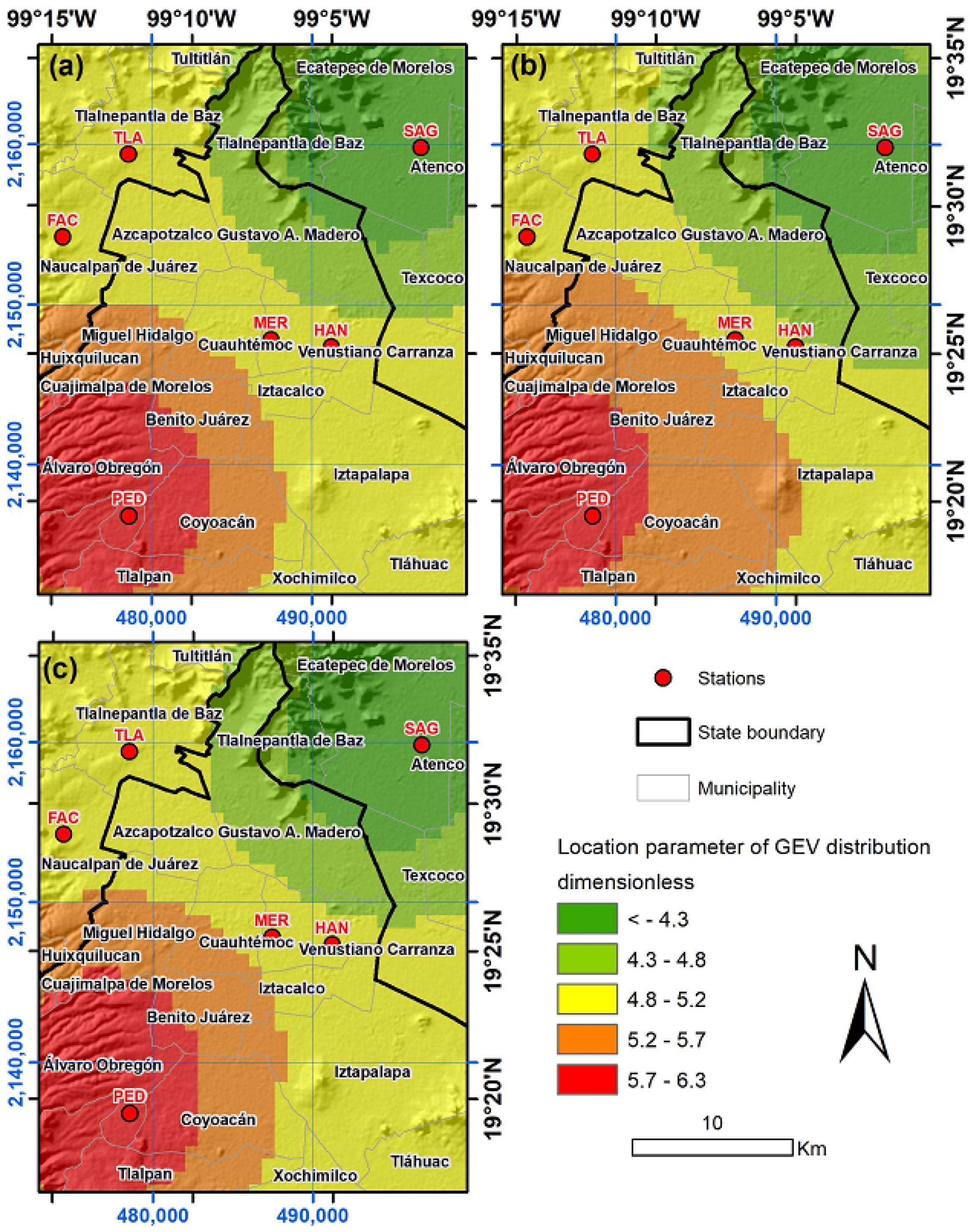
The estimates obtained for the $\sigma$ and $\kappa$ parameters were 0.2504 and −0.0356, respectively. The spatial smoothing for the years 2000, 2005, 2010, 2015, 2018 and 2019 for the location functions are shown in Figure 5. The results show well-defined patterns related to the trend in the spatial plane. The magnitude of the UVB radiation maxima decreased as we moved toward the east direction of the study area. This region coincides with the most industrialized areas of the MCMA. Therefore, these results indicate that the air pollution covariates reduce the net amount of UVB radiation that reaches the ground surface. In contrast, we observed that in the less polluted areas of MCMA there is a greater amount of UVB radiation. However, we were able to observe that, although the general trends are maintained throughout the study period, between 2010 and 2015 there was a small decrease in the intensity of UVB radiation in the central region, which return to the initial levels in 2018 and 2019. These results show that our model allowed us to identify the complete temporal dynamics of the trend throughout the study period. This is one of the strengths of the proposed model, which allows us to identify patterns in the distribution of maximum UVB radiation, make inferences and obtain conclusions about extreme values throughout the study region over time. The results also show the advantage of using a spline model with radial-based functions to estimate trends in extreme values. The nonlinear spatial function estimates in each of the different periods through a single model show the existence of the spatial variation of UVB radiation maxima. The proposed model also has the advantage that it includes the effects of covariate interactions in the model through the use of spline functions that depend on the norm of Euclidean distance between covariates and knots. This feature of the model combined with the penalty of the parameters results in a smooth continuous surface as shown in Figure 5. Future research could include the study of other types of distances between observations.

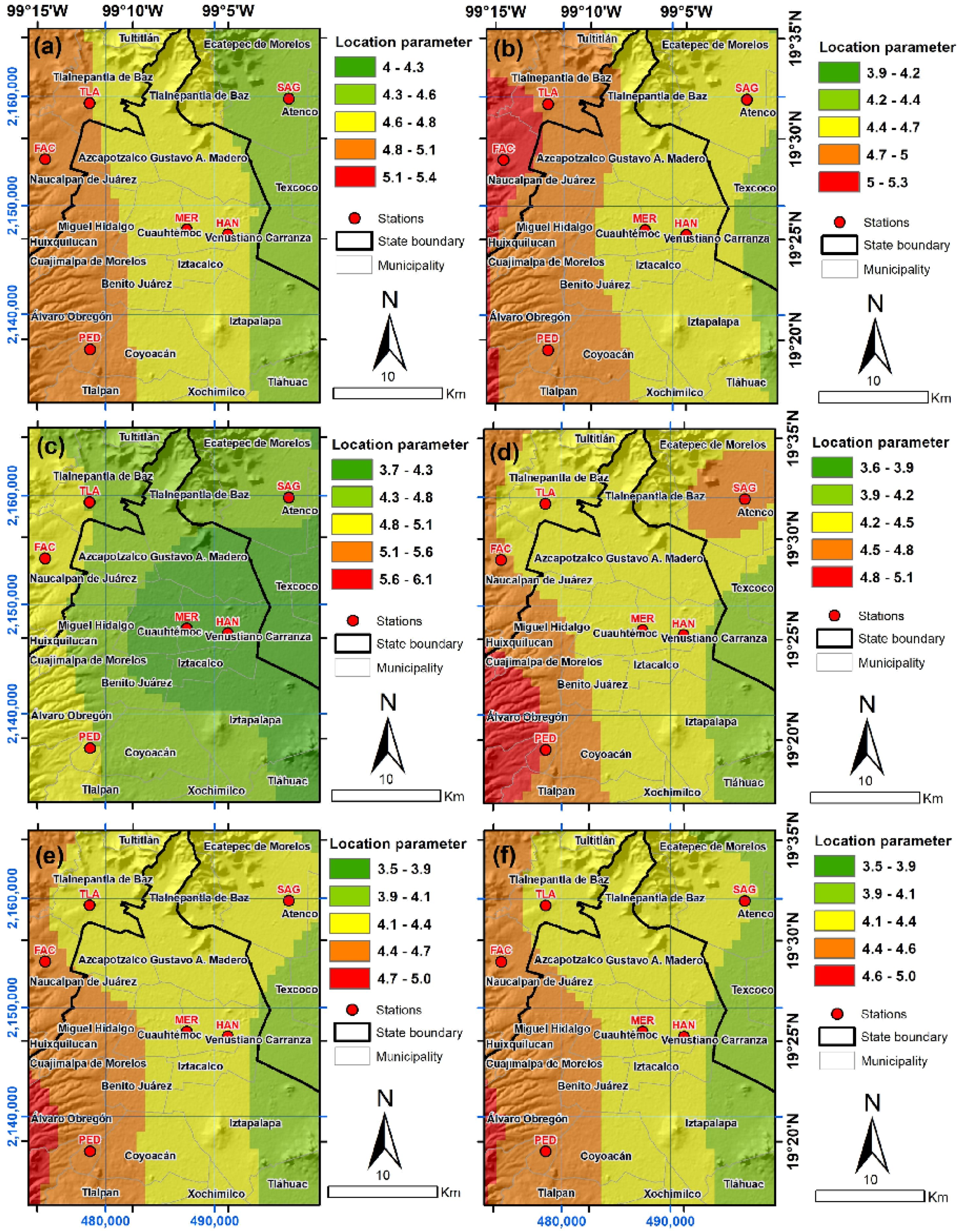
The results of the temporal trend of UVB radiation over the years keeping the other covariates constant are shown in Figure 6. In this figure, we can observe the existence of cyclic temporal patterns in the trends of the maxima in the regions located around the monitoring stations. An important finding related to the temporal behavior of the extremes, which can also be seen in Figure 6, is the decrease in the location parameter over time. An explanation for this finding could be the increase in pollution, specifically the amount of ozone (O₃), nitrogen oxides (NO_x), particles of 10 μm or less in diameter (PM₁₀) and carbon monoxide (CO), which decreases the amount of UVB radiation as a result of direct chemical reactions or by radiation blockage.

The spatial distribution of the extreme values of UVB radiation is influenced by the physicochemical interactions it has with covariates such as ozone, nitrogen oxides, particles of 10 μm or less in diameter (PM₁₀), carbon monoxide (CO), relative humidity (RH) and sulfur dioxide (SO₂) [6]. The atmospheric concentrations of some of these covariates also present seasonal behaviors which modify the intensities of UVB radiation over time. These covariates are used in the nonstationary extreme value model to estimate the trend on UVB radiation maxima, through the linear predictors corresponding to the location and scale parameters. In order to increase the likelihood of the model, we built the design matrix by using a nonlinear function of the square of distance of each observation to knots on the vector space of the observations. Each knot represented one of the k centroids resulting from a hierarchical clustering. There are several approaches to obtain a basis in the column space of the covariates, however, considering the sample size and the number of nodes, the radial basis functions are sufficient to obtain a linearly independent set.

One of the most important applications of the models obtained with the analysis of nonstationary extreme values, consists in the elaboration of risk probability maps and the return level maps. The return level $Z_p$ is the threshold at which an extreme value is exceeded with probability p, which is expected to occur once every 1/p years (Fawcett and Green [35]). Figure 7 shows the maximum expected UVB radiation for a return period of 25 years. Isolines on the map (Figure 7) were used to visualize the spatial risk of maximum UVB radiation. In fact, the highest UVB radiation values over a 25-year return period can be expected in the west part of the study area in the regions surrounding the SFE and PED monitoring stations (Figure 7). An interesting fact that explains the spatial trend of the maxima is the amount of atmospheric pollution resulted from the emissions of internal combustion vehicles and industrial emissions, among others. Further, in densely populated areas, such as the Merced or Hangares, where a large number of vehicles circulate daily, as well as in industrialized areas such as Naucalpan and Tlalnepantla, we can expect to have the lowest return levels of UVB radiation of the entire study area. An opposite situation occurs in regions farther from urban areas, in which an increase in the estimates of UVB radiation intensity can be observed. Therefore, the map of return levels shown in Figure 7 allows us to confirm the potential risk of dangerous levels of UVB radiation in the study region. These findings should encourage the creation of policies and the revision of standards related to the protection against UVB radiation as well as the delimitation of critical areas of risk.

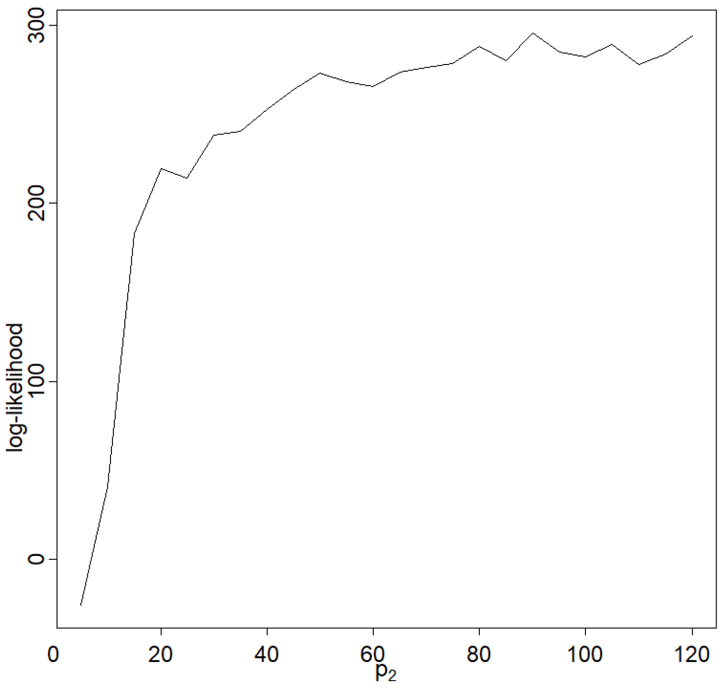
We agree with the results of Ailliot et al. [36], who reported that for stationary case, the imposing constraints improves the performance of the estimation on $\kappa$ parameter. However, we verified these results in the nonstationary case. Similar to the results of Martins and Stedinger [19], we obtained implausibly large estimates of $\kappa$ for unconstrained maximum likelihood. We observed that the Newton–Raphson method does not reach the global optimal solution for most of the initial values. This happens because we have enough variables to estimate and the quadratic approximation, which is the basis of the optimization algorithm, is not appropriate to approximate the log likelihood function when the initial values are distant from the optimal value. On this case, the optimization of the penalized log likelihood was carried out in two stages. The first stage consists of finding an initial point or seed, which will be used in the second stage of the algorithm. To achieve this, the optimization was performed in a smaller parametric space. Once the maximum is found in a parametric space with a dimension smaller than the original, we used these values as seeds or initial values to perform the approximation using the Newton–Raphson algorithm in the initial parametric space. We also agree with the results of Coles and Dixon [37], which found that estimators are improved using the maximum penalized likelihood method by restricting the range of $\kappa$.

Similar to the work of Bais et al. [38], we conclude that there is a relationship between UVB radiation and ozone, SO₂ and clouds on the spatial UVB radiation distribution across the metropolitan area of Mexico City. Other researchers have found similar relationships through direct chemical studies, concluding that chemical reactions that involve UVB radiation to produce compounds such as ozone, nitric oxide or sulfur dioxide decrease the amount of UVB radiation that reaches the ground [3,39]. There also exists other factors that interact with UVB radiation. In heavily polluted regions, there are several types of particulate matter which block the UVB radiation path [38]. The goal of our study was to analyze the spatio-temporal distribution of the UVB radiation maxima, since extremes have a strong impact on public health, while in most studies only study continuous measurements. We take advantage of the chemical interactions between air pollution and UVB radiation to model the temporal dynamics on the spatial distribution of maximas in the study area.

The monitoring and analysis of UVB radiation levels is a priority concern in terms of public health for all the largest population centers. In previous studies on UVB radiation in the metropolitan area of Mexico City, Acosta and Evans [40] found that UVB radiation levels, measured over the international standard units, reached dangerous levels for humans. We agree with their findings, in which they also detected a strong attenuation of UVB radiation at ground level in the urban troposphere under polluted conditions. However, in contrast to them, we have used the GEV distribution. An alternative to this distribution is the skew generalized extreme value distribution (SGEV) [41], which showed that it improves the return level estimation in the case of a slow convergence or in the heavy-tailed case. Future work should consider the use of the SGEV distribution for analysis of UVB radiation extremes.

4. Conclusions

In this study, we have developed a nonstationary extreme value model for UVB radiation maxima on the metropolitan area of Mexico City using a semi-parameterized model to obtain a spatio-temporal smoothing of the location parameter of the GEV distribution. We have estimated return levels of extreme events of UVB radiation through a nonstationary extreme value model in which we use both spatial and environmental covariates. UVB maxima were obtained in each of the monitoring stations through the block maxima method. The spatial and temporal trend was approximated by means of the location parameter of the GEV distribution using linear predictors based on Gaussian basis functions of the observations to knots, in order to include the effect of the interaction between the covariates in the model. One of the advantages of this model is that the estimated smooth curve allows for the adjustment of a wide variety of nonlinear functions, allowing its application in a wide variety of real situations. The regularization of the model is obtained by penalizing the parameters via penalized maximum likelihood (PML) which has the advantage of producing a shrinkage of the coefficient estimates and reducing overfitting. These methods are equivalent to the optimization of the constrained maximum likelihood and also to Bayesian methods in which the coefficients have a priori normal distributions with zero mean. The deviance test was used to validate the fitted model. The results showed that the adjusted model was significantly better than the stationary model with a reliability of 99%.

Regarding the empirical analysis of UVB radiation on the metropolitan area of Mexico City, we characterized the distribution of maxima in the spatial and temporal plane. In the spatial plane, although the results show the existence of differentiated local patterns, the estimates of the location parameter of the GEV distribution showed that there is a plane that determines the trend in the entire study region, which evidences the existence of a positive linear correlation in the west direction of the study area. These results are consistent with the demographic characteristics of the area. In the temporal plane, we observe cyclical observations on the location parameter of the spatial distribution of maxima. Such oscillations are dominated by a negative linear trend with respect to time, which is consistent with the increase in population and its corresponding consequences on air pollution. Our findings also revealed the existence of areas with well-defined spatio-temporal patterns which should help administrative authorities to improve prevention policies and standards to mitigate the impact of UVB radiation maxima. Regarding the simulation results, these demonstrate that it is feasible to identify the nonlinear characteristics of the trends reliably under the parametric conditions used in the simulation, which were established with values of the GEV parameters similar to those found in real conditions. Particularly, the spatial function for the location parameter used in the simulation, which contains nonlinear features that we can expect to find in real data, was satisfactorily estimated. However, we conclude that optimal simulations related to the distribution of nonstationary GEV is an issue that requires further investigation.

Future work can first include to analyze new functions of distance between vectors, since it is natural to think that some variables may be more important as explanatory variables than others. Secondly, to examine the asymptotic properties of the estimators regarding to the number of knots. Finally, some other further studies could consider the analysis of the sensitivity of estimates on more complex nonlinear functions using simulations on the GEV distribution under different sample sizes.

References

1. Cañada, J.; Esteve, A.; Marin, M.; Utrillas, M.; Tena, F.; Martínez-Lozano, J. Study of erythemal, UV (A+ B) and global solar radiation in Valencia (Spain). Int. J. Climatol. 2008, 28, 693–702. [Google Scholar] [CrossRef]
2. Guy, G.P., Jr.; Machlin, S.R.; Ekwueme, D.U.; Yabroff, K.R. Prevalence and Costs of Skin Cancer Treatment in the US, 2002-2006 and 2007-2011. Am. J. Prev. Med. 2015, 48, 183–187. [Google Scholar] [CrossRef] [PubMed]
3. Brönnimann, S.; Voigt, S.; Wanner, H. The influence of changing UVB radiation in near-surface ozone time series. J. Geophys. Res. Atmos. 2000, 105, 8901–8913. [Google Scholar] [CrossRef]
4. Herman, J.R. Global increases in UVB irradiance from changes in ozone and cloud-aerosol amounts 1979 to 2008. Proc. SPIE 2009, 7462, 746206. [Google Scholar]
5. Langston, M.; Dennis, L.; Lynch, C.; Roe, D.; Brown, H. Temporal trends in satellite-derived Erythemal UVB and implications for ambient Sun exposure assessment. Int. J. Environ. Res. Public. Health 2017, 14, 176. [Google Scholar] [CrossRef] [PubMed] [Green Version]
6. Valdés-Barrón, M.; Bonifaz-Alfonzo, R.; Riveros-Rosas, D.; Velasco-Herreora, V.; Estévez-Pérez, H.; Peláez-Chávez, J.C. UVB solar radiation climatology for Mexico. Geofis. Int. 2013, 52, 31–42. [Google Scholar] [CrossRef] [Green Version]
7. Sun, Y.; Song, T.; Tang, G.; Wang, Y. The vertical distribution of PM2. 5 and boundary-layer structure during summer haze in Beijing. Atmos. Environ. 2013, 74, 413–421. [Google Scholar] [CrossRef]
8. McKenzie, R.; Weinreis, C.; Johnston, P.; Liley, B.; Shiona, H.; Kotkamp, M.; Smale, D.; Takegawa, N.; Kondo, Y. Effects of urban pollution on UV spectral irradiances. Atmos. Chem. Phys. Discuss. 2008, 8, 7149–7188. [Google Scholar] [CrossRef]
9. Fisher, R.A.; Tippett, L.H.C. Limiting forms of the frequency distribution of the largest or smallest member of a sample. Proc. Camb. Philos. Soc. 1928, 24, 180–190. [Google Scholar] [CrossRef]
10. Gnedenko, B.V. On a local limit theorem of the theory of probability. Uspekhi Matematicheskikh Nauk 1948, 3, 187–194. [Google Scholar]
11. Jenkinson, A.F. The frequency distribution of the annual maximum (or minimum) values of meteorological elements. Quart. J. Roy. Meteor. Soc. 1955, 81, 158–171. [Google Scholar] [CrossRef]
12. Prescott, P.; Walden, A. Maximum likeiihood estimation of the parameters of the three-parameter generalized extreme-value distribution from censored samples. J. Stat. Comput. Simul. 1983, 16, 241–250. [Google Scholar] [CrossRef]
13. Phien, H.N.; Fang, T.S.E. Maximum likelihood estimation of the parameters and quantiles of the general extreme-value distribution from censored samples. J. Hydrol. 1989, 105, 139–155. [Google Scholar] [CrossRef]
14. Wang, Q. Using partial probability weighted moments to fit the extreme value distributions to censored samples. Water Resour. Res. 1996, 32, 1767–1771. [Google Scholar] [CrossRef]
15. Gaetan, C.; Grigoletto, M. A hierarchical model for the analysis of spatial rainfall extremes. J. Agric. Biol. Environ. Stat. 2007, 12, 434–449. [Google Scholar] [CrossRef]
16. Reich, B.; Shaby, B.; Cooley, D. A Hierarchical Model for Serially-Dependent Extremes: A Study of Heat Waves in the Western US. J. Agric. Biol. Environ. Stat. 2014, 19, 119–135. [Google Scholar] [CrossRef]
17. Bhattarai, K.P. Partial L-moments for the analysis of censored flood samples/Utilisation des L-moments partiels pour lánalyse d’échantillons tronqués de crues. Hydrol. Sci. J. 2004, 49, 868. [Google Scholar] [CrossRef] [Green Version]
18. Hosking, J.R. L-moments: Analysis and estimation of distributions using linear combinations of order statistics. J. R. Stat. Soc. Ser. B 1990, 52, 105–124. [Google Scholar] [CrossRef]
19. Martins, E.; Stedinger, J. Generalized maximum-likelihood generalized extreme-value quantile estimators for hydrologic data. Water Resour. Res. 2000, 36, 737–744. [Google Scholar] [CrossRef]
20. Coles, S. An Introduction to Statistical Modeling of Extreme Values; Springer: Berlin/Heidelberg, Germany, 2001; Volume 208. [Google Scholar]
21. Bocci, C.; Caporali, E.; Petrucci, A. Geoadditive modeling for extreme rainfall data. AStA Adv. Stat. Anal. 2013, 97, 181–193. [Google Scholar] [CrossRef]
22. Dupuis, D.; Field, C. Large wind speeds: Modeling and outlier detection. J. Agric. Biol. Environ. Stat. 2004, 9, 105. [Google Scholar] [CrossRef]
23. Nordquist, J.M. Theory of largest values applied to earthquake magnitudes. Eos Trans. Am. Geophys. Union 1945, 26, 29–31. [Google Scholar] [CrossRef]
24. Makjanić, B. On the frequency distribution of earthquake magnitude and intensity. Bull. Seismol. Soc. Am. 1980, 70, 2253–2260. [Google Scholar]
25. Weissman, I. Estimation of parameters and large quantiles based on the k largest observations. J. Am. Stat. Assoc. 1978, 73, 812–815. [Google Scholar]
26. Tawn, J. Bivariate extreme value theory: Models and estimation. Biometrika 1988, 75, 397–415. [Google Scholar] [CrossRef]
27. Pauli, F.; Coles, S. Penalized likelihood inference in extreme value analyses. J. Appl. Stat 2001, 28, 547–560. [Google Scholar] [CrossRef]
28. Yee, T.W.; Stephenson, A.G. Vector generalized linear and additive extreme value models. Extremes 2007, 10, 1–19. [Google Scholar] [CrossRef]
29. Rodríguez, S.; Reyes, H.; Pérez, P.; Vaquera, H. Selection of a subset of meteorological variables for ozone analysis: Case study of pedregal station in Mexico City. Environ. Sci. Eng. A. 2012, 1, 11–20. [Google Scholar]
30. Cannon, A.J. A flexible nonlinear modelling framework for nonstationary generalized extreme value analysis in hydroclimatology. Hydrol. Process. 2010, 24, 673–685. [Google Scholar] [CrossRef]
31. Sang, H.; Gelfand, A.E. Continuous spatial process models for spatial extreme values. J. Agric. Biol. Environ. Stat. 2010, 15, 49–65. [Google Scholar] [CrossRef]
32. Figueiredo, M.A. On Gaussian radial basis function approximations: Interpretation, extensions, and learning strategies. In Proceedings of the 15th International Conference on Pattern Recognition (ICPR-2000), Barcelona, Spain, 3–7 September 2000; Volume 2, pp. 618–621. [Google Scholar]
33. Ross, S.M. Simulation, 4th ed.; Academic Press, Inc.: Cambridge, MA, USA, 2006. [Google Scholar]
34. R Core Team. R: A Language and Environment for Statistical Computing; R Foundation for Statistical Computing: Vienna, Austria, 2017. [Google Scholar]
35. Fawcett, L.; Green, A.C. Bayesian posterior predictive return levels for environmental extremes. Stoch. Environ. Res. Risk. Assess. 2018, 32, 2233–2252. [Google Scholar] [CrossRef] [Green Version]
36. Ailliot, P.; Thompson, C.; Thomson, P. Mixed methods for fitting the GEV distribution. Water Resour. Res. 2011, 47. [Google Scholar] [CrossRef]
37. Coles, S.G.; Dixon, M.J. Likelihood-based inference for extreme value models. Extremes 1999, 2, 5–23. [Google Scholar] [CrossRef]
38. Bais, A.F.; Zerefos, C.S.; Meleti, C.; Ziomas, I.C.; Tourpali, K. Spectral measurements of solar UVB radiation and its relations to total ozone, SO2, and clouds. J. Geophys. Res. Atmos. 1993, 98, 5199–5204. [Google Scholar] [CrossRef]
39. Kleinman, L.I. Low and high NOx tropospheric photochemistry. J. Geophys. Res. Atmos. 1994, 99, 16831–16838. [Google Scholar] [CrossRef]
40. Acosta, L.; Evans, W. Design of the Mexico City UV monitoring network: UV-B measurements at ground level in the urban environment. J. Geophys. Res. Atmos. 2000, 105, 5017–5026. [Google Scholar] [CrossRef]
41. Ribereau, P.; Masiello, E.; Naveau, P. Skew generalized extreme value distribution: Probability-weighted moments estimation and application to block maxima procedure. Commun. Stat-Theor. M. 2016, 45, 5037–5052. [Google Scholar] [CrossRef]
Figure 1. Study area.
Mathematics 08 00329 g001
Figure 2. Log-likelihood function averaged over fifty independent simulations at each value of p 2 .
Mathematics 08 00329 g002
Figure 3. (a) Real functions, (b) and (c) are functions obtained by fitting the parameters of a nonstationary generalized extreme value (GEV) model with P 2 = 10 and P 2 = 80 knots respectively, to simulated data with a sample size of n = 500 .
Mathematics 08 00329 g003
Figure 4. Boxplots of the ultraviolet B radiation (UVB) maxima at seven monitoring stations in the Mexico City metropolitan area.
Mathematics 08 00329 g004
Figure 5. Estimated spatial smoothing of the location parameter for the years (a) 2000, (b) 2005, (c) 2010, (d) 2015, (e) 2018 and (f) 2019.
Mathematics 08 00329 g005
Figure 6. Estimates of the temporal trend for the location GEV parameter of the UVB radiation maxima distribution for monitoring station.
Mathematics 08 00329 g006
Figure 7. Spatial distribution of 25-year return period extreme UVB radiation estimation in North Mexico City.
Mathematics 08 00329 g007