Responsive Economic Model Predictive Control for Next-Generation Manufacturing

Abstract

There is an increasing push to make automated systems capable of carrying out tasks which humans perform, such as driving, speech recognition, and anomaly detection. Automated systems, therefore, are increasingly required to respond to unexpected conditions. Two types of unexpected conditions of relevance in the chemical process industries are anomalous conditions and the responses of operators and engineers to controller behavior. Enhancing responsiveness of an advanced control design known as economic model predictive control (EMPC) (which uses predictions of future process behavior to determine an economically optimal manner in which to operate a process) to unexpected conditions of these types would advance the move toward artificial intelligence properties for this controller beyond those which it has today and would provide new thoughts on interpretability and verification for the controller. This work provides theoretical studies which relate nonlinear systems considerations for EMPC to these higher-level concepts using two ideas for EMPC formulations motivated by specific situations related to self-modification of a control design after human perceptions of the process response are received and to controller handling of anomalies.

1. Introduction

The buzz around artificial intelligence (AI), machine learning, and data in recent years has sparked both excitement and skepticism from the process systems engineering community [1,2]. Some of the most prevalent uses of data in the process systems field have included its use in developing models of various processes (e.g., Reference [3]) with potential applications in model-based control [4], in learning control laws [5,6], and in process monitoring [7,8]. Control engineers have debated about whether control itself should be considered to be artificial intelligence, particularly as control laws become more advanced. For example, a particularly intelligent form of control (known as economic model predictive control (EMPC) [9,10,11,12]) is an optimization-based control strategy that determines the optimal manner in which to operate a chemical process in the sense that the control actions optimize a profit metric for the process over a prediction horizon, subject to process constraints. The significant potential benefits of this control law for next-generation manufacturing have prompted a wide range of investigations in the context of EMPC, including how it may be used for building temperature regulation [13], wastewater treatment [14], microgrid dispatch [15], and gas pipeline networks [16]. Though chemical processes have traditionally been operated at steady-state, EMPC does not necessarily enforce steady-state operation in its efforts to optimize process economic performance. This has raised key questions for this control design regarding important properties of intelligent systems such as interpretability of its operating strategy and verification that it will work correctly for the real environment that it will need to control and interact with.

Interpretability is a desirable property for artificially intelligent systems. It has been considered in a variety of contexts; for example, the issue of building interpretable data-driven models has been considered to be enhanced by sparse regression, where a model with a small number of available possible terms which could be utilized to build it is derived (with an underlying assumption being that simpler models are more physically realistic and therefore should be more interpretable) [17]. Models identified via sparse regression techniques have been utilized in model predictive control for hydraulic fracturing [18]. Interpretability of other model-building strategies has also been a consideration; for example, for neural networks, where interpretability may be considered to be multidimensional, but to generally constitute whether a human can trace how a neural network obtained its conclusions via how the input information was processed [19], recurrent neural networks with long short-term memory were analyzed for how their cells processed different aspects of character-level language models [20].

It is recognized that interpretability of the control actions computed by an EMPC will be a major determining factor in the adoption of EMPC in the process industries (because, if operators and engineers do not know if the process is in an upset condition, they will likely disable features of the controller that make it difficult to understand due to the need to be sure that safety is maintained at all times). Interpretability for EMPC has not yet received significant focus in the literature. The subset of EMPC formulations which track a steady-state [21] possess a form of interpretability in that the reference behavior is understood by engineers and operators. Reference [22] developed an EMPC formulation in which the desired closed-loop process response specified or restricted by an operator or engineer is tracked by the controller. However, developing the best means for ensuring interpretability for EMPC to appropriately trade off end user understanding with economic optimality remains a largely open question. This work provides new perspectives on this important issue, suggesting that a controller formulation that bridges the human–machine interface by allowing the adjustment of constraints in response to human opinions about the process behavior under the EMPC may provide new avenues of both democratizing advanced control and allowing end users to adjust the response to their liking from an interpretability standpoint.

Another important topic for intelligent control systems is enabling their verification (i.e., certifying that they will perform in practice as intended). Verification can take a significant amount of engineering time and expense, and methods for reducing the time required to validate the controller’s performance could reduce the cost of advanced control, could promote operational safety, and could make the controller more straightforward to implement (a lack of ability to verify can prevent an intelligent system from being placed online at all). In the control community, a traditional approach to verification is to design controllers with guaranteed robustness to bounded uncertainty and to use this as a certificate that the controller will be able to maintain closed-loop stability in practice (e.g., References [23,24,25]). This requires some knowledge of the disturbance characteristics (e.g., upper bounds), which may be difficult to fully determine a priori but is important for EMPC, as the controller could drive the closed-loop state to operate at boundaries of safe operating regions to optimize profits, where the uncertainty in the disturbance characteristics could lead to unsafe conditions. Additional conservatism to account for the uncertainty could lead to over-conservatism that could decrease profits. Other methods for handling disturbances in EMPC have been developed, including methods that account for disturbances probabilistically (making assumptions on their distribution) [26] or adapting models used by the predictive controller online (e.g., References [27,28,29]). Results on the use of adapting models in EMPC have even included closed-loop stability guarantees when a recurrent neural network that is updated via error triggering is used as the process model [30]. An example of an adaptive control strategy which handles uncertain dynamics in batch processing is that in Reference [31], which uses model predictive control equipped with a probabilistic recursive least squares model parameter update algorithm with a forgetting factor to capture batch process dynamics. In addition, Reference [32] analyzed a learning-based MPC strategy with a terminal constraint for systems with unmodeled dynamics, where performance is enhanced by using a learned model in the MPC but safety goals are met by ensuring that control actions computed via the MPC are stabilizing.

Another direction that has received attention for handling uncertainty is fault tolerance in the sense of controller reconfigurations upon detection of an actuator fault/anomaly (e.g., Reference [33]) or anomaly response cast in a framework of fault-tolerant control handled via fault/anomaly detection followed by updating the model used by a model-based controller [34]. In Reference [35], fault-tolerant control for nonlinear switched systems was analyzed in the context of safe parking for model predictive control with a steady-state tracking objective function for actuator faults. For EMPC, Reference [36] handled faults through error-triggered data-driven model updates in the controller, and the uniting of EMPC with driving the state into safety-based regions in state-space (e.g., References [37,38]) also constitutes a form of fault-handling. Despite these advances in handling anomalies and uncertainty, which are critical for addressing moving toward a verification paradigm for EMPC, verifying the controller today would still be expected to be time-consuming; additional work is needed to explore further ways of considering and establishing verification for the control design.

Another approach in verification of controllers has been online verification via data-driven models complemented by detection algorithms for problematic controller behavior leading to bounds on the time that would elapse before detection of problematic controller behavior [39]. A feature of this direction in verification, therefore, is the combination of data-driven modeling for control (to address model uncertainty) with guarantees that problematic behavior due to model inaccuracies can be flagged within a given time period. In the present work, we take a conceptually similar approach to verification for EMPC using online anomaly handling with a conservative Lyapunov-based EMPC (LEMPC) [24] design approach that facilitates guaranteed detection of significant plant/model mismatch under sufficient conditions and allows upper bounds on the amount of time available until the mismatch would need to be compensated via model updates without compromising closed-loop stability (as well as the characteristics of the resulting control law after model reidentification required to obtain these theoretical results) to be presented. The development of theoretical guarantees on closed-loop stability with data-driven models that can be updated online in LEMPC has some similarities to References [30,40] but is pursued from a different angle that allows the underlying process dynamics to suddenly change and also allows for more general nonlinear data-driven models to be considered (i.e., we do not restrict the modeling methodology to neural networks as in References [30,40]). It also has similarities to the framework for accounting for faults in LEMPC via model updates in Reference [41] but considers a theoretical treatment of anomaly conditions with data-driven LEMPC, which was not explored in that work.

Motivated by the above considerations, this work focuses on advancing both interpretability and verification for EMPC. These are important considerations for human–machine interaction and can be viewed as different aspects of a “responsive” control design in the sense that the controller is made responsive to changing or unexpected conditions like a human would be. We first address the interpretability concept suggested above in an LEMPC framework in which we elucidate conditions under which an LEMPC could be made responsive to potentially inaccurate metrics reflecting the reactions of end users to the LEMPC’s behavior without loss of closed-loop stability. We subsequently move in the direction of addressing verification considerations for LEMPC by developing theoretical guarantees which can be made for the controller in the presence of process dynamics anomalies/changes when potentially adapting data-driven models are used in the controller. We evaluate the conditions under which closed-loop stability may be lost in such circumstances, with exploration of bounds on times before which detection and accommodation of the anomaly could be stabilized to avoid potential plant shutdown. Numerical examples utilizing continuous stirred tank reactors (CSTRs) are presented to illustrate major concepts. Throughout, we highlight cases where the proposed methods could interface with other artificial intelligence techniques (e.g., sentiment analysis or image-based sensing) without compromising closed-loop stability, highlighting the range of intelligent techniques which can be used to enhance next-generation control within an appropriate theoretical framework.

This work is organized as follows: in Section 2, preliminaries are presented. These are followed by the main results in Section 3, which consist of controller formulations and implementation strategies, with demonstration via numerical examples, where (1) the controller constraints can be adjusted online in response to potentially inaccurate stimuli without closed-loop stability being lost (Section 3.1) and (2) the control strategy has characterizable properties in the presence of process anomalies resulting in unanticipated changes in the underlying process dynamics (Section 3.2). Section 4 concludes and provides an outlook on the presented results. Proofs for theoretical results associated with the second control strategy noted above are provided in the Appendix. This manuscript is an extended version of Reference [42].

2. Preliminaries

2.1. Notation

The operator $|·|$ denotes the vector Euclidean norm. A function $\alpha :[0,a)\to [0,\infty )$ is in class $\mathcal{K}$ if it is continuous, if it strictly increases, and if $\alpha (0)=0$. The notation ${\mathsf{\Omega }}_{\rho }$ defines a level set of a scalar-valued function V (i.e., ${\mathsf{\Omega }}_{\rho }:=\{x\in R^n : V(x)\le \rho \}$). The operator ${}^{\prime }{/}^{\prime }$ signifies set subtraction (i.e., $A/B:=\{x\in R^n : x\in A, x\notin B\}$). $x^T$ represents the transpose of the vector x. We define a sampling time with the notation $t_k:=k\Delta$, $k=0,1,\dots$.

2.2. Class of Systems

This work considers switched nonlinear systems of the following form:

$${\dot{x}}_{a,i}=f_i(x_{a,i}(t),u(t),w_i(t))$$

(1)

where $x_{a,i}\in X\subset R^n$ denotes the state vector, $u\in U\subset R^m$ denotes the input vector ($u={[u_1,\dots ,u_m]}^T$), and $w_i\in W_i\subset R^z$ denotes the disturbance vector, where $W_i:=\{w_i\in R^z : |w_i|\le {\theta }_i, {\theta }_i>0\}$, for $i=1,2,\dots$. In this notation, the ith model is used for $t\in [t_{s,i},t_{s,i+1})$, where $x_{a,i}(t_{s,i+1})=x_{a,i+1}(t_{s,i+1})$ and $t_{s,1}=t_0$. The vector function $f_i$ is assumed to be a locally Lipschitz function of its arguments with $f_1(0,0,0)=0$ and $f_i(x_{a,i,s},u_{i,s},0)=0$ for $i>1$ (i.e., the steady-state of the updated models when $w_i=0$ is at $x_{a,i}=x_{a,i,s}$, $u=u_{i,s}$). The system of Equation (1) with $w_i\equiv 0$ is known as the nominal system. Synchronous measurement sampling is assumed, with measurements available at every $t_k=k\Delta$, $k=0,1,\dots$. It is noted that $t_{s,i}$, $i=1,2,\dots$, is not required to be an integer multiple of $t_k$. We define ${\overline{x}}_{a,i}=x_{a,i}-x_{a,i,s}$ and ${\overline{u}}_i=u-u_{i,s}$ and define ${\overline{f}}_i$ as $f_i$ rewritten to have its origin at ${\overline{x}}_{a,i}=0$, ${\overline{u}}_i=0$, $w_i=0$. Similarly, we define $U_i$ to be the set U in deviation variable form from $u_{i,s}$ and $X_i$ to be the set X in deviation variable form from $x_{a,i,s}$.

We assume that there exists an explicit stabilizing (Lyapunov-based) control law $h_i({\overline{x}}_{a,i})={[h_{i,1}({\overline{x}}_{a,i}) \dots h_{i,m}({\overline{x}}_{a,i})]}^T$ that renders the origin of the nominal system of Equation (1) asymptotically stable in the sense that the following inequalities hold:

$${\alpha }_{1,i}(|{\overline{x}}_{a,i}|)\le V_i({\overline{x}}_{a,i})\le {\alpha }_{2,i}(|{\overline{x}}_{a,i}|)$$

(2)

$$\frac{\partial V_i({\overline{x}}_{a,i})}{\partial {\overline{x}}_{a,i}}{\overline{f}}_i({\overline{x}}_{a,i},h_i({\overline{x}}_{a,i}),0)\le -{\alpha }_{3,i}(|{\overline{x}}_{a,i}|)$$

(3)

$$\left|\frac{\partial V_i({\overline{x}}_{a,i})}{\partial {\overline{x}}_{a,i}}\right|\le {\alpha }_{4,i}(|{\overline{x}}_{a,i}|)$$

(4)

$$h_i({\overline{x}}_{a,i})\in U_i$$

(5)

for all ${\overline{x}}_{a,i}\in D_i\subseteq R^n$ and $i=1,2,\dots$, where $D_i$ is an open neighborhood of the origin of ${\overline{f}}_i$, and for a positive definite, sufficiently smooth Lyapunov function $V_i$. The functions ${\alpha }_{1,i}$, ${\alpha }_{2,i}$, ${\alpha }_{3,i}$, and ${\alpha }_{4,i}$ are of class $\mathcal{K}$. A level set of $V_i$ denoted by ${\mathsf{\Omega }}_{{\rho }_i}\subset D_i$ is referred to as the stability region of the system of Equation (1) under the controller $h_i({\overline{x}}_{a,i})$. We consider that ${\mathsf{\Omega }}_{{\rho }_i}$ is selected to be contained within X. The Lyapunov-based controller is assumed to be Lipschitz continuous such that the following inequalities hold:

$$|h_{i,j}(x)-h_{i,j}(x^{\prime })|\le L_{h,i}|x-x^{\prime }|$$

(6)

for a positive constant $L_{h,i}$ for all $x,x^{\prime }\in {\mathsf{\Omega }}_{{\rho }_i}$, and $i=1,2,\dots$, with $j=1,\dots ,m$.

Lipschitz continuity of $f_i$ and sufficient smoothness of $V_i$ provide the following inequalities, for positive constants $M_i$, $L_{x,i}$, $L_{w,i}$, $L_{x,i}^{\prime }$, and $L_{w,i}^{\prime }$:

$$|{\overline{f}}_i(x,u,w_i)|\le M_i$$

(7)

$$|{\overline{f}}_i(x,u,w_i)-{\overline{f}}_i(x^{\prime },u,0)|\le L_{x,i}|x-x^{\prime }|+L_{w,i}\left|w_i\right|$$

(8)

$$\left|\frac{\partial V_i(x)}{\partial x}{\overline{f}}_i(x,u,w_i)-\frac{\partial V_i(x^{\prime })}{\partial x}{\overline{f}}_i(x^{\prime },u,0)\right|\le L_{x,i}^{\prime }|x-x^{\prime }|+L_{w,i}^{\prime }\left|w_i\right|$$

(9)

for all $x,x^{\prime }\in {\mathsf{\Omega }}_{{\rho }_i}$, $u\in U_i$, and $w_i\in W_i$.

As this work considers responses to unexpected conditions, we consider that there may be cases in which the nonlinear model of Equation (1) may not be available, though an empirical model with the following form may be available:

$$\begin{array}{c}\hfill {\dot{x}}_{b,q}(t)=f_{NL,q}(x_{b,q}(t),u(t))\end{array}$$

(10)

where $f_{NL,q}$ is a locally Lipschitz nonlinear vector function in $x_{b,q}\in {\mathbb{R}}^n$ and in the input $u\in {\mathbb{R}}^m$ with $f_{NL,1}(0,0)=0$ and $f_{NL,q}(x_{b,q,s},u_{q,s})=0$ for $q>1$ (i.e., the steady-state of the updated models is at $x_{b,q}=x_{b,q,s}$, $u=u_{q,s}$). Here, $q=1,2,\dots$, to allow for the possibility that, as the underlying process dynamics change (i.e., the value of i increases in Equation (1)), it may be desirable to switch the empirical model used to describe the system. However, we utilize the index q instead of i for the empirical model to signify that we do not assume that the empirical model must switch with the same frequency as the process dynamics. When the model of Equation (10) does switch, we assume that the switch occurs at a time $t_{s,NL,q+1}$ in a manner where $x_{b,q}(t_{s,NL,q+1})=x_{b,q+1}(t_{s,NL,q+1})$. We define ${\overline{x}}_{b,q}=x_{b,q}-x_{b,q,s}$ and ${\overline{u}}_q=u-u_{q,s}$ and define ${\overline{f}}_{NL,q}$ as $f_{NL,q}$, rewritten to have its origin at ${\overline{x}}_{b,q}=0$, ${\overline{u}}_q=0$, as follows:

$$\begin{array}{c}\hfill {\dot{\overline{x}}}_{b,q}(t)={\overline{f}}_{NL,q}({\overline{x}}_{b,q}(t),{\overline{u}}_q(t))\end{array}$$

(11)

Similarly, we define $U_q$ to be the set U in deviation variable form from $u_{q,s}$ and $X_q$ to be the set X in deviation variable form from $x_{b,q,s}$.

We consider that, for the empirical models in Equation (10), there exists a locally Lipschitz explicit stabilizing controller $h_{NL,q}({\overline{x}}_{b,q})$ that can render the origin asymptotically stable in the sense that:

$$\begin{array}{c}{\widehat{\alpha }}_{1,q}(|{\overline{x}}_{b,q}|)\le {\widehat{V}}_q({\overline{x}}_{b,q})\le {\widehat{\alpha }}_{2,q}(|{\overline{x}}_{b,q}|)\hfill \end{array}$$

(12a)

$$\begin{array}{c}\frac{\partial {\widehat{V}}_q({\overline{x}}_{b,q})}{\partial {\overline{x}}_{b,q}}{\overline{f}}_{NL,q}({\overline{x}}_{b,q},h_{NL,q}({\overline{x}}_{b,q}))\le -{\widehat{\alpha }}_{3,q}(|{\overline{x}}_{b,q}|)\hfill \end{array}$$

(12b)

$$\begin{array}{c}\left|\frac{\partial {\widehat{V}}_q({\overline{x}}_{b,q})}{\partial {\overline{x}}_{b,q}}\right|\le {\widehat{\alpha }}_{4,q}(|{\overline{x}}_{b,q}|)\hfill \end{array}$$

(12c)

$$\begin{array}{c}{h}_{NL,q}({\overline{x}}_{b,q})\in U_q\hfill \end{array}$$

(12d)

for all ${\overline{x}}_{b,q}\in D_{NL,q}$ (where $D_{NL,q}$ is a neighborhood of the origin of ${\overline{f}}_{b,q}$ contained in X), where ${\widehat{V}}_q:{\mathbb{R}}^n\to {\mathbb{R}}_{+}$ is a sufficiently smooth Lyapunov function, ${\widehat{\alpha }}_{i,q},i=1,2,3,4,$ are class $\mathcal{K}$ functions, and $q=1,2,\dots$. We define ${\mathsf{\Omega }}_{{\widehat{\rho }}_q}\subset D_{NL,q}$ as the stability region of the system of Equation (10) under $h_{NL,q}$ and ${\mathsf{\Omega }}_{{\widehat{\rho }}_{safe,q}}$ as a superset of ${\mathsf{\Omega }}_{{\widehat{\rho }}_q}$ contained in $D_{NL,q}$ and X. Lipschitz continuity of $f_{NL,q}$ and sufficient smoothness of ${\widehat{V}}_q$ imply that there exist $M_{L,q}>0$ and $L_{L,q}>0$ such that

$$\begin{array}{c}|{\overline{f}}_{NL,q}(x,u)|\le M_{L,q}\hfill \end{array}$$

(13a)

$$\begin{array}{c}|\frac{\partial {\widehat{V}}_q(x_1)}{\partial x}{\overline{f}}_{NL,q}(x_1,u)-\frac{\partial {\widehat{V}}_q(x_2)}{\partial x}{\overline{f}}_{NL,q}(x_2,u)|\le L_{L,q}|x_1-x_2|\hfill \end{array}$$

(13b)

$\forall x,x_1,x_2\in {\mathsf{\Omega }}_{{\widehat{\rho }}_q}$, $u\in U_q$, and $q=1,2,\dots$.

Furthermore, we define ${\overline{x}}_{a,i,q}=x_{a,i}-x_{b,q,s}$ as the variable representing the deviation of each $x_{a,i}$ from the steady-state of the qth empirical model of Equation (10) and ${\overline{f}}_{i,q}$ as the right-hand side of Equation (1) when the model is rewritten in terms of the deviation variables ${\overline{x}}_{a,i,q}$ and ${\overline{u}}_q$, as follows:

$${\dot{\overline{x}}}_{a,i,q}={\overline{f}}_{i,q}({\overline{x}}_{a,i,q}(t),{\overline{u}}_q(t),w_i(t))$$

(14)

We assume that the following holds:

$$|{\overline{f}}_{i,q}(x,u^{\prime },w)-{\overline{f}}_{i,q}(x^{\prime },u^{\prime },0)|\le L_{x,i,q}|x-x^{\prime }|+L_{w,i,q}\left|w\right|$$

(15)

$$\left|\frac{\partial {\widehat{V}}_q(x)}{\partial x}{\overline{f}}_{i,q}(x,u^{\prime },w)-\frac{\partial {\widehat{V}}_q(x^{\prime })}{\partial x}{\overline{f}}_{i,q}(x^{\prime },u^{″},0)\right|\le L_{x,i,q}^{\prime }|x-x^{\prime }|+L_{w,i,q}^{\prime }\left|w\right|$$

(16)

for all $x,x^{\prime },u^{\prime },u^{″}$ and w such that $x+x_{b,q,s}-x_{a,i,s}\in {\mathsf{\Omega }}_{{\rho }_i}$, $x^{\prime }+x_{b,q,s}-x_{a,i,s}\in {\mathsf{\Omega }}_{{\rho }_i}$, $u^{\prime }+u_q\in U$, $u^{″}+u_q\in U$, and $w\in W_i$. We define a level set of ${\widehat{V}}_q$ contained in ${\mathsf{\Omega }}_{{\widehat{\rho }}_{safe,q}}$ that is also contained in ${\mathsf{\Omega }}_{{\rho }_i}$ to be ${\mathsf{\Omega }}_{{\widehat{\rho }}_{q,i}}$, and $L_{x,i,q},L_{w,i,q},L_{x,i,q}^{\prime },L_{w,i,q}^{\prime }>0$

2.3. Economic Model Predictive Control

Economic model predictive control (EMPC) [12] is an optimization-based control design formulated as follows:

$${min}_{{\overline{u}}_i\in S(\Delta )}{\int }_{t_k}^{t_{k+N}}{L}_e({\tilde{\overline{x}}}_{a,i}(\tau ),{\overline{u}}_i(\tau ))d\tau$$

(17)

$$\mathrm{s}.\mathrm{t}. {\dot{\tilde{\overline{x}}}}_{a,i}(t)={\overline{f}}_i({\tilde{\overline{x}}}_{a,i}(t),{\overline{u}}_i(t),0)$$

(18)

$${\tilde{\overline{x}}}_{a,i}(t_k)=x(t_k)$$

(19)

$${\overline{u}}_i(t)\in U_i, \forall t\in [t_k,t_{k+N})$$

(20)

$${\tilde{\overline{x}}}_{a,i}(t)\in X_i, \forall t\in [t_k,t_{k+N})$$

(21)

where $L_e(·,·)$ represents the stage cost of the EMPC, which can be a general scalar-valued function that is optimized in Equation (17). The notation $u\in S(\Delta )$ signifies that u is a piecewise-constant input trajectory with period $\Delta$. The prediction horizon is denoted by N. Equation (18) represents the nominal process model, with predicted state ${\tilde{\overline{x}}}_{a,i}$ for the ith model. Equations (20) and (21) represent the input and state constraints, respectively. We denote the optimal solution of an EMPC at $t_k$ by $u_p^{*}(t_j|t_k)$, $p=1,\dots ,m$, $j=k,\dots ,k+N-1$, where each $u_p^{*}(t_j|t_k)$ holds for $t\in [t_j,t_{j+1})$ within the prediction horizon. $x(t_k)$ in Equation (19) signifies that the state measurement represents the actual system state at $t_k$ placed in deviation variable form with respect to ${\overline{x}}_{a,i,s}$. Due to the potential switching of the underlying process dynamics before the model in Equation (18) is updated, the measurement may come from a dynamic system different than the ith model used in Equation (18).

2.4. Lyapunov-Based Economic Model Predictive Control

A variety of variations on the general EMPC formulation in Equations (17)–(21) have been developed. One such variation which will receive focus in this paper is Lyapunov-based EMPC (LEMPC) [24], which is formulated as in Equations (17)–(21) but with the following Lyapunov-based constraints added as well:

$$V_i({\tilde{\overline{x}}}_{a,i}(t))\le {\rho }_{e,i}, \forall t\in [t_k,t_{k+N}), \mathrm{if} t_k\le t^{\prime } \mathrm{and} V_i(x(t_k))\le {\rho }_{e,i}$$

(22)

$$\begin{array}{c}\frac{\partial V_i(x(t_k))}{\partial x}{\overline{f}}_i(x(t_k),u(t_k),0)\le \frac{\partial V_i(x(t_k))}{\partial x}{\overline{f}}_i(x(t_k),h_i(x(t_k)),0),\hfill \\ \mathrm{if} t_k>t^{\prime } \mathrm{or} V_i(x(t_k))>{\rho }_{e,i}\hfill \end{array}$$

(23)

where ${\mathsf{\Omega }}_{{\rho }_{e,i}}\subset {\mathsf{\Omega }}_{{\rho }_i}$ is selected such that the closed-loop state is maintained within ${\mathsf{\Omega }}_{{\rho }_i}$ over time when the process of Equation (1) is operated under the LEMPC of Equations (17)–(23). $t^{\prime }$ is a time after which the constraint of Equation (23) is always applied, regardless of the value of $V_i(x(t_k))$. The activation conditions of the LEMPC with respect to $V_i(x(t_k))$ ensure that the LEMPC can maintain closed-loop stability within ${\mathsf{\Omega }}_{{\rho }_i}$ as well as recursive feasibility.

2.5. Lyapunov-Based Economic Model Predictive Control with an Empirical Model

Several prior works have developed LEMPC formulations including empirical models [43,44] when the model of Equation (1) is either unknown or undesirable for use (e.g., more computationally intensive than an empirical model). They have the following form:

$$\begin{array}{cc}\hfill \underset{{\overline{u}}_q(t)\in S(\Delta )}{min}\hspace{1em}& {\int }_{t_k}^{t_{k+N}}\left[L_e({\overline{x}}_{b,q}(\tau ),{\overline{u}}_q(\tau ))\right]d\tau \hfill \end{array}$$

(24a)

$$\begin{array}{cc}\hfill \mathrm{s}.\mathrm{t}.\hspace{1em}& {\dot{\overline{x}}}_{b,q}={\overline{f}}_{NL,q}({\overline{x}}_{b,q}(t),{\overline{u}}_q(t))\hfill \end{array}$$

(24b)

$$\begin{array}{c}{\overline{x}}_{b,q}(t_k)=x(t_k)\hfill \end{array}$$

(24c)

$$\begin{array}{c}{\overline{x}}_{b,q}(t)\in X_q, \forall t\in [t_k,t_{k+N})\hfill \end{array}$$

(24d)

$$\begin{array}{c}{\overline{u}}_q(t)\in U_q, \forall t\in [t_k,t_{k+N})\hfill \end{array}$$

(24e)

$$\begin{array}{c}{\widehat{V}}_q({\overline{x}}_{b,q}(t))\le {\widehat{\rho }}_{e,q},\hspace{1em}\forall t\in [t_k,t_{k+N})\hspace{1em}\mathrm{if}\hspace{1em}x(t_k) \in {\mathsf{\Omega }}_{{\widehat{\rho }}_{e,q}}\hfill \\ \frac{\partial {\widehat{V}}_q(x(t_k))}{\partial x}({\overline{f}}_{NL,q}(x(t_k),u(t_k))) \le \hfill \\ \hspace{1em}\hspace{1em}\hspace{1em}\hspace{1em}\frac{\partial {\widehat{V}}_q(x(t_k))}{\partial x} ({\overline{f}}_{NL,q}(x(t_k),h_{NL,q}(x(t_k)))) \mathrm{if} x(t_k)\notin {\mathsf{\Omega }}_{{\widehat{\rho }}_{e,q}}\hfill \end{array}$$

(24f)

$$\begin{array}{c}\hspace{1em}\hspace{1em}\hspace{1em}\hspace{1em}\mathrm{or}\hspace{1em}{t}_k\ge t^{\prime }\hfill \end{array}$$

(24g)

where the notation follows that found in Equations (17)–(23) except that the predictions from the nonlinear empirical model are denoted by ${\overline{x}}_{b,q}$ (Equation (24b)) and are initialized from a measurement of the state of the ith system of Equation (1) (i.e., from the state measurement of whichever model describes the process dynamics at $t_k$). Regardless of which dynamic model describes the underlying process dynamics, the qth empirical model along with the state (Equation (24d)) and Lyapunov-based stability constraints corresponding to that model are used.

3. Responsive Economic Model Predictive Control Design

The next sections present two concepts for moving toward interpretability and verifiability goals for EMPC, cast within a framework of making EMPC more responsive to “unexpected” behavior.

3.1. Automated Control Law Redesign

In this section, we focus on a case in which the process model used does not change over time (i.e., the $i=1$ process model in Equation (1) is used for all time) and consider the problem that, despite the pushes toward next-generation manufacturing, many companies that may benefit from automation can have difficulty implementing the appropriate advances if they do not have a knowledgeable control engineer on site due to both a lack of knowledge of advanced control as well as a lack of interpretability of the controller’s actions. We present one idea for making an LEMPC easier to work with by giving it a “self-design” capability that allows the controller to update its formulation in a manner that satisfies end-user requirements without requiring understanding of the control laws on the part of the end users. Critically, closed-loop stability and recursive feasibility guarantees are retained. This can be considered to be a case in which the human response to the operating strategy is “unexpected” (in the sense that it is not easily predictable by the control designer), but the controller must have the ability to adjust its control law in response to the human reaction.

The first step toward designing an appropriate controller for this scenario is to recognize that the human response to the process behavior is some function of the pattern observed in the state and input data and that the pattern is dictated by the control formulation. For EMPC, for example, it is dictated by the constraints and objective function (though the process model of Equation (18) also plays a role in determining the response, we consider that the model must represent the process at hand and that therefore it cannot be tuned to impact the state/input behavior). Conceptually, then, the solution to handling the “unexpected” response of the end user of the controller is to learn the mapping between the end user’s satisfaction with the response and the constraint/objective function formulation and then to use that mapping to find the constraint/objective function formulation that provides “optimal” satisfaction to the end user.

An open question is how to do this and, in particular, how to do it in a manner that provides theoretical guarantees on feasibility/closed-loop stability. To demonstrate this challenge, consider the LEMPC of Equations (17)–(23). The theoretical results for LEMPC which guarantee closed-loop stability and recursive feasibility under sufficient conditions when no changes occur in the underlying process dynamics rely on the constraints of Equations (22) and (23) being present in the control design [24]. Therefore, ad hoc constraint development in an attempt to optimize end-user “satisfaction” with the process response would not be a means for providing closed-loop stability and recursive feasibility guarantees. Instead, any modification of constraints must take place in a more rigorously defined manner.

One approach would be to develop constraints for EMPC which allow “tuning” of the process response but impact neither closed-loop stability nor feasibility as the tuning parameter in these constraints is adjusted. They thus offer some flexibility to the end user in modifying the response but also ensure that the end user’s power to adjust the control law is appropriately restricted for feasibility/stability purposes. An example of constraints which meet this requirement is the input rate of change constraints added to LEMPC in Reference [45]. In the following section, we will discuss in detail how these constraints may be incorporated within the proposed framework for providing an end user with a restricted flexibility in adjusting the process response without losing theoretical properties of LEMPC.

Remark 1.

The question of how the human response may be accurately sensed is outside the scope of the present manuscript. A process example will be provided below in which the end user is assumed to take time to rank his or her “satisfaction” with the process behavior under a number of different controllers to develop a mapping between satisfaction and the tuning parameter of the control law. However, human responses could also be considered to be obtained through other machine learning/artificial intelligence methods, such as sentiment analysis [46].

Remark 2.

Potential benefits of an approach that adjusts the controller’s behavior based on the end user’s response (rather than assuming that some type of standard metric for evaluating control performance (e.g., settling time, rise time, or overshoot of the steady-state) is able to capture the desired response) are that (1) EMPC may operate processes in a potentially time-varying fashion, meaning that the closed-loop state may not be driven to a steady-state and that the behavior of the process under the EMPC may not be easily predictable a priori (e.g., without running closed-loop simulations). Therefore, determining what metrics to use to state whether performance under EMPC is acceptable or not may not be intuitive or easily generalizable, unlike in the case where steady-state operation is desired. (2) Again, unlike the steady-state case, not all end users of a given EMPC formulation may have the same definition of “good” behavior. Ideally, the “best” behavior is the one computed by the EMPC when it optimizes the process economics over the prediction horizon in whatever manner is necessary to ensure that the constraints are met but profit is maximized. However, an end user may not find this to constitute the “best” behavior due to other considerations that are perhaps difficult or costly to include in the control law (for example, the most profitable input trajectories from the perspective of the profit metric being used in Equation (17) may be expected to lead to more actuator wear than is desirable, which will be the subject of the example below). Therefore, it may be difficult to set a general metric on “good” behavior under EMPC, as the additional considerations defining “goodness” that are not directly included in the control law may vary between processes. (3) The concept of designing a controller that is responsive to unexpected evaluations of its behavior could have broader implications, if appropriately developed, than the initial goal of achieving desired process behavior for a given control law. Ideally, developments in this direction would serve as a springboard for reducing a priori control design efforts while increasing flexibility for next-generation manufacturing such that end users are able to achieve many goals during production that they may conceive over time as being important to their operation but without needing to interface extensively with vendors or even needing to update their software to achieve these updated process responses. The vision is one where modifications for manufacturing could become as flexible and safe through new responsive and intelligent controller formulations as modifications to codes are for computer scientists who do not work with physical processes and therefore can readily test and evaluate new protocols to advance the field quickly.

3.1.1. LEMPC with Self-Designing Input Rate of Change Constraints

In Reference [45], an LEMPC formulation with input rate of change constraints was designed with the form in Equations (17)–(23) but with the following rate of change constraints added on the inputs:

$$|u_p(t_k)-h_{1,p}(x(t_k))|\le {ϵ}_r, p=1,\dots ,m$$

(25)

$$|u_p(t_j)-h_{1,p}({\tilde{\overline{x}}}_{a,i}(t_j))|\le {ϵ}_r, p=1,\dots ,m, j=k+1,\dots ,k+N-1$$

(26)

where ${ϵ}_r\ge 0$. This formulation is demonstrated in Reference [45] to maintain closed-loop stability and recursive feasibility under sufficient conditions and to cause the following constraints to be met:

$$|u_p^{*}(t_k|t_k)-u_p^{*}(t_{k-1}|t_{k-1})|\le {ϵ}_{\mathrm{desired}}, \forall p=1,\dots ,m$$

(27)

$$|u_p^{*}(t_j|t_k)-u_p^{*}(t_{j-1}|t_k)|\le {ϵ}_{\mathrm{desired}}, \forall p=1,\dots ,m, j=k+1,\dots ,k+N-1$$

(28)

where ${ϵ}_{\mathrm{desired}}>0$. The goal of this formulation of LEMPC is to utilize input rate of change constraints to attempt to reduce variations in the inputs between sampling periods that have the potential to cause actuator wear.

However, as noted in Reference [47], despite the intent of the method to prevent actuator wear, there is no explicit relationship between ${ϵ}_{\mathrm{desired}}$ or ${ϵ}_r$ and the amount of actuator wear. Therefore, a control engineer seeking to prevent actuator wear for a given process under the LEMPC of Equations (17)–(23), (25), and (26) might design the value of ${ϵ}_r$ by performing closed-loop simulations of the process under various values of ${ϵ}_r$ and then by selecting the one that gives the response that the engineer judges to present a sufficient tradeoff between optimizing economic performance and reducing actuator wear. A company with little control expertise on hand, however, may have difficulties with tuning ${ϵ}_r$ without vendor assistance. The fact that controllers today cannot readily “fix” their response if engineers who do not have control expertise would like the response to have different characteristics presents a hurdle to the adoption of even simple control laws, let alone the more complex designs which we would like to move into widespread use as part of the next-generation manufacturing paradigm.

These potential negative responses to a lack of on-site control expertise might be prevented by allowing the controller itself to be responsive to end-user preferences. For example, the value of ${ϵ}_r$ might be designed by allowing a short period of operation under the control law of Equations (17)–(23), (25), and (26) with different values of ${ϵ}_r$. The engineers at the plant could then look at time periods in the plant data during which each of the values of ${ϵ}_r$ were used and could evaluate the performance of the plant through some metric that can be recorded. Then, the value of ${ϵ}_r$ that is predicted to provide the highest rate of satisfaction (based on some relationship between the value of ${ϵ}_r$ and the evaluation metrics which can be derived through techniques for fitting appropriate models to the kind of data generated, such as regression or other techniques of machine learning) could be selected for use (and further updated over time through a similar mechanism as necessary).

Remark 3.

One could argue that the algorithm by which a control engineer judges whether a given value of ${ϵ}_r$ is preferable could be represented mathematically (e.g., as an optimization problem with an objective function representing a tradeoff between penalties on input variation and loss of profit). However, for the reasons noted in Remark 2 above and also with the goal of developing an algorithm which may facilitate interpretability of LEMPC by allowing its control law to be self-adjusted based on how end users feel about the response of the process under the controller, we handle this within the general case of “unexpected” scenarios to which we would like to make EMPC responsive.

LEMPC with Self-Designing Input Rate of Change Constraints: Theoretical Guarantees

The methodology proposed above incorporates human judgments on the process response for different values of ${ϵ}_r$ for setting ${ϵ}_r$ in Equations (17)–(23), (25), and (26). Despite the fact that human judgment is imprecise, the LEMPC formulations of Equations (17)–(23), (25), and (26), by design, maintains closed-loop stability and recursive feasibility under sufficient conditions (proven in Reference [45]) that are unrelated to the value of ${ϵ}_r$, demonstrating that the combination of control theory and data-driven models for “unexpected” behavior or human intuition may be possible to achieve with theoretical guarantees.

When the proposed strategy for evaluating ${ϵ}_r$ online via human responses to different values of the parameter ${ϵ}_r$ is used, closed-loop stability and feasibility still hold; however, it may not be guaranteed that Equations (27) and (28) hold. Since ${ϵ}_{\mathrm{desired}}$ is arbitrary in many respects since it is indirectly tied to actuator wear (primarily though human evaluation), the satisfaction of Equations (27) and (28) may not be significant during the time period that an operator or engineer is evaluating ${ϵ}_r$.

There is no guarantee that the proposed method will produce a value of ${ϵ}_r$ that gives “optimal satisfaction” to the end user. However, this is not considered a limitation of the method, as the end user’s satisfaction is subjective and various methods for modeling the relationship between ${ϵ}_r$ and the end user’s satisfaction could be examined if one is found to produce an inadequate result. The value of ${ϵ}_r$ can also be adjusted further over time if the response after an initial value of ${ϵ}_r$ is chosen is determined not to be preferable. Reference [45] does guarantee however that, throughout all of the time of operation (both when various values of ${ϵ}_r$ are tested and when a single value of ${ϵ}_r$ is selected), closed-loop stability and recursive feasibility can be guaranteed. This is because the value of ${ϵ}_r$ only impacts whether Equations (27) and (28) are satisfied under the LEMPC of Equations (17)–(23), (25), and (26), and Equations (27) and (28) are only of potential concern for actuator wear and not closed-loop stability or feasibility. Furthermore, because Reference [45] demonstrates that $h_i({\tilde{\overline{x}}}_{a,i}(t_q))$, $\forall t\in [t_q,t_{q+1})$, $q=k,\dots ,k+N-1$ is a feasible solution to Equations (17)–(23), (25), and (26) at every sampling time regardless of the value of ${ϵ}_r$ because Equations (25) and (26) can be satisfied by $h_i({\tilde{\overline{x}}}_{a,i}(t_q))$, $t\in [t_q,t_{q+1})$, $q=k,\dots ,k+N-1$ for any ${ϵ}_r\ge 0$, the value of ${ϵ}_r$ can change between two sampling periods as ${ϵ}_r$ is being evaluated and recursive feasibility (and therefore closed-loop stability, since closed-loop stability depends on Equations (22) and (23) and not on Equations (25) and (26)) will be maintained. Finally, though when ${ϵ}_r$ is being evaluated, the process profit or actuator wear level may not be the same as they would be after the value of ${ϵ}_r$ is selected, this is not expected to pose significant problems for many processes if it is performed over a short period of time. Furthermore, if there are hard process constraints defined by $X_i$ that must be met in order to ensure that the product produced during the time when ${ϵ}_r$ is evaluated can be sold, these can be met even as various values of ${ϵ}_r$ are tried because ${\overline{x}}_{a,i}(t)\in {\mathsf{\Omega }}_{{\rho }_i}\subseteq X_i$ according to Reference [45] for any value of ${ϵ}_r$. Furthermore, Reference [45] also guarantees that, even as the values of ${ϵ}_r$ are adjusted, the closed-loop state can be driven to a neighborhood of a steady-state to avoid production volume losses as ${ϵ}_r$ is adjusted if necessary.

Remark 4.

The fact that the above stability analysis holds regardless of the value of ${ϵ}_r$ indicates that the accuracy of the method used in obtaining ${ϵ}_r$ does not impact closed-loop stability. This is particularly important if the method used in obtaining ${ϵ}_r$ involves, for example, performing sentiment analysis of human speech data to determine how well humans like a given value of that parameter. We overcome the limitation of interfacing humans with machines by ensuring that the only parameter of the control law design which is modified in response to the algorithm that carries uncertainty is one which, deterministically, does not impact closed-loop stability.

Remark 5.

Though this section on automated control law redesign has explored only input rate of change constraints, other online redesigns may also be possible in control. For example, in the LEMPC formulation of Equations (17)–(23), the value ${\rho }_{e,i}$ could be modified over time if an appropriate implementation strategy was developed. Specifically, there exist bounds on ${\rho }_{e,i}$ given in Reference [24] which are required for closed-loop stability to be maintained for the process of Equation (1) operated under the LEMPC of Equations (17)–(23). Given this, a similar strategy to that presented for the selection of ${ϵ}_r$ could be utilized to adjust the value of ${\rho }_{e,i}$ within its bounds online without impacting closed-loop stability. This holds because a value of ${\rho }_{e,i}$ between the minimum and maximum at a given time would always be utilized. According to Reference [24], the consequence of this is that, at the next sampling time, ${\overline{x}}_{a,i}(t_k)\in {\mathsf{\Omega }}_{{\rho }_i}$. If ${\overline{x}}_{a,i}(t)\in {\mathsf{\Omega }}_{{\rho }_i}$ at the end of every sampling period for any ${\rho }_{e,i}$ between its minimum and maximum, ${\overline{x}}_{a,i}(t)\in {\mathsf{\Omega }}_{{\rho }_i}$ at all times. If both ${ϵ}_r$ and ${\rho }_{e,i}$ were to be simultaneously varied, for example, closed-loop stability would again hold, as the value of ${ϵ}_r$ does not impact closed-loop stability for the reasons noted above and the value of ${\rho }_{e,i}$ can vary between its minimum and maximum value as just described without impacting closed-loop stability. Recursive feasibility would also not be impacted. This suggests that it may be possible to design more complex control laws with multiple self-tuning parameters that are simultaneously optimized based on human response to develop control laws that behave in a desirable manner online without posing a safety concern due to loss of closed-loop stability.

EMPC with Self-Designing Input Rate of Change Constraints: Application to a Chemical Process Example

In this section, we employ a process example that demonstrates the concept of self-designing input rate of change constraints. For simplicity, in this example, we do not employ the Lyapunov-based stability constraints of Equations (22) and (23); therefore, no theoretical stability guarantees can be made for this example. However, this does not present problems for illustrating the core concepts of the method of integrating human responses to operating conditions with EMPC.

The process under consideration is an ethylene oxidation process in a continuous stirred tank reactor (CSTR) from Reference [48] with reaction rates from Reference [49]. The following three reactions are considered to occur in the CSTR:

$${\mathrm{C}}_2{\mathrm{H}}_4+\frac{1}{2}{\mathrm{O}}_2\to {\mathrm{C}}_2{\mathrm{H}}_{4}O$$

(29)

$${\mathrm{C}}_2{\mathrm{H}}_4+3{\mathrm{O}}_2\to 2{\mathrm{CO}}_2+2{\mathrm{H}}_2\mathrm{O}$$

(30)

$${\mathrm{C}}_2{\mathrm{H}}_4\mathrm{O}+\frac{5}{2}{\mathrm{O}}_2\to 2{\mathrm{CO}}_2+2{\mathrm{H}}_2\mathrm{O}$$

(31)

Mass and energy balances for the reactor, in dimensionless form, are as follows:

$${\dot{\overline{x}}}_1={\overline{u}}_1(1-{\overline{x}}_1{\overline{x}}_4)$$

(32)

$${\dot{\overline{x}}}_2={\overline{u}}_1({\overline{u}}_2-{\overline{x}}_2{\overline{x}}_4)-A_1{e}^{{\gamma }_1/{\overline{x}}_4}{({\overline{x}}_2{\overline{x}}_4)}^{0.5}-A_2{e}^{{\gamma }_2/{\overline{x}}_4}{({\overline{x}}_2{\overline{x}}_4)}^{0.25}$$

(33)

$${\dot{\overline{x}}}_3=-{\overline{u}}_1{\overline{x}}_3{\overline{x}}_4+A_1{e}^{{\gamma }_1/{\overline{x}}_4}{({\overline{x}}_2{\overline{x}}_4)}^{0.5}-A_3{e}^{{\gamma }_3/{\overline{x}}_4}{({\overline{x}}_3{\overline{x}}_4)}^{0.5}$$

(34)

$${\dot{\overline{x}}}_4=\frac{{\overline{u}}_1}{{\overline{x}}_1}(1-{\overline{x}}_4)+\frac{B_1}{{\overline{x}}_1}{e}^{{\gamma }_1/{\overline{x}}_4}{({\overline{x}}_2{\overline{x}}_4)}^{0.5}+\frac{B_2}{{\overline{x}}_1}{e}^{{\gamma }_2/{\overline{x}}_4}{({\overline{x}}_2{\overline{x}}_4)}^{0.25}+\frac{B_3}{{\overline{x}}_1}{e}^{{\gamma }_3/{\overline{x}}_4}{({\overline{x}}_3{\overline{x}}_4)}^{0.5}-\frac{B_4}{{\overline{x}}_1}({\overline{x}}_4-T_c)$$

(35)

where the process model parameters are listed in

Table 1. Parameters for the continuous stirred tank reactor (CSTR) of Equations (32)–(35).

Parameter	Value
${\gamma }_1$	−8.13
${\gamma }_2$	−7.12
${\gamma }_3$	−11.07
$A_1$	92.80
$A_2$	12.66
$A_3$	2412.71
$B_1$	7.32
$B_2$	10.39
$B_3$	2170.57
$B_4$	7.02
$T_C$	1.0

; the state vector components ${\overline{x}}_1$, ${\overline{x}}_2$, ${\overline{x}}_3$, and ${\overline{x}}_4$ (i.e., $\overline{x}={[{\overline{x}}_1 {\overline{x}}_2 {\overline{x}}_3 {\overline{x}}_4]}^T$) are dimensionless quantities corresponding to the gas density, ethylene concentration, ethylene oxide concentration, and temperature in the CSTR, respectively; and the input vector components ${\overline{u}}_1$ and ${\overline{u}}_2$ are dimensionless quantities corresponding to the feed volumetric flow rate and the feed ethylene concentration. The process of Equations (32)–(35) has a steady-state at ${\overline{x}}_1=0.998$, ${\overline{x}}_2=0.424$, ${\overline{x}}_3=0.032$, ${\overline{x}}_4=1.002$, ${\overline{u}}_1=0.35$, and ${\overline{u}}_2=0.5$.

An EMPC is designed to control this process by maximizing the yield of ethylene oxide, which is defined by the following equation over a time interval from the initial time ($t_0=0$) to the final time of operation $t_f$:

$$Y(t_f)=\frac{{\int }_0^{t_f}{\overline{u}}_1(\tau ){\overline{x}}_3(\tau ){\overline{x}}_4(\tau )d\tau }{{\int }_0^{t_f}{\overline{u}}_1(\tau ){\overline{u}}_2(\tau )d\tau }$$

(36)

However, it is assumed that, in addition to the following bounds on the inputs,

$$0.0704\le {\overline{u}}_1\le 0.7042$$

(37)

$$0.2465\le {\overline{u}}_2\le 2.4648$$

(38)

there is also a constraint on the total amount of material which can be fed to the CSTR over time:

$${\int }_0^{t_f}{\overline{u}}_1(\tau ){\overline{u}}_2(\tau )d\tau =0.175t_f$$

(39)

As Equation (39) fixes the denominator of Equation (36), the stage cost to be minimized using the EMPC is as follows:

$$L_e(x,u)=-{\overline{u}}_1(t){\overline{x}}_3(t){\overline{x}}_4(t)$$

(40)

To attempt to avoid actuator wear, input rate of change constraints will also be considered. The general form of the EMPC for this example is therefore as follows:

$${min}_{{\overline{u}}_1,{\overline{u}}_2\in S(\Delta )}{\int }_{t_k}^{t_{k+N_k}}-{\overline{u}}_1(\tau ){\tilde{\overline{x}}}_3(\tau ){\tilde{\overline{x}}}_4(\tau )d\tau$$

(41)

$$\mathrm{s}.\mathrm{t}. \mathrm{Equations} (32)–(35)$$

(42)

$$\tilde{\overline{x}}(t_k)=\overline{x}(t_k)$$

(43)

$$0.0704\le {\overline{u}}_1(t)\le 0.7042, \forall t\in [t_k,t_{k+N_k})$$

(44)

$$0.2465\le {\overline{u}}_2(t)\le 2.4648, \forall t\in [t_k,t_{k+N_k})$$

(45)

$$\frac{1}{t_v}{\int }_{r{t}_v}^{t_k}{\overline{u}}_1^{*}(\tau ){\overline{u}}_2^{*}(\tau )d\tau +\frac{1}{t_v}{\int }_{t_k}^{t_{k+N_k}}{\overline{u}}_1(\tau ){\overline{u}}_2(\tau )d\tau =0.175$$

(46)

$$|{\overline{u}}_p(t_j)-{\overline{u}}_p(t_{j-1})|\le ϵ, j=k,\dots ,k+N_k-1, p=1,2$$

(47)

In this formulation, no Lyapunov-based stability constraints are employed and no closed-loop stability issues arose in the simulations (i.e., the closed-loop state always remained within a bounded region of state-space). Furthermore, due to the lack of Lyapunov-based stability constraints, the input rate of change constraints of Equations (27) and (28) are enforced directly on input differences (i.e., they have the form of Equations Equations (27) and (28) rather than the form of Equations (25) and (26)). $\tilde{\overline{x}}$ represents the predicted value of the process state according to the model of Equation (42). ${\overline{u}}_1^{*}$ and ${\overline{u}}_2^{*}$ represent the optimal values of ${\overline{u}}_1$ and ${\overline{u}}_2$ that have been applied in past sampling periods (i.e., ${\overline{u}}_1^{*}={\overline{u}}_1(t_{k-1})$, and ${\overline{u}}_2^{*}={\overline{u}}_2(t_{k-1})$). The values of ${\overline{u}}_1(t_{k-1})$ and ${\overline{u}}_2(t_{k-1})$ for $k=0$ are assumed to be the steady-state values of these inputs. $N_k$ is a shrinking prediction horizon in the sense that, at the beginning of every operating period of length $t_v=46.8$, the value of $N_k$ is reset to 5 but is then reduced by 1 at each subsequent sampling time of the operating period. This shrinking horizon allows the constraint of Equation (39) to be enforced within every operating period to ensure that, by the end of the time of operation, Equation (39) is met. In Equation (46), r signifies the operating periods completed since the beginning of the time of operation (e.g., in the first $t_v$ time units, $r=0$ because no operating periods have been completed yet).

We assume that the engineers and operators do not know the value of $ϵ$ that they would like to impose in the EMPC of Equations (41)–(46) but plan to determine an appropriate value by assessing the process behavior from the same initial condition under EMPC’s with different values of $ϵ$ and by selecting a value that they expect will give the optimal tradeoff between economic performance and actuator wear reduction. To represent the process behavior as $ϵ$ is varied in these experiments, we performed eight closed-loop simulations of the process of Equations (32)–(35) under the EMPC of Equations (41)–(46) from the same initial condition ${\overline{x}}_I={[{\overline{x}}_{1I} {\overline{x}}_{2I} {\overline{x}}_{3I} {\overline{x}}_{4I}]}^T={[0.997 1.264 0.209 1.004]}^T$ using eight different input-rate-of-change constraint formulations (the simulations were performed both with no input rate of change constraints and with $ϵ$ values of 0.01, 0.05, 0.1, 0.3, 0.5, 1, and 3). The simulations lasted for 10 operating periods and used a sampling period of $\Delta =9.36$, an integration step for the model of Equation (42) (i.e., the model used by the controller) of ${10}^{-4}$ and an integration step for the model of Equations (32)–(35) (i.e., the model of the plant) of ${10}^{-5}$. The open-source interior point solver Ipopt [50] was used to solve all optimization problems. Figure 1 and Figure 2 show the state and input trajectories for each of the values of $ϵ$ chosen.

Table 2. Yield variation with $ϵ$.

$\mathit{ϵ}$	Yield (%)	Ranking
0.01	7.17	2
0.05	7.93	5
0.1	8.23	8
0.3	8.37	8
0.5	8.44	7
1	9.03	2
3	9.61	1
No input rate of change constraint	9.61	Not ranked

shows how the yield varies with the choice of $ϵ$. To express the engineer’s or operator’s judgment of the relative “goodness” of the response that they see when both profit and input variations are considered, the engineers and operators are considered to have ranked the response for a given $ϵ$ on a scale of 1 to 10 as shown in Table 2, with 1 being the worst and 10 being the best.

Figure 3 shows the rankings as a function of $ϵ$ as solid blue circles. From this figure, we postulate that a model that may fit this data has the following form:

$$\mathrm{Ranking}=c_1{e}^{(-c_2ϵ)}{ϵ}^{c_3}+c_4$$

(48)

Using the MATLAB function lsqcurvefit, the data from Table 2 for the various values of $ϵ$ reported was fit to the function in Equation (48), resulting in $c_1=68.8901$, $c_2=3.8356$, $c_3=0.8480$, and $c_4=0.7933$. The plot of the function fit to the data is shown as the red curve on Figure 3. A more rigorous method could have been utilized to fit the model and the data (involving, for example, more samples and an evaluation of the deviation of the model from the data), but the present method is sufficient for demonstrating the concepts developed in this work.

The utility of the function in Equation (48) is that it provides a mathematical representation of the model that an engineer or operator is using within his or her mind to determine the best value of $ϵ$ to utilize when this engineer or operator is not aware of the model himself or herself. This makes the advanced control design more tractable for the operator or engineer to utilize without advanced control knowledge by fitting the “mind of the human” to a function that can then be utilized in optimizing the control design automatically. To demonstrate this, we determine the “optimal” value of $ϵ$ based on the model of Equation (48) by differentiating the equation with respect to $ϵ$ and by setting it to 0. This gives an “optimal” value of $ϵ$ of $c_3/c_2$ or 0.22. Simulations were performed for 10 operating periods of the process of Equations (32)–(35) under the EMPC of Equations (41)–(46) with this value of $ϵ$ and initialized from ${\overline{x}}_I$, and the resulting state and input trajectories are shown in Figure 4 and Figure 5. The yield is 8.33%.

Remark 6.

The rankings in Table 2 are fabricated to demonstrate the concept that a human judgment could be translated to a modification of an EMPC formulation parameter. They were contrived to display a form to which a reasonable model could be readily fit using lsqcurvefit and, furthermore, are highly simplified (e.g., only a single ranking is provided for each value of ϵ rather than an average ranking with additional information such as standard deviation that might be expected if more than one individual was to rank the response). For an actual process, the transformation of human opinion on the response to a function of ϵ would therefore be expected to be more complex and to potentially involve statistics-based techniques or other methods for obtaining models from process data; however, an investigation of such methods is outside of the scope of this paper, and therefore, a simplified ranking model was used to demonstrate the concept that a control law parameter might be decided upon by evaluating characteristics of a response where there is a tradeoff between competing operating objectives where at least one of them (in this case, the actuator wear) is more difficult to quantify with a simple model such that the incorporation of human judgment can make the control law design potentially simpler (than if, for example, a detailed actuator wear model was to be developed to allow the controller to more accurately predict the wear itself to then prevent it through a constraint on wear rather than input rate of change).

3.2. EMPC Response to Unexpected Scenarios via Model Updates

A second case for which we will explore EMPC designs which are responsive to unexpected events considers these “unexpected” events to be defined by a change in the underlying process dynamics (i.e., the value of i increases in Equation (1)). This class of problems covers anomaly responses for EMPC, for which we will adopt the common anomaly-handling strategy (as described in the Introduction section) of updating the process model. Mathematically, we assume that the process model was known with reasonable accuracy before the anomaly (i.e., there is an upper bound on the error between the model used in the LEMPC and the model of Equation (1) with $i=1$).

We make several points with respect to model updates in this section. First, if the underlying dynamics change, it is possible that the structure of the underlying dynamic model has fundamentally changed. When identifying a new model, it may therefore be preferable to identify the parameters of one with a revised structure; this is a case of seeking to identify a more physics-based model from process data [51]. In keeping with the prior section where the potential was shown for integrating machine learning algorithms known to not be guaranteed to provide accurate data with control, we here highlight that, if machine learning-based sensors (e.g., image-based sensors) are utilized with the process, they may aid in suggesting how to update a process model’s structure over time to attempt to keep the structure physically relevant. Because such sensing techniques may not provide correct suggestions, however, a model with a structure suggested by such an algorithm does not need to be automatically implemented in model-based control; instead, engineers could consider multiple models after a machine learning-based algorithm suggests that an anomaly/change in the underlying process model has occurred, where one model to be evaluated is that used until this point and the second is a model that includes any updates implied by the sensing techniques. Subsequently, the prediction accuracy of the two models could be compared, and whichever is most accurate can be considered for use in the LEMPC [52]. Like the methodology in Section 3.1.1, this method limits the ability of any attempts to integrate machine learning (in the sensors) and control from impacting closed-loop stability by using it to complement a rigorous control design approach rather than to dictate it.

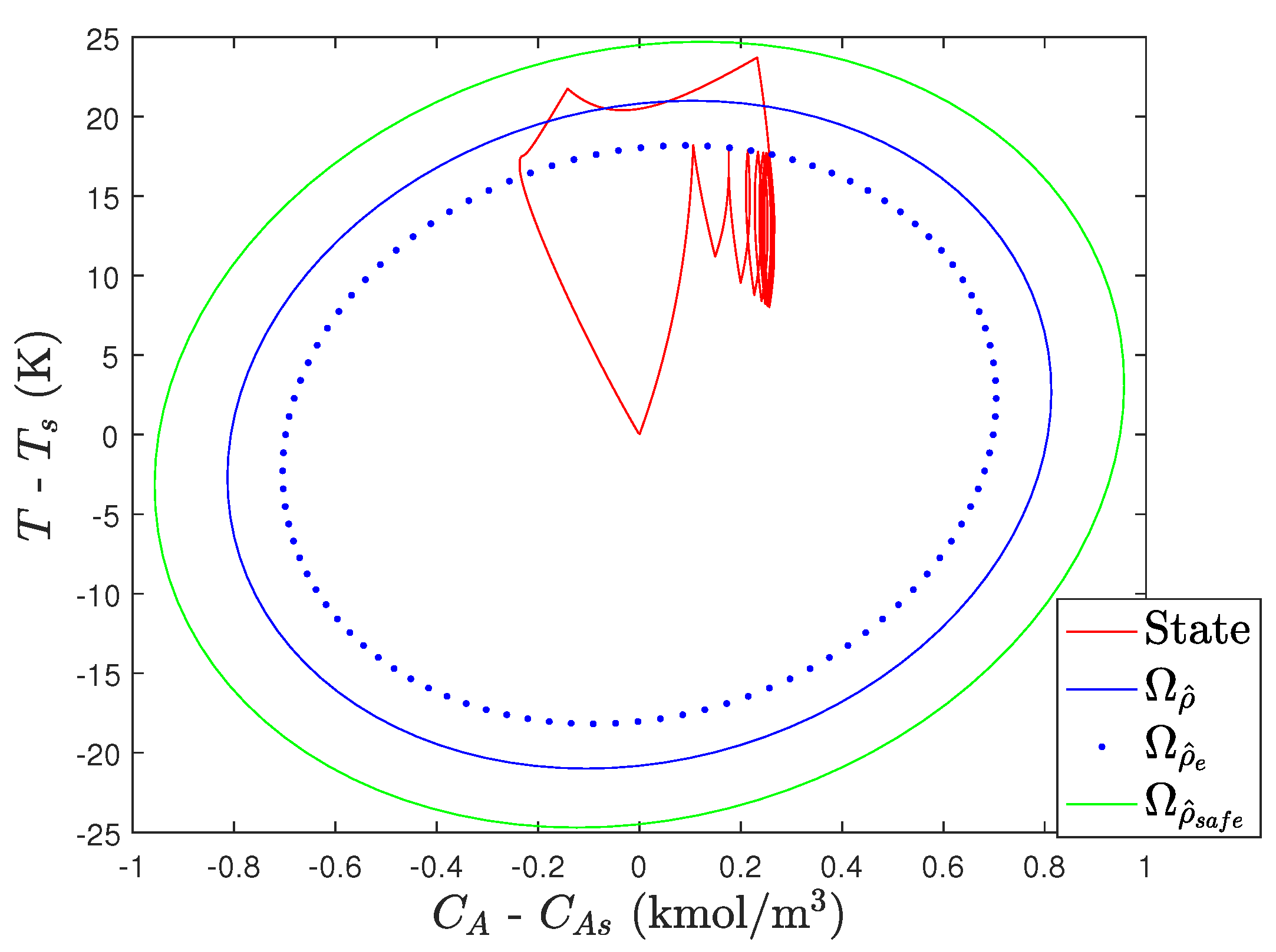
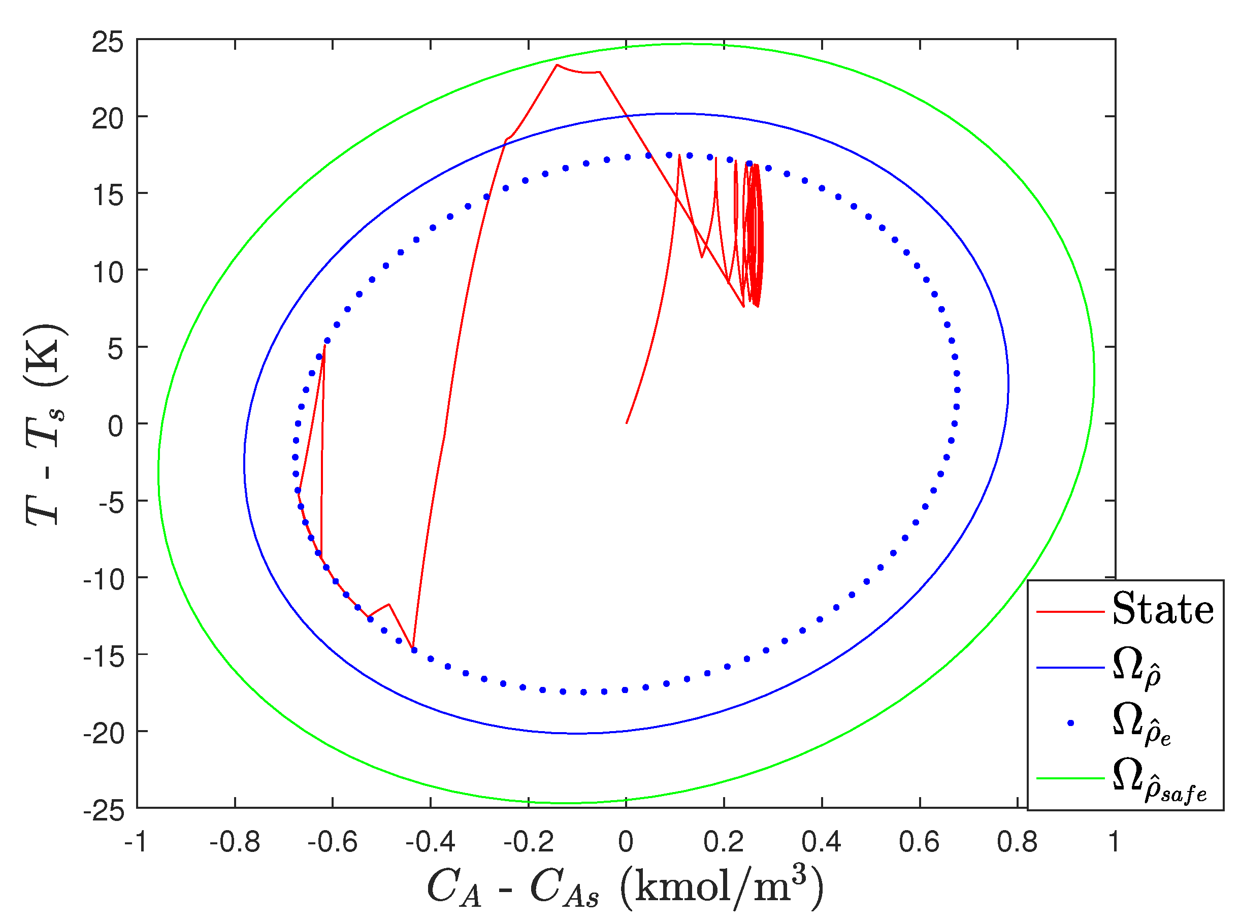
Second, at a chemical plant, anomalies may be considered to be either those which pose an immediate hazard to humans and the environment and are considered to require plant shutdown upon detection or those which do not. When the anomaly detected requires plant shutdown, generally the safety system is used to take extreme actions like cutting feeds to shut down the plant as quickly as possible; these generally have a prespecified nature (e.g., closing the feed valve). Anomalies that do not present immediate hazards to humans may either result in sufficiently small plant/model mismatch that the controller is robust against or the plant/model mismatch could cause subsequent control actions to drive the closed-loop state out of the expected region of process operation (at which point, the anomaly may be a hazard). We consider that characterizing conditions under which closed-loop stability is not lost in the second case may constitute steps in moving toward verification of EMPC for the process industries with adaptive model updates in the presence of changing process dynamics.

3.2.1. Automated Response to Anomalies: Formulation and Implementation Strategy

In the next section, we will present theoretical results regarding conditions under which an LEMPC could be conservatively designed to handle anomalies of different types in the sense that closed-loop stability would not be lost upon the occurrence of an anomaly or that impending loss of closed-loop stability could be detected by defining a region ${\mathsf{\Omega }}_{{\widehat{\rho }}_{samp,q}}$ (a superset of ${\mathsf{\Omega }}_{{\widehat{\rho }}_q}$) which the closed-loop state should not leave unless the anomaly has been significant and the model used by the LEMPC should be attempted to be reidentified to try to maintain closed-loop stability. If the closed-loop state leaves ${\mathsf{\Omega }}_{{\widehat{\rho }}_{samp,q}}$, however, it has also left ${\mathsf{\Omega }}_{{\widehat{\rho }}_q}$, so that the LEMPC of Equation (24) may not be feasible. For this reason, the implementation strategy below suggests that, if the closed-loop state leaves ${\mathsf{\Omega }}_{{\widehat{\rho }}_{samp,q}}$, $h_{NL,q}$ should be applied to the process so that a control law with no feasibility issues is used.

The implementation strategy proposed below relies on the existence of two controllers $h_{NL,q}$ and $h_{NL,q+1}$, where $h_{NL,q}$ can stabilize the origin of the nominal closed-loop system of Equation (10) and $h_{NL,q+1}$ can stabilize the origin of the nominal closed-loop system of Equation (10) with respect to the $q+1$th model. Specifically, before the change in the underlying process dynamics that occurs at $t_{s,i+1}$ is detected at $t_{d,q}$, the process is operated under the LEMPC with the qth empirical model. After the change is detected (in a worst case via the closed-loop state leaving ${\mathsf{\Omega }}_{{\widehat{\rho }}_q}$), a worst-case bound $t_{h,q}$ is placed on the time available until the model must be updated at time $t_{ID,q}$ to the $q+1$th empirical model to prevent the closed-loop state from leaving a characterizable operating region.

We consider the following implementation strategy for carrying out the above methodology:

• At $t_0$, the $i=1$ first-principles model (Equation (1)) describes the dynamics of the process. The $q=1$ empirical model (Equation (10)) is used to design the LEMPC of Equation (24). An index $i_{hx}$ is set to 0. An index $\zeta$ is set to 0. Go to step 2.
• At $t_{s,i+1}$, the underlying dynamic model of Equation (1) changes to the $i+1$th model. The LEMPC is not yet alerted that the anomaly has occurred; the model used in the LEMPC is not changed despite the change in the underlying process dynamics. Go to step 3.
• While $t_{s,i+1}<t_k<t_{s,i+2}$, apply a detection method to determine if an anomaly has occurred. If an anomaly is detected, set $\zeta =1$ and $t_{d,k}=t_k$. Else, $\zeta =0$. If $x(t_k)\notin {\mathsf{\Omega }}_{{\widehat{\rho }}_q}$ but $\zeta =0$, set $\zeta =1$ and $t_{d,k}=t_k$. Go to step 4.
• If $i_{hx}=1$, go to step 4a. Else, if $\zeta =1$, go to step 4b, or if $\zeta =0$, go to step 4c. If $t_k>t_{s,i+2}$, go to step 5.

  (a)

  If $x(t_k)\in {\mathsf{\Omega }}_{{\widehat{\rho }}_{q+1}}$, operate the process under the LEMPC of Equation (24) with $q\leftarrow q+1$ and set $i_{hx}=0$. Else, apply $h_{NL,q+1}(x(t_k))$ to the process. Return to step 3. $t_k\leftarrow t_{k+1}$.

  (b)

  If $(t_{k+1}-t_{d,q})<t_{h,q}$, gather online data to develop an improved process model as well as updated functions ${\widehat{V}}_{q+1}$ and $h_{NL,q+1}(x)$ and an updated stability region ${\mathsf{\Omega }}_{{\widehat{\rho }}_{q+1}}$ around the steady-state of the new empirical model but do not yet update the LEMPC and control the process using the prior LEMPC. Else, if $(t_{k+1}-t_{d,q})\ge t_{h,q}$, set $i_{hx}=1$ and apply $h_{NL,q+1}(x(t_k))$. Return to step 3. $t_k\leftarrow t_{k+1}$.

  (c)

  Operate the process under the LEMPC of Equation (24) that was used at the prior sampling time. Return to step 3. $t_k\leftarrow t_{k+1}$.

• If $t_k>t_{s,i+2}$, a process dynamics change occurred at $t_{s,i+2}$. Set $t_{s,i+1}\leftarrow t_{s,i+2}$ and $t_k\leftarrow t_{k+1}$. Return to step 2 with $\zeta =0$ and $i_{hx}=0$. Else, if $t_k<t_{s,i+2}$, $t_k\leftarrow t_{k+1}$; return to step 3.

We note that we do not specify the detection method to be used in step 3, but the use of a sufficiently conservative ${\mathsf{\Omega }}_{{\widehat{\rho }}_q}$ (in a sense to be clarified in the following section) allows a worst-case detection mechanism to be that the closed-loop state exits ${\mathsf{\Omega }}_{{\widehat{\rho }}_q}$ in step 3. We consider that each $t_{s,i+1}$ and $t_{s,i+2}$ are separated by a sufficient period of time such that no second change in the underlying process dynamics occurs before the first change has resulted in an update in the dynamic model and the closed-loop state is within ${\mathsf{\Omega }}_{{\widehat{\rho }}_{q+1}}$.

Remark 7.

A significant difference between the proposed procedure and that in References [53,54], which also involves switched systems under LEMPC, is that Reference [53] assumes that the time at which the model is to be switched is known a priori. In handling of anomalies, this cannot be known; therefore, the proposed approach corresponds to LEMPC for switched systems with unknown switching times. We place bounds in the next section on a number of properties of the LEMPC of Equation (24) for this case to demonstrate the manner in which closed-loop stability guarantees depend on, for example, how large the possible changes in the process model could be when they occur. The goal is to provide a perspective on the timeframes available for detecting various anomalies without loss of closed-loop stability, which could aid in verification and self-design studies for EMPC.

3.2.2. Automated Response to Anomalies: Stability and Feasibility Analysis

According to the implementation strategy above, when an anomaly occurs that changes the underlying process dynamics, one of two things will happen: (1) the model used in Equation (24b) remains the same or (2) the change in the underlying process dynamics is detected and the model used in Equation (24b) is changed within a required timeframe to a new model (i.e., q is incremented by one in Equation (10)). In this section, we present the conditions under which closed-loop stability can be maintained in either case. For readability, proofs of theorems presented in this section are available in the Appendix.

We first present several propositions. The first defines the maximum difference between the process model of Equation (1) and that of Equation (10) over time when the two models are initialized from the same state, as long as the states of both systems are kept within a level set of ${\widehat{V}}_q$ which is also contained within the stability region around the steady-state for the model of Equation (1) and as long as there is no change in the underlying dynamics. The second sets an upper bound on the difference between the value of ${\widehat{V}}_q$ at any two points in ${\mathsf{\Omega }}_{{\widehat{\rho }}_q}$. The third provides the closed-loop stability properties of the closed-loop system of Equation (10) under the controller $h_{NL,q}$.

Proposition 1

([51]). Consider the systems

$$\begin{array}{c}{\dot{\overline{x}}}_{a,i,q}={\overline{f}}_{i,q}({\overline{x}}_{a,i,q}(t),{\overline{u}}_q(t),w_i(t))\hfill \end{array}$$

(49a)

$$\begin{array}{c}{\dot{\overline{x}}}_{b,q}={\overline{f}}_{NL,q}({\overline{x}}_{b,q}(t),{\overline{u}}_q(t))\hfill \end{array}$$

(49b)

with initial states ${\overline{x}}_{a,i,q}(t_0)={\overline{x}}_{b,q}(t_0)=\overline{x}(t_0)$ contained within ${\mathsf{\Omega }}_{{\widehat{\rho }}_{q,i}}$, with $t_0=0$, ${\overline{u}}_q\in U_q$, and $w_i\in W_i$. If ${\overline{x}}_{a,i,q}(t)$ and ${\overline{x}}_{b,q}(t)$ remain within ${\mathsf{\Omega }}_{{\widehat{\rho }}_{q,i}}$ for $t\in [0,T]$, then there exists a function $f_{W,i,q}(·)$ such that:

$$\begin{array}{c}|{\overline{x}}_{a,i,q}(t)-{\overline{x}}_{b,q}(t)|\le f_{W,i,q}(t)\hfill \end{array}$$

(50)

with:

$$\begin{array}{c}{f}_{W,i,q}(t):=\frac{L_{w,i,q}{\theta }_i+M_{err,i,q}}{L_{x,i,q}}(e^{L_{x,i,q}t}-1)\hfill \end{array}$$

(51)

where $M_{err,i,q}>0$ is defined by:

$$\begin{array}{c}|{\overline{f}}_{i,q}(x,u,0)-{\overline{f}}_{NL,q}(x,u)|\le M_{err,i,q}\hfill \end{array}$$

(52)

for all x contained in ${\mathsf{\Omega }}_{{\widehat{\rho }}_{q,i}}$ and $u\in U_q$.

Proposition 2

([24,55]). Consider the Lyapunov function ${\widehat{V}}_q(·)$ of the nominal system of Equation (10) under the controller $h_{NL,q}(·)$ that meets Equation (12). There exists a quadratic function $f_{V,q}(·)$ such that:

$$\begin{array}{c}{\widehat{V}}_q(x)\le {\widehat{V}}_q(x^{\prime })+f_{V,q}(|x-x^{\prime }|)\hfill \end{array}$$

(53)

for all $x,{\overline{x}}^{\prime }\in {\mathsf{\Omega }}_{{\widehat{\rho }}_{safe,q}}$ with

$$\begin{array}{c}{f}_{V,q}(s):={\widehat{\alpha }}_{4,q}({\widehat{\alpha }}_{1,q}^{-1}({\widehat{\rho }}_q))s+M_{v,q}{s}^2\hfill \end{array}$$

(54)

where $M_{v,q}$ is a positive constant.

Proposition 3

([51]). Consider the closed-loop system of Equation (10) under $h_{NL,q}({\overline{x}}_{b,q})$ that satisfies the inequalities of Equation (12) in sample-and-hold. Let $\Delta >0$, ${\widehat{ϵ}}_{W,q}>0$, and ${\widehat{\rho }}_{safe,q}>{\widehat{\rho }}_q>{\widehat{\rho }}_{e,q}>{\widehat{\rho }}_{{min}_q}>{\widehat{\rho }}_{s,q}>0$ satisfy the following:

$$-{\widehat{\alpha }}_{3,q}({{\widehat{\alpha }}_{2,q}}^{-1}({\widehat{\rho }}_{s,q}))+L_{L,q}{M}_{L,q}\Delta \le -{\widehat{ϵ}}_{W,q}/\Delta$$

(55)

$${\widehat{\rho }}_{{min}_q}:=max\{{\widehat{V}}_q({\overline{x}}_{b,q}(t+\Delta ))\hspace{1em}:\hspace{1em}{\widehat{V}}_q({\overline{x}}_{b,q}(t))\le {\widehat{\rho }}_{s,q}\}.$$

(56)

If ${\overline{x}}_{b,q}(0)\in {\mathsf{\Omega }}_{{\widehat{\rho }}_{safe,q}}$, then,

$${\widehat{V}}_q({\overline{x}}_{b,q}(t_{k+1}))-{\widehat{V}}_q({\overline{x}}_{b,q}(t_k))\le -{\widehat{ϵ}}_{W,q}$$

(57)

for ${\overline{x}}_{b,q}(t_k)\in {\mathsf{\Omega }}_{{\widehat{\rho }}_{safe,q}}/{\mathsf{\Omega }}_{{\widehat{\rho }}_{s,q}}$ and the state trajectory ${\overline{x}}_{b,q}(t)$ of the closed-loop system is always bounded in ${\mathsf{\Omega }}_{{\widehat{\rho }}_{safe,q}}$ for $t\ge 0$ and is ultimately bounded in ${\mathsf{\Omega }}_{{\widehat{\rho }}_{{min}_q}}$.

The next proposition bounds the error between the actual process state and a prediction of the process state using an empirical model initialized from the same value of the process state over a period of time in which the underlying process dynamics change, but the empirical model is not updated. This requires overlap in stability regions for the ith and $i+1$th models of Equation (1) and for the qth model of Equation (10) within ${\mathsf{\Omega }}_{{\widehat{\rho }}_{q,i}}$ while the qth model is used. The proof of this proposition is available in Appendix A.

Proposition 4.

Consider the following systems:

$${\dot{\overline{x}}}_{a,i,q}={\overline{f}}_{i,q}({\overline{x}}_{a,i,q}(t),{\overline{u}}_q(t),w_i(t))$$

(58)

$${\dot{\overline{x}}}_{b,q}={\overline{f}}_{NL,q}({\overline{x}}_{b,q}(t),{\overline{u}}_q(t))$$

(59)

$${\dot{\overline{x}}}_{a,i+1,q}={\overline{f}}_{i+1,q}({\overline{x}}_{a,i+1,q}(t),{\overline{u}}_q(t),w_{i+1}(t))$$

(60)

with initial states ${\overline{x}}_{a,i,q}(t_0)={\overline{x}}_{b,q}(t_0)\in {\mathsf{\Omega }}_{{\widehat{\rho }}_{q,i}}$ with $t_0=0$, ${\overline{u}}_q\in U_q$, $w_i\in W_i$, and $w_{i+1}\in W_{i+1}$. Also, ${\overline{x}}_{a,i,q}(t_{s,i+1})={\overline{x}}_{a,i+1,q}(t_{s,i+1})$. If ${\overline{x}}_{a,i,q}(t)$, ${\overline{x}}_{b,q}(t)$, ${\overline{x}}_{a,i+1,q}(t)\in {\mathsf{\Omega }}_{{\widehat{\rho }}_{q,i}}$ for $t\in [0,t_1]$ and

$$|{\overline{f}}_{i+1,q}({\overline{x}}_{a,i+1,q}(s),{\overline{u}}_q(s),w_{i+1}(s))-{\overline{f}}_{i,q}({\overline{x}}_{a,i,q}(s),{\overline{u}}_q(s),w_i(s))|\le M_{change,i,q}$$

(61)

for all ${\overline{x}}_{a,i,q},{\overline{x}}_{a,i+1,q}\in {\mathsf{\Omega }}_{{\widehat{\rho }}_{q,i}}$, ${\overline{u}}_q\in U_q$, $w_i\in W_i$, and $w_{i+1}\in W_{i+1}$, then

$$|{\overline{x}}_{a,i,q}(t)-{\overline{x}}_{b,q}(t)|\le f_{W,i,q}(t)$$

(62)

where $f_{W,i,q}(t)$ is defined in Equation (51) for $t\in [0,t_{s,i+1}]$ and

$$\begin{array}{c}|{\overline{x}}_{a,i+1,q}(t)-{\overline{x}}_{b,q}(t)|\le f_{W,i,q}(t_{s,i+1}-t_0)+(M_{change,i,q})(t-t_{s,i+1})+\frac{L_{w,i,q}{\theta }_i+M_{err,i,q}}{L_{x,i,q}}(e^{L_{x,i,q}t}-e^{L_{x,i,q}{t}_{s,i+1}})\end{array}$$

(63)

for $t\in [t_{s,i+1},t_1]$.

The following theorem provides the conditions under which, when no change in the underlying dynamic model occurs throughout the time of operation and $x(t_k)\in {\mathsf{\Omega }}_{{\widehat{\rho }}_q}$, the LEMPC of Equation (24) designed based on $h_{NL,q}$ and the qth empirical model of Equation (10) guarantees that the closed-loop state is maintained within ${\mathsf{\Omega }}_{{\widehat{\rho }}_q}$ over time and is ultimately bounded in a neighborhood of the origin of the model of Equation (10).

Theorem 1

([51]). Consider the closed-loop system of Equation (1) under the LEMPC of Equation (24) based on the controller $h_{NL,q}(x)$ that satisfies the inequalities in Equation (12). Let ${ϵ}_{W,i,q}>0$, $\Delta >0$, $N\ge 1$, and ${\widehat{\rho }}_q>{\widehat{\rho }}_{e,q}>{\widehat{\rho }}_{min,i,q}>{\widehat{\rho }}_{s,q}>0$ satisfy the following:

$$\begin{array}{c}-{\widehat{\alpha }}_{3,q}({\widehat{\alpha }}_{2,q}^{-1}({\widehat{\rho }}_{e,q}))+{\widehat{\alpha }}_{4,q}({\widehat{\alpha }}_{1,q}^{-1}({\widehat{\rho }}_q))M_{err,i,q}+L_{x,i,q}^{\prime }{M}_i\Delta +L_{w,i,q}^{\prime }{\theta }_i\le -{ϵ}_{W,i,q}/\Delta \hfill \end{array}$$

(64)

$$\begin{array}{c}{\widehat{\rho }}_{e,q}\le {\widehat{\rho }}_q-f_{V,q}(f_{W,i,q}(\Delta ))\hfill \end{array}$$

(65)

If $x(0)\in {\mathsf{\Omega }}_{{\widehat{\rho }}_q}$ and Proposition 3 is satisfied, then the state trajectory ${\overline{x}}_{a,i,q}(t)$ of the closed-loop system is always bounded in ${\mathsf{\Omega }}_{{\widehat{\rho }}_q}$ for $t\ge 0$. Furthermore, if $t>t^{\prime }$ and

$$\begin{array}{c}-{\widehat{\alpha }}_{3,q}({\widehat{\alpha }}_{2,q}^{-1}({\widehat{\rho }}_{s,q}))+{\widehat{\alpha }}_{4,q}({\widehat{\alpha }}_{1,q}^{-1}({\widehat{\rho }}_q))M_{err,i,q}+L_{x,i,q}^{\prime }{M}_i\Delta +L_{w,i,q}^{\prime }{\theta }_i\le -{ϵ}_{W,i,q}/\Delta \hfill \end{array}$$

(66)

then the state trajectory $x_{a,i}(t)$ of the closed-loop system is ultimately bounded in ${\mathsf{\Omega }}_{{\widehat{\rho }}_{min,i,q}}$ and defined as follows:

$${\widehat{\rho }}_{min,i,q}:=max\{{\widehat{V}}_q({\overline{x}}_{a,i,q}(t+\Delta )) | {\widehat{V}}_q({\overline{x}}_{a,i,q}(t))\le {\widehat{\rho }}_{s,q}\}$$

(67)

The prior theorem provided conditions under which the closed-loop state is maintained within ${\mathsf{\Omega }}_{{\widehat{\rho }}_q}$ in the absence of changes in the dynamic model. In the following theorem, we provide sufficient conditions under which the closed-loop state is maintained in ${\mathsf{\Omega }}_{{\widehat{\rho }}_q}$ after $t_{s,i}$. The proof of this result is presented in Appendix B.

Theorem 2.

Consider the closed-loop system of Equation (1) under the LEMPC of Equation (24) with $h_{NL,q}$ meeting Equation (12), where the conditions of Propositions 3 and 4 hold and where ${\mathsf{\Omega }}_{{\widehat{\rho }}_{safe,q}}$ is contained in both ${\mathsf{\Omega }}_{{\rho }_i}$ and ${\mathsf{\Omega }}_{{\rho }_{i+1}}$. If $t_{s,i+1}\in [t_k,t_{k+1})$, such that, after $t_{s,i+1}$, the system of Equation (1) is controlled by the LEMPC of Equation (24), where $x_{a,i}(t_{s,i+1})=x_{a,i+1}(t_{s,i+1})\in {\mathsf{\Omega }}_{{\widehat{\rho }}_q}$, and if the following hold true,

$$\begin{array}{c}-{\widehat{\alpha }}_{3,q}({\widehat{\alpha }}_{2,q}^{-1}({\widehat{\rho }}_{e,q}))+{\widehat{\alpha }}_{4,q}({\widehat{\alpha }}_{1,q}^{-1}({\widehat{\rho }}_q))M_{err,p,q}+L_{x,p,q}^{\prime }{M}_p\Delta +L_{w,p,q}^{\prime }{\theta }_p\le -{ϵ}_{W,p,q}/\Delta \hfill \end{array}$$

(68)

$$\begin{array}{c}{\widehat{\rho }}_{e,q}\le {\widehat{\rho }}_q-f_{V,q}(f_{W,p,q}(\Delta ))\hfill \end{array}$$

(69)

for both $p=i$ and $p=i+1$, and

$$\begin{array}{c}{\widehat{\rho }}_{e,q}+f_{V,q}(f_{W,i,q}\Delta +(M_{change,i})\Delta +\frac{L_{w,i,q}{\theta }_i+M_{err,i,q}}{L_{x,i,q}}(e^{L_{x,i,q}\Delta }-e^{L_{x,i,q}{t}_{s,i+1}}))\le {\widehat{\rho }}_q\hfill \end{array}$$

(70)

$$\begin{array}{c}-{\widehat{\alpha }}_{3,q}({\widehat{\alpha }}_{2,q}^{-1}({\widehat{\rho }}_{e,q}))+{\widehat{\alpha }}_{4,q}({\widehat{\alpha }}_{1,q}^{-1}({\widehat{\rho }}_q))M_{err,i,q}+L_{x,i,q}^{\prime }{M}_i\Delta +L_{w,i,q}^{\prime }{\theta }_i+{\widehat{\alpha }}_{4,q}({\widehat{\alpha }}_{1,q}^{-1}({\widehat{\rho }}_q))M_{change,i,q}+L_{x,i+1,q}^{\prime }{M}_{i+1}\Delta \hfill \\ \hspace{1em}\hspace{1em}+L_{w,i+1,q}^{\prime }{\theta }_{i+1}\le -{ϵ}_{W,i,q}^{\prime }/\Delta \hfill \end{array}$$

(71)

then the closed-loop state is bounded in ${\mathsf{\Omega }}_{{\widehat{\rho }}_q}$ for all $t\ge 0$.

We highlight that these conditions are conservative and not intended to form the least conservative bounds possible. However, they do help to elucidate some of the factors which impact whether a model used in an LEMPC will need to be reidentified to continue to maintain closed-loop stability when the underlying dynamics change, such as the extent to which the dynamics change. The above theorem indicates that, if ${\mathsf{\Omega }}_{{\widehat{\rho }}_q}$ is initially chosen in a sufficiently conservative fashion and the empirical model is sufficiently close to the underlying process dynamics before the model change, closed-loop stability may be maintained even after the underlying dynamics change if the model changes are such that the empirical model remains sufficiently close to the new dynamic model after the change. In general, anomalies may occur that could violate the conditions of Theorem 2. The result of this could be that the closed-loop state may leave ${\mathsf{\Omega }}_{{\widehat{\rho }}_q}$. In this case, it is helpful to characterize conditions under which changes in the underlying dynamics that could be destabilizing could be detected, triggering a model update and controller redesign for the new dynamic model to stabilize the closed-loop system. Therefore, the following theorem characterizes the length of time that the closed-loop state can remain in ${\mathsf{\Omega }}_{{\widehat{\rho }}_{safe,q}}$ after a change in the underlying process dynamics occurs if the conditions of Theorem 2 are not met. This can be used in determining how quickly a model reidentification algorithm would need to successfully provide a new model for the LEMPC of Equation (24) for closed-loop stability to be maintained as a function of factors such as the extent that the new model deviates from the empirical model used in the LEMPC when the underlying dynamics change, the sampling period, and the conservatism in the selection of ${\widehat{\rho }}_q$. The proof of this theorem is presented in Appendix C.

Theorem 3.

Consider the closed-loop system of Equation (1) under the LEMPC of Equation (24) with $h_{NL,q}$ meeting Equation (12) and Proposition 3, where ${\mathsf{\Omega }}_{{\widehat{\rho }}_{safe,q}}$ is contained in both ${\mathsf{\Omega }}_{{\rho }_i}$ and ${\mathsf{\Omega }}_{{\rho }_{i+1}}$. If at $t=t_{s,i+1}$, where $t_{s,i+1}\in [t_k,t_{k+1})$, such that, after $t_{s,i+1}$, the system of Equation (1) is controlled by the LEMPC of Equation (24), where $x_{a,i}(t_{s,i+1})=x_{a,i+1}(t_{s,i+1})\in {\mathsf{\Omega }}_{{\widehat{\rho }}_{safe,q}}$, then if the following hold true with ${\widehat{\rho }}_{safe,q}>{\widehat{\rho }}_{samp,q}>{\widehat{\rho }}_q>{\widehat{\rho }}_{q,e}$, ${\widehat{\rho }}_{q,e}>{\widehat{\rho }}_{min,q,i}>{\widehat{\rho }}_{s,q}>0$, and ${\widehat{\rho }}_{q,e}>{\widehat{\rho }}_{min,i+1,q}>{\widehat{\rho }}_{s,q}>0$:

$$\begin{array}{c}-{\widehat{\alpha }}_{3,q}({\widehat{\alpha }}_{2,q}^{-1}({\widehat{\rho }}_{s,q}))+{\widehat{\alpha }}_{4,q}({\widehat{\alpha }}_{1,q}^{-1}({\widehat{\rho }}_q))M_{err,i+1,q}+L_{x,i+1,q}^{\prime }{M}_{i+1}\Delta +L_{w,i+1,q}^{\prime }{\theta }_{i+1}\le {ϵ}_{W,i+1,q}/\Delta \hfill \end{array}$$

(72)

$$\begin{array}{c}{\widehat{\rho }}_{e,q}+f_{V,q}(f_{W,i,q}\Delta +(M_{change,i,q})\Delta +\frac{L_{w,i,q}{\theta }_i+M_{err,i,q}}{L_{x,i,q}}(e^{L_{x,i,q}\Delta }-e^{L_{x,i,q}{t}_{s,i+1}}))\le {\widehat{\rho }}_{samp,q}\hfill \end{array}$$

(73)

$$\begin{array}{c}{\widehat{\rho }}_q+f_{V,q}(f_{W,i,q}\Delta +(M_{change,i,q})\Delta +\frac{L_{w,i,q}{\theta }_i+M_{err,i,q}}{L_{x,i,q}}(e^{L_{x,i,q}\Delta }-e^{L_{x,i,q}{t}_{s,i+1}}))\le {\widehat{\rho }}_{samp,q}\hfill \end{array}$$

(74)

$${\widehat{\rho }}_{e,q}+f_{V,q}(f_{W,i+1,q}(\Delta ))\le {\widehat{\rho }}_{samp,q}$$

(75)

$${\widehat{\rho }}_q+{ϵ}_{W,i+1,q}\le {\widehat{\rho }}_{samp,q}$$

(76)

as well as Equations (65)–(67), then if $x(t_{s,i+1})\in {\mathsf{\Omega }}_{{\widehat{\rho }}_q}$ and ${\mathsf{\Omega }}_{{\widehat{\rho }}_{min,i+1,q}}\subset {\mathsf{\Omega }}_{{\widehat{\rho }}_{samp,q}}$ and the change to the model is not detected until a sampling time $t_{d,q}$ with $\overline{x}(t_{d,q})\in {\mathsf{\Omega }}_{{\widehat{\rho }}_{safe,q}}/{\mathsf{\Omega }}_{{\widehat{\rho }}_q}$ ($\overline{x}(t_{d,q})\in {\mathsf{\Omega }}_{{\widehat{\rho }}_{samp,q}}\subset {\mathsf{\Omega }}_{{\widehat{\rho }}_{safe,q}}$) after which $h_{NL,q}$ is used to control the system in sample-and-hold, then the number of sampling periods between $t_{ID,q}$ and $t_{d,q}$ within which the model in the LEMPC can be updated to a new model meeting Equation (65) with i replaced by $i+1$ and q replaced by $q+1$ without the closed-loop state exiting ${\mathsf{\Omega }}_{{\widehat{\rho }}_{safe,q}}$ is given by $t_{h,q}=\mathit{floor}(\frac{({\widehat{\rho }}_{safe,q}-{\widehat{\rho }}_{samp,q})}{{ϵ}_{W,i,q}^{\prime }})$, where floor represents the “floor” function that returns the largest integer less than the value of the argument. $\overline{x}(t)$ refers either to ${\overline{x}}_{a,i+1,q}(t)$ or ${\overline{x}}_{a,i,q}(t)$, depending on whether $t_{s,i+1}$ is within the sampling period preceding the closed-loop state exiting ${\mathsf{\Omega }}_{{\widehat{\rho }}_q}$.

The following theorem provides the conditions under which the closed-loop state is maintained within ${\mathsf{\Omega }}_{{\widehat{\rho }}_{safe,q+1}}$ for all times after $t_{ID,q}$ and is driven into ${\mathsf{\Omega }}_{{\widehat{\rho }}_{q+1}}$ after the model reidentification. The proof of the result is presented in Appendix D.

Theorem 4.

If ${\mathsf{\Omega }}_{{\widehat{\rho }}_{safe,q}}\subset {\mathsf{\Omega }}_{{\widehat{\rho }}_{safe,q+1}}$ and if both ${\mathsf{\Omega }}_{{\widehat{\rho }}_{safe,q}}$ and ${\mathsf{\Omega }}_{{\widehat{\rho }}_{safe,q+1}}$ are contained in ${\mathsf{\Omega }}_{{\rho }_i}$ and ${\mathsf{\Omega }}_{{\rho }_{i+1}}$, then if $h_{NL,q+1}$ is used to control the system after $t_{ID,q}$ while $x(t_k)\in {\mathsf{\Omega }}_{{\widehat{\rho }}_{safe,q+1}}/{\mathsf{\Omega }}_{{\widehat{\rho }}_{q+1}}$ with the conditions of Equations (65) and (66) met for the $q+1$th empirical model for the $i+1$th dynamic system and the LEMPC of Equation (24) using the $q+1$th empirical model of Equation (10) is used to control the system for all times after $x(t_k)\in {\mathsf{\Omega }}_{{\widehat{\rho }}_{q+1}}$, then the closed-loop state is then maintained within ${\mathsf{\Omega }}_{{\widehat{\rho }}_{safe,q+1}}$ until it enters ${\mathsf{\Omega }}_{{\widehat{\rho }}_{q+1}}$ and is then maintained in ${\mathsf{\Omega }}_{{\widehat{\rho }}_{q+1}}$ for all subsequent sampling times.

Remark 8.

From a verification standpoint, the proofs above move toward addressing the question of what may happen if a controller is designed and even tested for certain conditions, but the process dynamics change. It provides a theoretical characterization of conditions under which action would subsequently need to be taken as well as indications of the time available to take the subsequent action. However, the results above may be difficult to utilize directly in developing an online monitoring scheme, as many of the theoretical conditions rely on knowing properties of the current and updated models that would likely not be characterizable or would not be known until after the anomaly occurred. However, these still may aid in gaining an understanding of different possibilities. For example, a conservative stability region ${\mathsf{\Omega }}_{{\widehat{\rho }}_q}$ suggests that larger anomalies could still be detected and mitigated by a combined detection and reidentification procedure without loss of closed-loop stability. Earlier detection may provide more time for reidentification.

Remark 9.

If there is an indication from detection methods that are not based on the closed-loop state leaving the stability region that the underlying dynamics may have changed but that the closed-loop state has not yet left ${\mathsf{\Omega }}_{{\widehat{\rho }}_q}$, then until the closed-loop state leaves ${\mathsf{\Omega }}_{{\widehat{\rho }}_q}$, online experiments (e.g., modifying the objective function as in Reference [51]) could be performed if they do not impact the constraint set to attempt to probe whether the dynamics are more consistent with the prior process model or the potential model postulated after the anomaly is suggested. This may be a method for attempting to detect the changes before the closed-loop state leaves ${\mathsf{\Omega }}_{{\widehat{\rho }}_q}$, which could allow larger changes in the process model to be handled practically than could be guaranteed to be handled in the theorems above, as the magnitude of the deviations in the dynamic model allowed above without loss of closed-loop stability depends on the distance between ${\mathsf{\Omega }}_{{\widehat{\rho }}_{safe,q}}$ and ${\mathsf{\Omega }}_{{\widehat{\rho }}_{samp,q}}$. However, it is also highlighted that the above is a conservative result, meaning that, in general, larger changes may be able to be handled without loss of closed-loop stability.

Remark 10.

The above results can be used to comment on why giving greater flexibility to the process after an anomaly to handle it could introduce additional complexity. Specifically, consider the possibility that some actuators may not typically be used for control but could be considered for use after an anomaly (similar to how safety systems activate for chemical processes, but in this case, they would not act according to a prespecified logic but might be able to be manipulated in either an on-off or continuous manner to give the process additional capabilities for handling the anomaly). It is noted that this would constitute dynamics not previously considered. According to the proofs above, one way to guarantee closed-loop stability in the presence of sufficiently small disturbances is to cause the dynamics after they change to not differ too radically from those assumed before the change and used in the prior dynamic model in the EMPC. If additional flexibility is given to the system, this would be an additional model that would have to match up well.

Remark 11.

The results above suggest that, if a model identification algorithm could be guaranteed to provide an accurate model with a small amount of data that could be gathered between when the closed-loop state leaves ${\mathsf{\Omega }}_{{\widehat{\rho }}_q}$ but before it leaves ${\mathsf{\Omega }}_{{\widehat{\rho }}_{safe,q}}$ (where the amount of data available in that timeframe could be known a priori by the number of measurements available in a given sampling period), then the model could be reidentified and placed within the LEMPC in a manner that is stabilizing.

Remark 12.

Instead of changes to the underlying dynamic model, anomalies may present changes in the constraint set (e.g., anomalies may change equipment material limitations (e.g., maximum shear stresses, which can change with temperature) used to place constraints on the state in an LEMPC). Because the above results assume that the stability region is fully contained within the state constraint set, the detection and response procedure above would need to ensure that there is no time at which the stability region is no longer fully included within the state constraint set under the new dynamic model. This may be handled by making ${\mathsf{\Omega }}_{{\widehat{\rho }}_{safe,q}}$ sufficiently conservative such that the closed-loop state never exits a region where the state constraints can be met under different dynamic models.

3.2.3. Automated Response to Unexpected Hazards: Application to a Chemical Process Example

In this section, we demonstrate concepts described above through a process example. This example considers a nonisothermal reactor in which an $A\to B$ reaction takes place, but the reactant inlet concentration $C_{A0}$ and the heat rate Q supplied by a jacket are adjusted by an LEMPC. The process model is as follows:

$${\dot{C}}_A=\frac{F}{V}(C_{A0}-C_A)-k_0{e}^{-\frac{E}{R_{g}T}}{C}_A^2$$

(77)

$$\dot{T}=\frac{F}{V}(T_0-T)-\frac{\Delta H{k}_0}{{\rho }_L{C}_p}{e}^{-\frac{E}{R_{g}T}}{C}_A^2+\frac{Q}{{\rho }_L{C}_{p}V}$$

(78)

where the parameters are listed in

Table 3. Parameters for the CSTR model of Equations (77) and (78).

Parameter	Value	Unit
V	1	m${}^3$
$T_0$	300	K
$k_0$	$8.46\times {10}^6$	m${}^3$/h·kmol
$C_p$	$0.231$	kJ/kg·K
${\rho }_L$	1000	kg/m${}^3$
F	5	m${}^3$/h
$R_g$	$8.314$	kJ/kmol·K
E	$5\times {10}^4$	kJ/kmol
$\Delta H$	$-1.15\times {10}^4$	kJ/kmol

and include the reactor volume V, inlet reactant temperature $T_0$, pre-exponential constant $k_0$, solution heat capacity $C_p$, solution density ${\rho }_L$, feed/outlet volumetric flow rate F, gas constant $R_g$, activation energy E, and heat of reaction $\Delta H$. The state variables are the reactant concentration $C_A$ and temperature T in the reactor, which can be written in deviation form from the operating steady-state vector $C_{As}=1.22$ kmol/m${}^3$, $T_s=438.2$ K, $C_{A0s}=4$ kmol/m${}^3$, and $Q_s=0$ kJ/h as $x={[x_1 x_2]}^T={[C_A-C_{As} T-T_s]}^T$ and $u={[u_1 u_2]}^T={[C_{A0}-C_{A0s} Q-Q_s]}^T$. The model of Equations (77) and (78) has the following form:

$$\dot{x}=\tilde{f}(x)+g(x)u$$

(79)

where $\tilde{f}$ represents a vector function derived from Equations (77) and (78) that is not multiplied by u and where $g(x)={[g_1 g_2]}^T={[\frac{F}{V} 0; 0 \frac{1}{{\rho }_L{C}_{p}V}]}^T$ represents the vector function which multiplies u in these equations.

The EMPC utilized to adjust the manipulated inputs $C_{A0}$ and Q utilizes the following stage cost (to maximize the production rate of the desired product) and physical bounds on the inputs:

$$L_e=-k_0{e}^{-E/(R_{g}T(\tau ))}{C}_A{(\tau )}^2$$

(80)

$$0.5\le C_{A0}\le 7.5 \mathrm{kmol}/\mathrm{m}{}^3$$

(81)

$$-5\times {10}^5\le Q\le 5\times {10}^5 \mathrm{kJ}/\mathrm{h}$$

(82)

Lyapunov-based stability constraints are also enforced (where a constraint of the form of Equation (22) is enforced at the end of every sampling time if $x(t_k)\in {\mathsf{\Omega }}_{{\widehat{\rho }}_e}$, and the constraint of the form of Equation (23) is enforced at $t_k$ when $x(t_k)\in {\mathsf{\Omega }}_{\widehat{\rho }}/{\mathsf{\Omega }}_{{\widehat{\rho }}_e}$ but then followed by a constraint of the form of Equation (22) at the end of all sampling periods after the first).

We will consider several simulations to demonstrate the developments above. In the first, we explore several aspects of the case in which there is a change in the underlying dynamics while the process is operated under LEMPC that is minor such that the closed-loop state does not leave ${\mathsf{\Omega }}_{\widehat{\rho }}$ after the change in the underlying dynamics. For this case, the Lyapunov function selected was ${\widehat{V}}_q=x^{T}Px$, with P given as follows:

$$P=\left[\begin{array}{cc}1200& 5\\ 5& 0.1\end{array}\right]$$

(83)

The Lyapunov-based controller $h_{NL,1}(x)$ was designed such that its first component $h_{NL,1,1}(x)=0$ kmol/m${}^3$ and its second component $h_{NL,1,2}(x)$ is computed as follows (Sontag’s formula [56]):

$$\begin{array}{c}\hfill h_{NL,1,2}(x)=\left\{\begin{array}{cc}-\frac{L_{\tilde{f}}{\widehat{V}}_q+\sqrt{L_{\tilde{f}}{\widehat{V}}_q^2+L_{{\tilde{g}}_2}{\widehat{V}}_q^4}}{L_{{\tilde{g}}_2}{\widehat{V}}_q},\hfill & \mathrm{if} L_{{\tilde{g}}_2}{\widehat{V}}_q\ne 0\hfill \\ 0,\hfill & \mathrm{if} L_{{\tilde{g}}_2}{\widehat{V}}_q=0\hfill \end{array}\right.\end{array}$$

(84)

Then, it is saturated at the input bounds of Equation (82) if they are met. $L_{\tilde{f}}{\widehat{V}}_q$ and $L_{{\tilde{g}}_2}{\widehat{V}}_q$ are Lie derivatives of ${\widehat{V}}_q$ with respect to the vector functions $\tilde{f}$ and ${\tilde{g}}_2$, respectively. $\widehat{\rho }$ and ${\widehat{\rho }}_e$ were taken from Reference [57] to be 300 and 225, respectively. The process state was initialized at $x_{init}={[-0.4 {\mathrm{kmol}/\mathrm{m}}^3 8 \mathrm{K}]}^T$, with controller parameters $N=10$ and $\Delta =0.01$ h. The process model of Equations (77) and (78) was integrated with the explicit Euler numerical integration method using an integration step size of ${10}^{-4}$ h within the LEMPC and of ${10}^{-5}$ h to simulate the process.

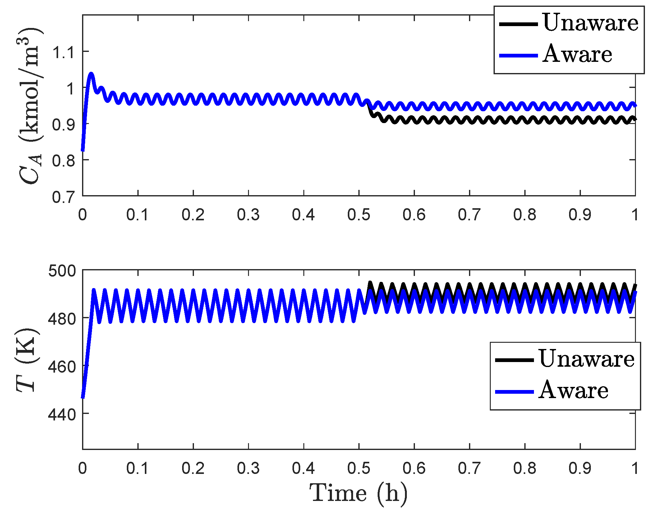
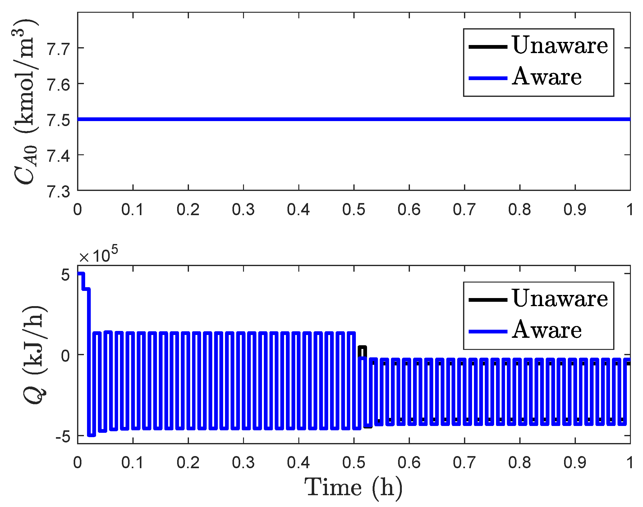
For this first simulation, we assume that a change in the underlying process dynamics occurs at 0.5 h that does not compromise closed-loop stability. Specifically, at 0.5 h, it is assumed that an additional source of heat arises outside the reactor such that the right-hand side of Equation (78) is modified by the addition of another term $Q_{extra}=300$ K/h. Figure 6 and Figure 7 show the process responses when the LEMPC is not aware of the change in the process dynamic model when it occurs and when it is aware of the change in the process dynamic model after it occurs such that it is fully compensated (i.e., an accurate process model is used in the LEMPC at all times, even after the dynamics change). In both cases, the closed-loop state was maintained within the stability region at all times. These simulations were carried out in MATLAB R2016b using fmincon with the default settings except for the increased iterations/function evaluations allowed, scaling $u_2$ down by ${10}^5$ and providing the steady-state input values as the initial guess for the optimization problem solution at each sampling time. No attempt was made to check whether the LEMPCs in the simulations located globally optimal solutions to the LEMPC optimization problems. However, the profit was higher than that at the steady-state around which the LEMPC was designed.

The oscillatory behavior of the states before 0.5 h is caused by the fact that the profit is maximized for this process at the boundary of ${\mathsf{\Omega }}_{{\widehat{\rho }}_e}$. Without plant-model mismatch, the LEMPC is able to maintain the closed-loop state exactly on the boundary of ${\mathsf{\Omega }}_{{\widehat{\rho }}_e}$ and therefore always operates the process using the constraint of Equation (22); however, when the plant-model mismatch occurs (induced by the use of different integration steps to simulate the process dynamic model within the LEMPC and for the simulation of the process under the computed control actions), the closed-loop state then exits ${\mathsf{\Omega }}_{{\widehat{\rho }}_e}$ when the LEMPC predicts it will stay inside of it under the control actions computed by the controller. The result is that the constraint of Equation (23) is then activated until the closed-loop state reenters ${\mathsf{\Omega }}_{{\widehat{\rho }}_e}$. This process of entering ${\mathsf{\Omega }}_{{\widehat{\rho }}_e}$, attempting to operate at its boundary, and then being kicked out only to be driven back in is the cause of the oscillatory response of the states and inputs in Figure 6 and Figure 7. It is noted, however, that though this behavior may be undesirable from, for example, an actuator wear perspective, it does not reflect a loss of closed-loop stability or a malfunction of the controller. The controller is in fact maintaining the closed-loop state within ${\mathsf{\Omega }}_{\widehat{\rho }}$ as it was designed to do; the fact that it does so in perhaps a visually unfamiliar fashion means that we have not specified in the control law that it should not do that, so it is not aware that an end user would find that behavior strange (if the oscillatory behavior is deemed undesirable, one could consider, for example, input rate of change constraints and potentially the benefits of the human response-based input rate of change strategy in the prior section for handling unexpected events).

In the case that the LEMPC is not aware of the change in the process dynamics, the profit is 32.7103, whereas when the LEMPC is aware of the change in the dynamics, the profit is 32.5833. Though these values are very close, an interesting note is that the profit when the LEMPC is not aware of the change in the underlying dynamics is slightly higher than when it is aware. Intuitively, one would expect an LEMPC with a more accurate process model to be able to locate a more economically optimal trajectory for the closed-loop state to follow than an LEMPC that cannot provide as accurate predictions. Part of the reason for the enhanced optimality in the case without knowledge of the change in the underlying dynamics, however, comes from the two-mode nature of LEMPC. In the case that the LEMPC is aware of the change in the underlying dynamics, it drives the closed-loop state to an operating condition that remains closer to the boundary of ${\mathsf{\Omega }}_{{\widehat{\rho }}_e}$ after 0.5 h than when it is not aware of the change in the underlying dynamics due to the plant/model mismatch being different in the different cases. The result is that the process accesses regions of state-space that lead to higher profits when the LEMPC does not know about the change in the dynamics than if the LEMPC knows more about the process dynamics.

The remainder of this example focuses on elucidating the conservativeness of the proposed approach. Specifically, we now consider the Lyapunov function selected as ${\widehat{V}}_q=x^{T}Px$, with P given as follows:

$$P=\left[\begin{array}{cc}2000& -10\\ -10& 3\end{array}\right]$$

(85)

Again, $h_{NL,1}(x)$ is designed such that $h_{NL,1,1}(x)=0$ kmol/m${}^3$, and $h_{NL,1,2}(x)$ is computed via Sontag’s formula but saturated at the input bounds of Equation (82) if they are met. $\widehat{\rho }$ and ${\widehat{\rho }}_e$ were taken to be 1300 and 975, respectively, and ${\widehat{\rho }}_{safe}$ was set to 1800. The process state was initialized at $x_{init}={[0 {\mathrm{kmol}/\mathrm{m}}^3 0 \mathrm{K}]}^T$, with controller parameters $N=10$ and $\Delta =0.01$ h. The process model of Equations (77) and (78) was integrated with the explicit Euler numerical integration method using an integration step size of ${10}^{-4}$ h within the EMPC and with an integration step size of ${10}^{-5}$ h to simulate the process. The constraint of the form of Equation (23) is enforced at $t_k$ when $x(t_k)\in {\mathsf{\Omega }}_{\widehat{\rho }}/{\mathsf{\Omega }}_{{\widehat{\rho }}_e}$ but then followed by a constraint of the form of Equation (22) at the end of all sampling periods.

At 0.5 h, it is assumed that an additional source of heat arises outside the reactor such that the right-hand side of Equation (78) is modified by the addition of another heat term $Q_{extra}=500$ K/h. 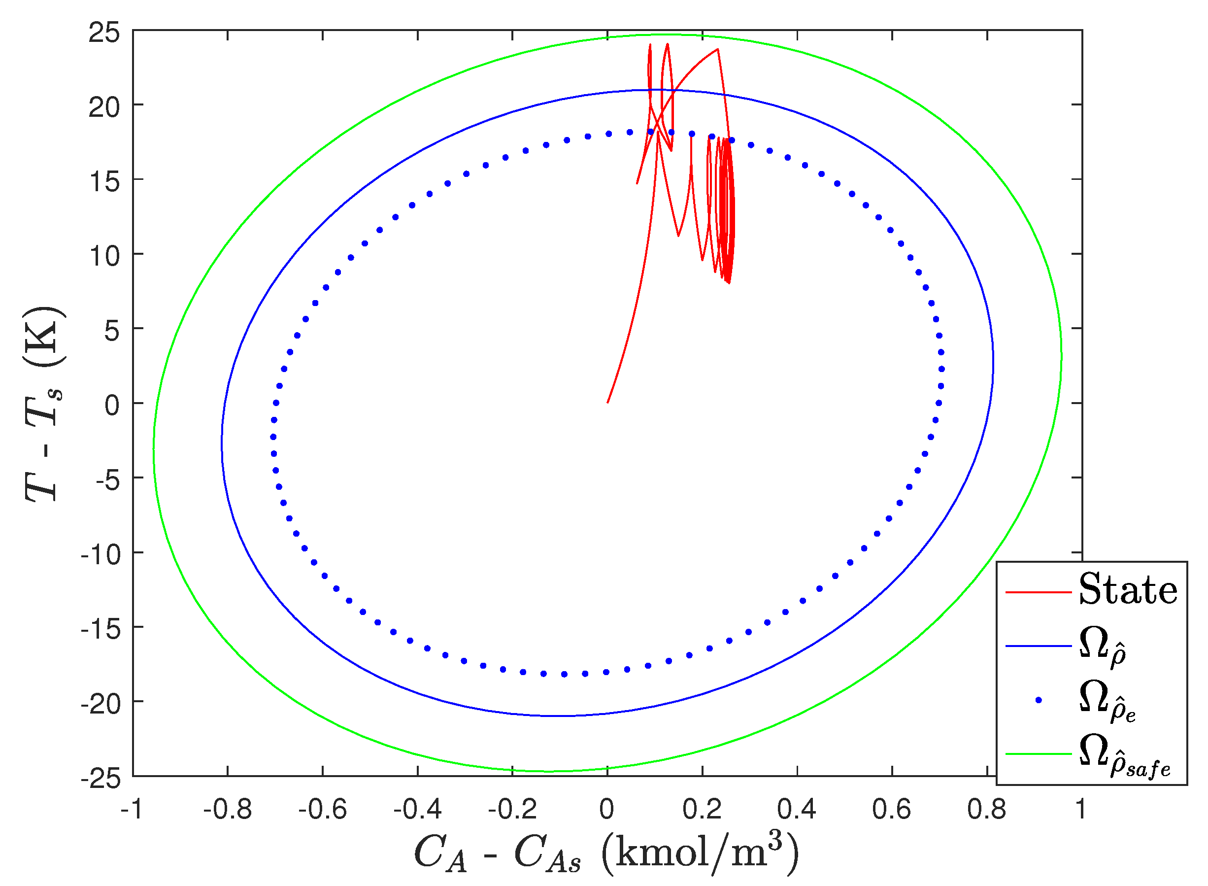In this case, with no change in the process model used by the EMPC or even in the control law (i.e., in contrast to the implementation strategy in Section 3.2.1, $h_{NL,1}$ is not employed when the closed-loop state exits ${\mathsf{\Omega }}_{\widehat{\rho }}$), the behavior in Figure 8 results. 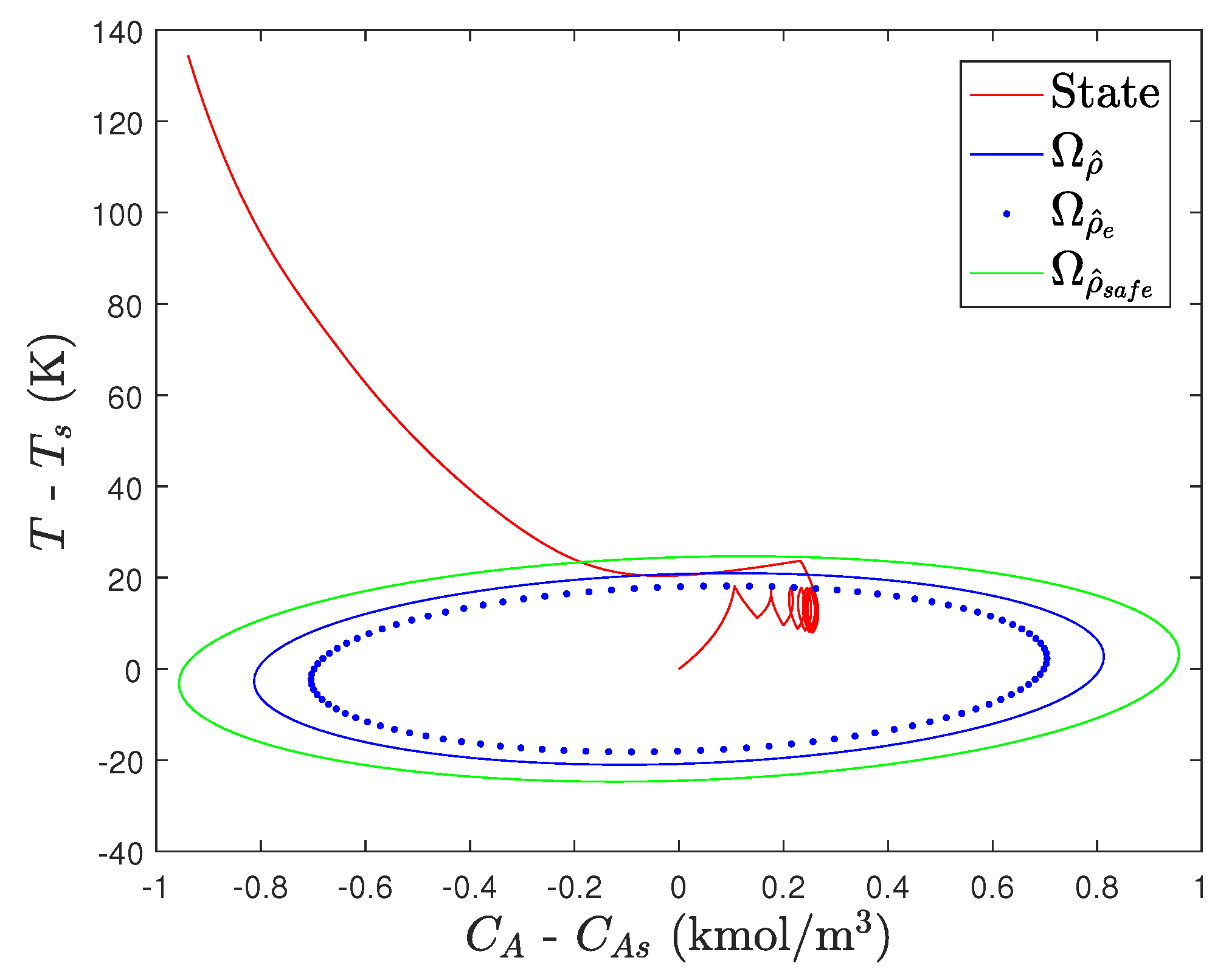Notably, the closed-loop state does not leave ${\mathsf{\Omega }}_{{\widehat{\rho }}_{safe}}$, and no infeasibility issues occurred. In contrast, if we begin to utilize $h_{NL,1}$ when the closed-loop state leaves ${\mathsf{\Omega }}_{\widehat{\rho }}$, the closed-loop state will eventually leave ${\mathsf{\Omega }}_{{\widehat{\rho }}_{safe}}$ (Figure 9). While we can obtain a new empirical model (in this case, we assume that the dynamics become fully known at 0.54 h and are accounted for completely to demonstrate the result) and can use that to update $h_{NL,1}$ to $h_{NL,2}$ (i.e., $h_{NL,1}$ but with modified saturation bounds to reflect design around the new steady-state of the system with $Q_{Added}=500$ K/h) before the closed-loop state leaves ${\mathsf{\Omega }}_{{\widehat{\rho }}_{safe}}$ as suggested in the implementation strategy in Section 3.2.1 (creating the profile shown in Figure 10 corresponding to 2 h of operation in which the closed-loop state is driven back to the origin under $h_{NL,2}$), the fact that the closed-loop state would not have left the stability region if the controller had not been adjusted illustrates the conservativeness of the approach. We note that Figure 10 does not complete the implementation strategy in Section 3.2.1 (which would involve the use of a new LEMPC after the closed-loop state reenters ${\mathsf{\Omega }}_{\widehat{\rho }}$ for this example) because that part of the implementation strategy will be demonstrated in the discussion for a slightly different LEMPC presented below.

Finally, we provide a result where the LEMPC computes a time-varying input policy due to the desire to enforce a constraint on the amount of reactant available in the feed over an hour (i.e., a material/feedstock constraint) as follows:

$$\frac{1}{1 \mathrm{h}} {\int }_{t=0 \mathrm{h}}^{t=1 \mathrm{h}}{u}_1(\tau )d\tau =0 \mathrm{kmol}/\mathrm{m}{}^3$$

(86)

This constraint is enforced via a soft constraint formulation by introducing slack variables $s_1$ and $s_2$ that are penalized in a modified objective function as follows:

$${\int }_{t_k}^{t_{k+N}}\left[-k_0{e}^{-\frac{E}{R_{g}T(\tau )}}{C}_A{(\tau )}^2\right]d\tau +100(s_1^2+s_2^2)$$

(87)

They are used in the following constraints:

$$\begin{array}{c}\hfill \sum _{i=0}^{k-1}(u_1^{*}(t_i|t_i))+\sum _{i=k}^{k+N_k}(u_1(t_i|t_k))-3.5\delta (100-\frac{t_k}{\Delta }-N)\le s_1\end{array}$$

(88)

$$\begin{array}{c}\hfill -\sum _{i=0}^{k-1}(u_1^{*}(t_i|t_i))-\sum _{i=k}^{k+N_k}(u_1(t_i|t_k))-3.5\delta (100-\frac{t_k}{\Delta }-N)\le s_2\end{array}$$

(89)

where $N_k=N$ and $\delta =1$ when $t_k<0.9$ h and where $\delta =0$ and $N_k$ is the number of sampling periods left in a 1 h operating period when $t_k\ge 0.9$ h. These constraints are developed based on Reference [12]. $u_1^{*}(t_i|t_i)$ signifies the value of $u_1$ applied to the process at a prior sampling time, and $u_1(t_i|t_k)$ reflects the value of $u_1$ predicted at the current sampling time $t_k$ to be applied for $t\in [t_i,t_{i+1})$, $i=k,\dots ,k+N_k$. The upper and lower bounds on $s_1$ and $s_2$ were set to $2\times {10}^{19}$ and $-2\times {10}^{19}$, respectively, to allow them to be effectively unbounded. The initial guesses of the slack variables were set to 0 at each sampling time.

When the LEMPC with the above modifications is applied to the process with $Q_{Added}=500$ K/h starting at 0.5 h, the closed-loop state again exits ${\mathsf{\Omega }}_{\widehat{\rho }}$ for some time after 0.5 h but reenters it and also does not exit ${\mathsf{\Omega }}_{{\widehat{\rho }}_{safe}}$, once again reflecting the conservatism from a closed-loop stability standpoint of a strategy that updates the process model whenever the closed-loop state leaves ${\mathsf{\Omega }}_{\widehat{\rho }}$. Furthermore, if $h_{NL,1}$ is utilized after it is detected that the closed-loop state leaves ${\mathsf{\Omega }}_{\widehat{\rho }}$ (the first sampling time at which this occurs is 0.51 h), then it exits ${\mathsf{\Omega }}_{{\widehat{\rho }}_{safe}}$ by 0.52 h, showing that the length of the sampling period or the size of ${\mathsf{\Omega }}_{\widehat{\rho }}$ with respect to ${\mathsf{\Omega }}_{{\widehat{\rho }}_{safe}}$ is not sufficiently small enough to impose model updates before closed-loop stability is jeopardized because measurements are only available every sampling time. If instead, however, $\widehat{\rho }$ is updated to be 1200 and ${\widehat{\rho }}_e$ is set to 900, then the closed-loop state remains in ${\mathsf{\Omega }}_{\widehat{\rho }}$ between 0.51 and 0.52 h. If at 0.52 h, we assume that the new dynamics (i.e., with $Q_{Added}=500$ K/h) become available and are used in designing $h_{NL,2}$ (used from 0.52 h until the first sampling time at which $x(t_k)\in {\mathsf{\Omega }}_{\widehat{\rho }}$ again) and that a second LEMPC designed based on the updated model is used after the closed-loop state has reentered ${\mathsf{\Omega }}_{\widehat{\rho }}$, the state-space trajectory in Figure 11 results.

4. Conclusions

This work developed a Lyapunov-based EMPC framework for handling unexpected considerations of different types. One of the types of considerations handled was end-user response to how a control law operates a process, providing a controller self-update capability through input rate of change constraints that allows even uncertain or imprecise information about the end-user response to be used in optimizing the controller formulation without loss of closed-loop stability or feasibility. The second type of consideration was the occurrence of anomalies, where conditions which would guarantee that the closed-loop state can be stabilized in the presence of an anomaly that changes the underlying process dynamics as long as a detection method identifies a new process model sufficiently quickly, were presented that uses the LEMPC stability properties in developing an anomaly detection mechanism. Chemical process examples were presented for both cases to demonstrate the proposed approach.

The work above provides insights into interpretability and verification considerations for EMPC from a theoretical perspective. However, these remain significant challenges for this control design. For example, there is no guarantee that adjusting a given constraint (e.g., adjusting the upper bound on an input rate of change constraint) will cause process behavior to appear interpretable to an end user before it approaches steady-state behavior, which may reduce the benefits of using EMPC. Furthermore, the results related to anomaly handling were demonstrated via process examples to be highly conservative. No methods were presented for practically ascertaining time (online) until an anomaly would result in the closed-loop state leaving a known region of state-space after detection to facilitate appropriate actions to be taken. Further work on these issues needs to be undertaken to develop practical EMPC designs with appropriate safety and interpretability properties with low time required to verify the designs before putting them into the field for different processes.